Stimulus-Related Neuroimaging in Task-Engaged Subjects Is Best Predicted by Concurrent Spiking

Abstract

The implicit goal of functional magnetic resonance imaging is to infer local neural activity. There is considerable debate, however, as to whether imaging correlates most linearly with local spiking or some local field potential (LFP) measurement. Through simultaneous neuroimaging (intrinsic-signal optical imaging) and electrode recordings from alert, task-engaged macaque monkeys, we showed previously that local electrophysiology correlates with only a specific stimulus-related imaging component. Here we show that this stimulus-related component—obtained by subtracting a substantial task-related component—is particularly linear with local spiking over a comprehensive range of response strengths. Matches to concurrent LFP measurements are, to varying degrees, poorer. As a control, we also tried matching the full imaging signal to local electrophysiology without subtracting task-related components. These control matches were consistently worse; they were, however, slightly better for gamma LFP than spiking, potentially resolving discrepancies between our findings and earlier reports favoring LFP.

Introduction

Techniques like blood oxygenation level-dependent (BOLD) functional magnetic resonance imaging (fMRI) are widely used since they hold the promise of inferring neural activity from imaging. The neural basis of imaging is still too poorly understood, however, to make such inferences unambiguously (Logothetis, 2008; Boynton, 2011; Buxton, 2013). An influential current belief is that imaging reliably measures local field potential (LFP) but not spiking. This derives from the proposition that the imaging response is driven by local metabolic demand, which, being dominated by the energetics of membrane voltage changes, is best captured by LFP (Logothetis and Wandell, 2004). A number of studies appear to support the superiority of LFP (Niessing et al., 2005; Viswanathan and Freeman, 2007; Goense and Logothetis, 2008; Bartolo et al., 2011), starting with the study by Logothetis et al. (2001), which showed that BOLD fMRI in the anesthetized monkey is modestly better predicted by concurrently recorded gamma LFP than spiking.

On the other hand, there is growing evidence that the primary local driver of neuroimaging is not metabolic demand per se, but rather synaptic glutamate release, possibly acting through astrocytes (Gurden et al., 2006; Attwell et al., 2010). In parallel, a number of studies point to a strong link between imaging and local spiking. The link was first proposed in studies that predicted human fMRI using monkey spiking (Heeger et al., 2000; Rees et al., 2000). More direct evidence comes from recent work showing that spikes evoked optogenetically in cortical pyramidal cells lead to local BOLD responses (Lee et al., 2010), even when synaptic transmission is pharmacologically blocked (Scott and Murphy, 2012).

The present study approaches this issue by asking whether imaging most linearly measures spiking or LFP. This study has two important methodological features that set it apart from earlier work. First, we matched local electrophysiology not to the full imaging but only to a specific stimulus-related component. This approach is based on our earlier finding that the imaging signal in alert, task-engaged macaques contains neurally distinct task- and stimulus-related components (Sirotin and Das, 2009). The task-related component is not predicted by local neural spiking or LFP and needs to be subtracted to reveal the match between stimulus-related imaging and local spiking (Cardoso et al., 2012). BOLD fMRI recordings from human subjects engaged in temporally structured tasks also report distinct task- and stimulus-related components (Jack et al., 2006; Donner et al., 2008). These results led to our starting premise that only stimulus-related imaging can be matched meaningfully to local spiking or LFP.

Next, we fit imaging to electrophysiology over a full range of response strengths to test the linearity of the fit as broadly as possible. With a few notable exceptions (Logothetis et al., 2001), LFP and spiking had earlier been compared with imaging at a single stimulus intensity, or using spontaneous activity (see Discussion), not allowing testing of linearity. Here, by contrast, we used a comprehensive dynamic range of stimulus intensities.

All data were obtained using our established technique of simultaneous electrode recordings and functional neuroimaging (intrinsic-signal optical imaging) from primary visual cortex (V1) of macaques performing visual tasks.

Materials and Methods

Simultaneous intrinsic-signal optical imaging and extracellular microelectrode recordings (Bonhoeffer and Grinvald, 1996; Shtoyerman et al., 2000; Sirotin and Das, 2009) were carried out in alert macaques engaged in passive fixation tasks (n = 65 sites; four hemispheres in two male monkeys). Data from a subset of 23 sites were used earlier for relating imaging to spiking (Cardoso et al., 2012). Methods here are essentially identical to those in the earlier article, with the addition of procedures specific to analyzing the LFP, and a modified procedure for fitting imaging to electrophysiology and assessing the goodness of fit. All experimental procedures were performed in accordance with the National Institutes of Health Guide for the Care and Use of Laboratory Animals and were approved by the Institutional Animal Care and Use Committees of Columbia University and the New York State Psychiatric Institute.

Behavior and stimuli.

Animals held fixation periodically for a juice reward, which was cued by the color of a fixation spot (fixation window, 1.0–3.5° in diameter; monitor distance, 133 cm; fixation duration, 3–4 s; trial duration, 10–20 s). Stimuli typically consisted of sine-wave gratings [contrasts, 0% (blank), 6.25%, 12.5%, 25%, 50%, and 100%; mean luminance = background luminance = 46 cd/m²; spatial frequency, 2 cycles/degree; drift speed, 4 degree/s; orientation optimized for the electrode recording site; diameter, 0.5–4° (fixed for a given experiment)]. Trials comprised single fixations, with stimulus presented during fixation. Stimuli were block randomized; that is, presented in blocks with each block containing a single full set of contrasts in random order. In the block, stimuli were repeated following errors (incorrect fixation) until the animal had a correct trial for each stimulus in a block. Some experiments included 3.125% contrast for finer resolution at low contrasts; others used a reduced set of contrasts to increase the number of trials per condition. Eye fixation and pupil diameter were recorded using an infrared eye tracker (Matsuda et al., 2000).

Surgery, recording chambers, and artificial dura.

After the monkeys were trained on visual fixation tasks, craniotomies were performed over their V1, and glass-windowed stainless steel recording chambers were implanted, under surgical anesthesia, using standard sterile procedures, to image an area of ∼10 mm of V1, covering visual eccentricities from ∼1 to 5°. The exposed dura was resected and replaced with a soft, clear silicone artificial dura. After the animals had recovered from surgery, their V1 was optically imaged, routinely, while they engaged in the fixation task. Recording chambers and artificial dura were fabricated in our laboratory using methods published previously (Arieli et al., 2002).

Hardware.

A Dalsa 1M30P camera (binned to 256 × 256 pixels, 7.5 or 15 frames/s) and a frame grabber (Optical PCI Bus Digital, Coreco Imaging) were used. Software was developed in our laboratory based on a previously described system (Kalatsky and Stryker, 2003). Illumination, high-intensity LEDs (Agilent Technologies and Purdy Electronics) with emission wavelength centered at 530 nm (green, equally absorbed by oxyhemoglobin and deoxyhemoglobin, and therefore a measure of local cortical tissue hemoglobin, i.e., blood volume). A macroscope of back-to-back camera lenses was focused on the cortical surface. Imaging, trial data (e.g., trial onset, stimulus onset, identity, and duration), and behavioral data (eye position, pupil size, timing of fixation breaks, fixation acquisitions, trial outcome) were acquired continuously. Data analyses were performed off-line using custom software in MATLAB [MathWorks (RRID:nlx_153890)].

Image preprocessing.

Before analysis, acquired images were (if necessary) motion corrected by aligning each frame to the first frame by shifting and rotating the images, using the blood vessels as a reference (Lucas and Kanade, 1981). Slow temporal drifts (>30 s) were removed with high-pass filtering, and cortical pulsations were removed with low-pass filtering using the Chronux (RRID:nif-0000-00082) MATLAB Toolbox function runline.m (typical heart rates were ∼2–3 Hz, much faster than the typical hemodynamic response frequencies of ∼<0.5 Hz).

Electrophysiology.

Electrode recordings were made simultaneously with optical imaging. Recording electrodes (FHC and Alpha Omega; typical impedances, ∼600–1000 kΩ) were advanced into the recording chamber through a silicone-covered hole in the external glass window, using a custom-made low-profile microdrive. Recording sites were mostly, but not exclusively, confined to upper layers. Measurements were recorded and amplified using a Plexon recording system (RRID:nif-0000-10382). The electrode recording was split into spiking (100 Hz to 8 kHz bandpass) and LFP (0.7–170 Hz) using the standard settings for the Plexon preamplifier. An additional analog two-pole 250 Hz high-pass filter was applied to the spiking channel by using the “noise filter” option in the Plexon on-line spike sorting. No attempt was made at isolating single units, and all measured spiking was multiunit activity (MUA) with “spikes” defined as each negative-going crossing of a threshold equal to ∼4× the rms of the baseline obtained while the animal looked at a gray screen. The neural measurements (MUA and LFP) were high-pass filtered to remove slow drifts (>30 s).

LFP spectral analysis.

The continuous time-varying LFP power spectrum for a full recording session was estimated for frequency bins 4–170 Hz using the multitaper method (Thomson, 1982) implemented in the Chronux MATLAB Toolbox. Different sets of parameters were used for frequency decompositions 4–30 Hz and 30–170 Hz. For the lower frequencies, we used 1000 ms windows displaced at 250 ms steps, a single taper, and a spectral concentration of ±1.0 Hz. For frequencies of 30–170 Hz, we used 250 ms windows displaced at 63 ms steps, three tapers, and a spectral concentration of ±8 Hz.

Preprocessing for fitting.

The core analysis of this study consisted of fitting measured imaging to each of a set of electrophysiological regressors, after separating into trials and grouping by contrast and averaging, as follows. The seven regressors comprised spiking (MUA), evoked LFP, evoked [LFP]², and four band-limited power (BLP) LFP measurements [4–12 Hz (“alpha + theta”), 12–30 Hz (“beta”), 30–90 Hz (“gamma”), and 110–170 Hz (“high gamma”)] obtained by averaging the time-varying induced LFP spectral power over the defined frequency bands. Regressors were downsampled to the imaging frame rate (7.5 or 15 samples/s); then they, along with imaging, were separated into trials aligned to trial onsets. Incorrect trials (i.e., those where the monkey either did not achieve fixation on time or broke fixation before the end) were rejected since the task-related response changes sharply for such trials (Sirotin et al., 2012). Trials containing artifacts—defined as transients larger than 35× the baseline SD—in any recorded response, imaging, or electrophysiology were discarded from the analysis along with the trials immediately following each contaminated trial. This process defined a common body of correct trials for all measurements. Each measurement was then converted to a z-score using the corresponding mean and SD for correct trials, and the trials were grouped by contrast and averaged. The responses at this point comprised the “full” responses.

Isolating stimulus-related responses.

Stimulus-related responses were isolated from each full response set (see above) by subtracting corresponding blank trial responses, aligned on trial onset. For imaging, according to our earlier model (Cardoso et al., 2012), this process removes a stereotyped task-related response that is locked to the trial period and is uniformly present in all correctly completed imaging responses, including blanks (Sirotin et al., 2012). In addition, for all response types, both electrophysiological and imaging, this step removes responses to incidental visual inputs at task periodicity such as those due to the animal looking around the room and back at the monitor on each trial (see the blank trial spiking response in Fig. 9A₁, which is low while the animal holds fixation and high while he is free to look around, including the burst of spikes as he starts looking around at the end of fixation; also see Sirotin and Das, 2009, their supplementary Fig. 1). What remains are the responses to controlled stimuli alone, which were then used for all subsequent calculations other than controls. For the controls (see Figs. 9, 10), we used the full responses.

Figure 9.

Full, non-blank-subtracted imaging is poorly fit by spiking and gamma LFP. A₁–B₃, Single case showing the full (i.e., non-blank subtracted) spiking (A₁) and LFP gamma (A₂), the corresponding predictions (B₁ and B₂), and the measured full imaging response (B₃; same example as in Fig. 2, following the same conventions). Note the prominent positive signal for the blank and low-contrast stimuli (compare with blank-subtracted measured imaging in Fig. 2B₃). Insets depict the optimal HRFs, with fits consistently poorer than for the corresponding blank-subtracted responses (compare Fig. 2B₁–B₃, insets). Note the large residuals (bottom panels), particularly for low-stimulus contrasts, which are comparable in amplitude to predicted signals.

Figure 10.

Overall, imaging is best fitted by spiking with blank-trial responses subtracted. A, Population distributions of fit R² values for the full (i.e., non-blank-trial-subtracted) responses. Data for fits to blank-trial-subtracted responses are repeated from Figure 4, for ease of comparison. Box plot conventions are as in Figures 4A and 8. B, Pairwise comparisons, experiment by experiment, for the control full-fit R² data illustrated in A. Scatter plots follow the same conventions as for the blank-subtracted data shown in Figure 4B. For control fits to the full signal without blank-trial subtraction, even though the statistical differences are weak, gamma band is comparable to and trends slightly higher than spiking (p values for the Wilcoxon signed rank test are depicted at the top center of each corresponding scatter plot).

Hemodynamic response function kernel fitting.

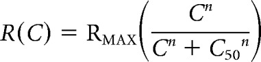
The hemodynamic response function (HRF) was modeled as a gamma variate function of the following form:

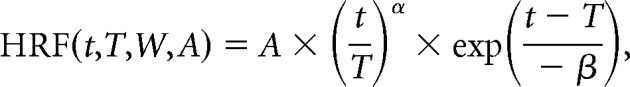where α = (T/W)² × 8.0 × log(2.0), β = W²/(T × 8.0 × log(2.0)), A is the amplitude, T is the time to peak, and W is the full-width at half-maximum (Madsen, 1992; Cohen et al., 1997; Sirotin and Das, 2009). This functional form allows for parametrically varying kernel amplitude, latency, and width. Since the fitted optimal HRFs typically extend to 10–15 s and peak at around 2–4 s (see Fig. 2), it is important to fit using a long enough sequence of measured responses to avoid end effects. We wanted to constrain the fit to be optimal for the full set of measured response strengths, and so the electrophysiological and imaging traces to be fitted against each other were constructed by explicitly concatenating responses of every stimulus contrast. Specifically, traces for fitting were generated as 50 concatenated blocks, where each block contained one set of average responses for each contrast with no repetition and each response aligned to trial onset. The sets in each block were randomly permuted with the same permutation for the neural and hemodynamic signals. The error function minimized in the fitting was constructed to give equal weight to the fractional error at each contrast: it consisted of the mean of the normalized squared error (SS_error/SS_total) calculated separately per contrast. The optimal HRF was obtained by minimizing this measure of error using a downhill simplex algorithm (fminsearch, MATLAB).

Figure 2.

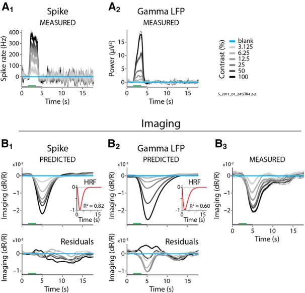
Spiking predicts imaging better than does gamma LFP. A₁, A₂, Single case example from Monkey S showing spiking (A₁) and gamma LFP (A₂) responses to gratings of six different contrasts. Conventions are as in Figure 1, with SEM (dashed lines) for N = 31 trials/contrast. The corresponding predictions made using, in each case, the optimal fitted HRF are shown in B₁ and B₂, respectively, while B₃ shows the measured imaging. Insets depict optimal HRFs (with typical time to peak of 2–4 s, and taking 10–15 s to decay back to baseline) and fit R² values, while bottom panels show the residuals indicating the differences between measured and predicted imaging. Note the larger residuals for LFP gamma compared with spikes.

Goodness of fit of predicted hemodynamics.

The R² used to quantify the goodness of fit was also defined to give equal weight to fractional errors at each contrast, complementing the error term minimized during fitting. Thus, R² was defined as the mean of the coefficients of determination (1 − SS_error/SS_total), calculated separately for each contrast. Note that this value of R² is more stringent and gives smaller values than the one used in the study by Cardoso et al. (2012). There, we simply calculated the overall coefficient of determination, where the numerator (SS_error) and denominator (SS_total) were summed over all contrasts.

Cross-validation of R².

To address overfitting, we performed a cross-validation procedure where the full set of trials in each experiment was divided randomly into “model” and “test” halves. The optimal HRF obtained for the model half of the trials was subsequently used to predict and obtain R² values for the test half. Since our stimuli were presented block randomized, we also selected subsets of trials blockwise (i.e., randomly selected entire blocks of trials for the model or test half). Note that for a typical experiment of 30 blocks, this gives 30!/(15! × 15!), or 1.5 × 10⁸ possible random splits. This random trial-splitting process was performed 200 times for each experiment, thus generating a distribution of R² values of which the median was defined as the estimated cross-validated R² for the experiment.

Linear regression of hemodynamic response against neural responses.

We linearly regressed the mean stimulus-related imaging, averaged within an appropriate response window (Fig. 1) and normalized to the maximum response, against the mean for each stimulus-related electrophysiological regressor (spiking or LFP) similarly normalized. The integration window for electrophysiology coincided approximately with the stimulus presentation period, while the integration window for imaging included the delay and duration of the blood volume response. Response linearity was quantified by the coefficient of determination (R² statistic in MATLAB regress.m, labeled “Regression R²” in this article).

Figure 1.

Stimulus-related imaging and electrophysiological responses to stimuli of different contrasts. A, Single case from Monkey S showing imaging, spiking, and LFP responses for each of four stimulus contrasts (of the six contrasts used). Each plot has the corresponding mean blank-trial (0% contrast) response subtracted, and is averaged over all correct trials (N = 30 per contrast). The imaging signal, proportional to local change in blood volume, is plotted as the fractional change in light reflected off the cortical surface (dR/R). The increased downward signal implies increased absorption of light and thus increased local blood volume. The LFP spectrogram (between 4 and 170 Hz) is shown separated into signals defined by the power lying within a set of frequency bins following a logarithmic progression [frequency bins are indicated to the right of the set of traces; the approximate standard labels (e.g., gamma and beta) are shown on the left; responses share a common vertical scale for signal power, shown on the right]. The evoked LFP and [LFP]² are shown at the bottom. Note the monotonically increasing imaging, spiking, and evoked LFP response amplitudes for increasing contrasts. Among the spectrally defined LFP traces, note the increasing gamma response power for increasing contrast. Beta LFP power shows a poorer response to visual stimulation. For frequencies between 4 and 12 Hz, increasing stimulus contrast leads to progressively more negative power responses (i.e., reduction in power below the baseline defined by the blank). Vertical spacing of the traces is arbitrary (chosen to optimize visualization). Ticks on the left and right of each trace indicate the 0 ordinate. Gray shading represents the window for calculating the LFP power spectrum (B₁, B₂) as well as response means used later to assess linear regressions (see Fig. 6); the spiking and all LFP responses share the same window, and the window for imaging is delayed and wider, reflecting its slower response dynamics. All responses are shown over one trial length, starting approximately at trial onset (3 s before stimulus onset); trial structure is indicated by bars below each column: gray, fixation; green, stimulus. A similar trial structure (albeit, sometimes with different timings) is used throughout the article. B₁, Population stimulus-related LFP power spectrum, separated by stimulus contrast, for Monkey S (left; N = 40 experiments) and Monkey T (right; N = 25). Spectra were computed separately for each experiment as the mean power within the response windows indicated in A, and then averaged across experiments. Solid lines show the spectra per stimulus contrast (color coded as shown alongside; identical color coding is used throughout the article), while thin dotted lines show the corresponding SEM limits. The response to the blank (blue curve) appears as a straight line at 0 power by definition, due to blank-trial subtraction. Note that the power spectrum for Monkey S has distinct positive peaks in the gamma (30–90 Hz) and beta (12–30 Hz) frequency ranges, and a negative peak in the alpha + theta (4–12 Hz) range. Vertical red dashed lines mark the frequency bounds defining BLP LFP measurements used in later analysis (see text). B₂, Stimulus-related LFP power spectrum for the example illustrated in A.

Results

We present data from 65 sites (four hemispheres, two monkeys), including 23 sites used earlier in the study by Cardoso et al. (2012). The animals' task and visual stimuli, and the experimental techniques used largely paralleled those used earlier (Cardoso et al., 2012). In brief, the animals fixated periodically for juice reward, cued by the color of a fixation spot (fixation periods of 3 or 4 s, at a trial period of 10–20 s but constant for a given experiment). The stimuli, presented passively during each fixation, comprised drifting sine wave gratings optimally oriented for the electrode recording site. The stimulus contrast typically doubled in steps starting from 3.125% or 6.25% up to 100%, allowing us to test the linearity between imaging and electrophysiology over a comprehensive dynamic range of stimulated responses. Stimuli were presented in blocks, with each block containing one complete set of stimulus contrasts, as well as a blank for blank-trial responses, in randomized order.

For neuroimaging, we used intrinsic-signal optical imaging (Bonhoeffer and Grinvald, 1996; Shtoyerman et al., 2000). This technique estimates changes in local cortical blood volume and oxygenation by imaging the exposed brain surface at wavelengths absorbed by hemoglobin. Even though the underlying technologies are distinct, optical imaging and fMRI are closely related in the information they provide. Simultaneous optical and fMRI BOLD studies in rat cortex show that the hemodynamic measurements obtained using optical imaging reliably predict the concurrent BOLD response and vice versa (Kennerley et al., 2005, 2009; Martindale et al., 2008). Here we imaged at a wavelength selective for total hemoglobin (i.e., blood volume; Devor et al., 2003; Nemoto et al., 2004; Sheth et al., 2004; Sirotin et al., 2009). The optical response at this wavelength matches fMRI measurements of local cerebral blood volume (Fukuda et al., 2006). Further, the impulse response to a brief sensory stimulus is monophasic and is reliably represented as a single gamma-variate HRF (Sirotin et al., 2009), making the imaged response easy to interpret and to model mathematically. The concurrent electrode recording was processed for both high frequencies [i.e., spiking (250 Hz to 8 kHz), specifically MUA] and low frequencies [i.e., the LFP (0.7–170 Hz)].

The LFP was further processed to obtain a number of complementary measures of both the induced and the evoked response (Galambos, 1992; Tallon-Baudry and Bertrand, 1999). Induced responses comprise stimulus-linked changes in signal fluctuations that are at best loosely phase locked to stimulus timing and thus cancel out on averaging the LFP. To measure induced LFP, we first calculated the continuous, time-varying LFP power spectrum (see Materials and Methods). The spectrally separated components were combined to define a set of BLP LFP measurements (see next section), which were then separated by trial and contrast. For evoked responses phase locked to the stimulus, we considered the raw LFP and [LFP]² (i.e., the evoked power). Unlike the power spectrum, these signals preserve phase information. Thus, the mean LFP, averaged across trials, accentuates response features such as stimulus-onset transients (Fig. 1). On the other hand, response fluctuations not similarly phase locked—such as the prominent gamma-band oscillation that typically follows stimulus presentation—are averaged away, even though they contribute substantially to the power spectrum of the induced LFP. The evoked and induced LFP thus carry complementary information.

We then isolated the stimulus-related parts of the imaging, spiking, and LFP measurements, by subtracting the corresponding blank-trial responses (see Materials and Methods), to compare how linearly the stimulus-related imaging, per se, correlates with stimulus-related LFP as versus spiking. This crucial feature of the current analysis is based on earlier findings from studies using monkeys in our laboratory (Sirotin and Das, 2009), as well as from human BOLD fMRI data from at least two other laboratories (Jack et al., 2006; Donner et al., 2008; Pestilli et al., 2011), that imaging measurements from visual cortex of subjects performing visual tasks contain distinct task- and stimulus-related components. With concurrent imaging and electrode recordings from monkey V1, we showed that the task-related component is not correlated with local spiking or LFP. It thus needs to be removed from the overall measured imaging—for example, by subtracting blank-trial responses—to avoid substantial errors when relating imaging to local electrophysiology (Sirotin and Das, 2009; Cardoso et al., 2012). The stimulus-related imaging component thus isolated, however, is strikingly well correlated to stimulus-related local spiking (Cardoso et al., 2012). The core of the current study consists of asking how well it correlates with various stimulus-related LFP measures. For brevity, we will drop the prefix stimulus-related and refer to responses simply as imaging, spiking, or LFP.

Contrast response varies across different measurements of cortical activity

A representative set of responses (Fig. 1A) demonstrates the distinct behaviors of imaging and the various electrophysiological measurements across stimulus contrasts. Comparing among these responses also gives us an initial intuition as to whether spiking or one of the LFP measurements is likely to best match imaging over the full range of response strengths.

Imaging and spiking each have their expected, largely stereotyped responses, with amplitudes that increase uniformly with stimulus contrast. Both response profiles are also essentially monophasic: the imaging response consists of a delayed, downward pulse of increased light absorption by cortex, reflecting increased local blood volume, that returns slowly to baseline (Sirotin et al., 2009), while the spiking rises from and returns to baseline over an interval that crisply reflects stimulus duration.

The induced LFP spectral signals on the other hand—analyzed, initially, into a regular progression of spectral bands to avoid assumptions regarding optimal frequency separation—show responses that differ sharply by frequency. At higher frequencies (>12 Hz), the LFP response, like spiking, increases with stimulus contrast. Below 12 Hz, however, increasing stimulus contrast leads to progressively greater suppression of LFP power below the blank-trial (i.e., 0% contrast) baseline. Spectral analysis of the stimulus-induced LFP response per contrast (lying within a stimulus-defined window; Fig. 1A, gray stripes) shows that these distinct response patterns cluster approximately by established LFP frequency bands (Fig. 1B₁, population average power spectra, B₂, power spectrum of the single case in A). The robust stimulus-induced suppression, growing stronger with stimulus contrast, is seen in a frequency band (4–12 Hz) that combines alpha and theta bands. The positive stimulus-induced responses, on the other hand, separate into two distinct bands comprising 12–30 Hz and 30–90 Hz, coinciding approximately with beta and gamma bands, respectively (Fig. 1B₁, left). We used these frequency bands to define BLP LFP measurements to match with imaging, for both animals even though the band separation in Monkey S was crisper than in Monkey T (Fig. 1B₁, left and right, respectively).

A comparison of these BLP LFP responses with spiking suggests, however, that spiking may match imaging better than any response, for varying reasons. LFP responses in the 30–90 Hz range (i.e., gamma range) are monophasic, crisp, and stereotyped like spiking (for example, Fig. 1A, 58.1–71.4 Hz band), but their amplitude progression is notably different. While spiking, like imaging, grows in uniform steps with stimulus contrast, starting at the lowest contrast, the gamma LFP response is low at low contrasts and rises sharply at high contrasts. This suggests that imaging may be less linear with gamma LFP than with spiking. Responses at the two lower frequency ranges (4–12 Hz and 12–30 Hz) grow steadily stronger with stimulus contrast albeit in different directions. However, the response time courses are rather noisy and exhibit different profiles across contrasts, suggesting low reliability as a predictor of imaging response shape.

Evoked LFP and [LFP]² responses are different from spiking or induced LFP measurements in any spectral band. Though their responses grow steadily stronger with stimulus contrast, as with imaging or spiking, the response profiles are dominated by sharp onsets and offsets with otherwise weak signals relative to background over the stimulus duration. This response profile suggests that they—particularly, the biphasic evoked LFP—may be poorer than spiking in predicting the monophasic imaging response shape. Despite this, we felt that it was important to include them in our analysis, for completeness, since evoked EEG (e.g., the visually evoked potential) is still commonly used as a diagnostic and investigational tool for human studies (Creel, 2012).

Based on the distinct response patterns seen in Figure 1, we defined seven electrophysiological regressors to compare separately with imaging. The regressors are spiking (MUA), evoked LFP and [LFP]², and three BLP LFP measures consisting of the spectral power in the 4–12 Hz (alpha + theta), 12–30 Hz (beta), and 30–90 Hz (gamma) bands. In addition, we defined a fourth BLP LFP measure comprising induced power in the 110–170 Hz (high-gamma) band (Fig. 1), even though there is no peak in response power in this frequency range, the mean signal is an order of magnitude weaker than gamma LFP, and there are concerns that it may largely just reflect local spiking (Ray and Maunsell, 2011; Zanos et al., 2011). We did so for completeness, as this frequency range has been used both in animal LFP (Goense and Logothetis, 2008) and human electrocorticography studies (Mukamel et al., 2005; Canolty et al., 2006), including comparisons with fMRI (Mukamel et al., 2005; Goense and Logothetis, 2008). The frequency range 90–110 Hz was discarded in our analysis to avoid an occasional 100 Hz pickup from our display monitor.

Imaging is best predicted by spiking

To compare how well the regressors defined above predict imaging, we fitted each of them in turn using gamma-variate HRF kernels (Madsen, 1992; Cohen, 1997; Sirotin and Das, 2009). In each case, optimal HRFs and predictions were obtained, as usual, by parametrically varying kernel parameters to minimize the normalized squared error between predicted and measured imaging (see Materials and Methods). Each fit was performed across all stimulus contrasts simultaneously to obtain fits that were optimal over the full response dynamic range. The goodness of fit, defined as R², was quantified as the mean of the coefficients of determination between measured and optimal predicted responses: (1 − sum squared error/sum squared measured response) calculated separately at each contrast. It was also the complement of the quantity minimized during fitting (see Materials and Methods).

A comparison of the resultant fits showed both that spiking predicted imaging reliably, and that it was better than any LFP measure. This can be illustrated by comparing the fits to spiking with those to gamma LFP (30–90 Hz) for one specific example dataset (Fig. 2). The imaging responses predicted by spiking (Fig. 2A₁,B₁), using the optimal fitted HRF (Fig. 2B₁, inset) match measured imaging responses (Fig. 2B₃) well, contrast by contrast. This good match leads to modest residual errors (Fig. 2B₁, bottom) and a robust R² = 0.82. For gamma LFP, on the other hand (Fig. 2A₂,B₂), the match is distinctly poorer (R² = 0.60) with larger residuals (Fig. 2B₂, bottom) that vary with stimulus contrast. Similar comparisons also show spiking to be consistently superior—albeit to varying degrees—to the remaining five electrophysiological predictors for the same dataset (Fig. 3). The particularly good match of imaging to spiking is also evident in a grand comparison of R² values across the population of experiments (Fig. 4A). High-gamma (110–170 Hz) and gamma LFP also fit imaging reasonably well, but significantly less so than spiking, as seen quantitatively through pairwise comparisons of R² values per experiment (Fig. 4B). The other LFP measurements, alpha + theta (4–12 Hz), beta (12–30 Hz), and the evoked LFP responses, fit imaging much worse (Figs. 3, 4). Note, parenthetically, that these results were obtained with no attempt on our part to optimize stimulus size (Henrie and Shapley, 2005). Our stimuli, with diameters ranging from 0.5° to 4°, likely induce varying degrees of nonlinear surround effects. These effects are of opposite sign (i.e., are suppressive for spiking; Cavanaugh et al., 2002) and facilitatory for gamma LFP (Gieselmann and Thiele, 2008). The observation that imaging correlates better with spiking than with any LFP measure despite the variable degree of surround interactions highlights the reliability of the match to spiking.

Figure 3.

LFP responses and corresponding predictions for the same experiment as in Figure 2, but for the BLP LFP alpha + theta, beta, and high-gamma bands, and for evoked LFP and evoked [LFP]² values. Conventions are as in Figure 2. A₁–A₅, Measured LFP responses. B₁–B₅, Corresponding predictions (top), optimally fitted HRF and fit R² values (inset), and residuals (bottom). B₆, Measured imaging (repeated here from Fig. 2B₃ to aid comparison).

Figure 4.

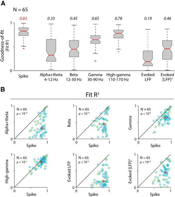
Population comparisons of goodness of fit (R²) show that imaging is consistently better predicted by spikes than by any LFP measure. A, Box plots showing population distributions of R² (N = 65 experiments, two monkeys) for fitting imaging to spikes and to each LFP measure in turn, as labeled. Median R² values are represented by horizontal red bars (values are also listed above). The bottom and top edges of each box represent the 25th and 75th percentiles, respectively. Whiskers extend to the most extreme data point not considered to be an outlier. Outliers (red crosses) are data points that exceed 1.5 times the first to third quartile distance either below or above. Nonoverlapping notches indicate that medians differ at the 5% level (a conservative estimate based on the assumption that measurements were independently acquired). Note that the notches for spiking only overlap with those for high-gamma LFP, indicating the superiority of spiking over other LFP measures even with this conservative assumption. Since our signals were acquired simultaneously (i.e., not independently), we were able to perform pairwise comparisons, experiment by experiment. B, Pairwise comparisons of R² values for each LFP regressor, as labeled (y-axes), against corresponding spike-fitted R² values (x-axes). Note that the spike-fitted R² value is consistently higher than R² values for fits to any LFP measure tested, including high-gamma band. Diagonals represent the equality line, and red crosses indicate medians; p values (Wilcoxon signed rank test, depicted at the top left of each scatter plot) estimate the probability that the pair of datasets comes from the same distribution. Data are shown color coded by monkey: blue for Monkey S (N = 40 experiments); and green for Monkey T (N = 25 experiments).

For the above results, both HRF fits and subsequent tests (i.e., calculation of R²) used the full set of trials for each experiment. This was done to accommodate some experiments with limited numbers of trials, but it raises the concern of overfitting. To address this, we carried out a cross-validation procedure where trials in each experiment were split randomly 200 times into model and test halves with optimal fits obtained for the model then used to get predictions and R² values for the test (see Materials and Methods). The cross-validated R² for each experiment—defined as the median of the test R² distribution—largely reproduced the overall pattern of R² across experiments and across regressors seen in Figure 4. These results confirmed the superiority of spiking over all LFP measures and provided confidence that overfitting was not a serious issue in our analysis. This is illustrated for spiking and gamma LFP [Fig. 5A,B (with Fig. 5A showing the same single case as in Fig. 2)] and tabulated for the other regressors (Fig. 5C).

Figure 5.

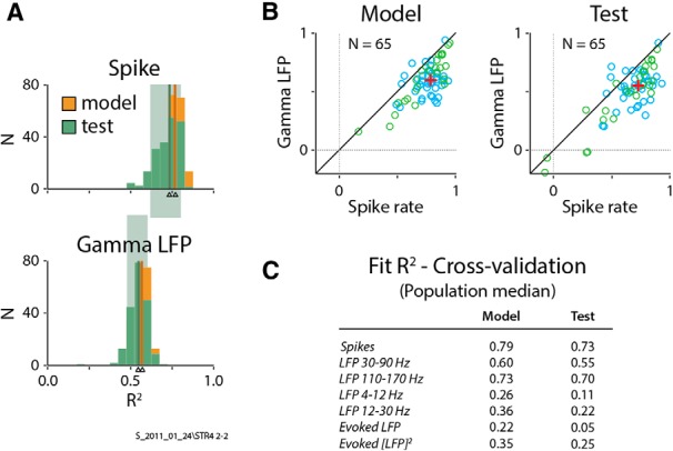
Cross-validation confirms spiking as the best predictor of imaging. A, Histograms of R² values for individual cross-validation runs from the same experiment as in Figure 2 (N = 200 runs; see text for details). Both model and test R² sets are shown, color coded as indicated, for imaging versus spikes (top) and imaging versus gamma LFP (bottom). Thin color-coded vertical bars (indicated by arrowheads) represent median R² values for each set, while background rectangles indicate the central 80% of the test sets. Note the largely higher R² values for spiking over gamma LFP, including higher median values as well as the lack of overlap of their respective central 80%. Additionally, the substantial overlap of each model and test R² histogram indicates that overfitting was not a serious issue in our analysis. B, Pairwise comparisons, experiment by experiment, of cross-validated R² for gamma LFP versus spikes, plotting medians calculated as in A for each experiment. Conventions are as in Figure 4B, with crosses indicating population medians over all experiments (N = 65). Note the similarity of model and test with each other and with the gamma LFP versus spikes plot in Figure 4B, albeit shifted to slightly lower values, as expected due to the reduced number of trials. This overall similarity and the consistent superiority of spiking over gamma LFP, points to the robustness of our main finding. C, Summary of cross-validation results. Table shows population median values (model and test), equivalent to the red crosses in B but for all regressors. Note the good match with R² values calculated using full sets of trials (Fig. 4A), albeit with slightly smaller values, as expected due to the reduced number of trials.

The basis for a good fit: amplitude linearity combined with matched response shape

What accounts for the particularly good match of spiking to imaging and its superiority over all other predictors? Understanding this issue would help to define a framework for comparing our analysis and findings with earlier results. We reasoned that the answer lies in our performing the fit over the full dynamic range of response strengths. Thus, for a good fit, not only do predicted and measured responses need to match each other in shape, they also need to match in strength (i.e., be linear with each other) over the full dynamic range.

We thus re-examined each fit in terms of these two factors, linearity and shape similarity. To quantify linearity, we regressed imaging against each regressor in turn, with response strengths being defined as averages within appropriate integration windows (as specified in Fig. 1A). To quantify response shape similarity independent of response strength, we correlated the predicted versus the measured imaging responses using Pearson's r, a measure invariant to scale and position shifts. Analysis on the basis of these two factors showed both that spiking was more linear with imaging and that it gave more accurate shape predictions than did any LFP measure.

The reason for the consistently high linearity of spiking can be easily appreciated by first plotting the spiking, imaging, and gamma LFP response strengths as functions of stimulus contrast (Fig. 6A) for the same dataset as in Figure 2. Spikes and imaging shared remarkably similar contrast responses (Fig. 6A₁,A₂). Both showed a compressive nonlinearity with stimulus contrast, and they were well fitted by hyperbolic sigmoids with similar parameters, consistent with our earlier work (Cardoso et al., 2012). In sharp distinction, gamma LFP power increased relatively monotonically with contrast (Fig. 6A₃), with much less saturation at high contrasts, which again is consistent with earlier findings (Henrie and Shapley, 2005) and with the qualitative observations following Figure 1A. Consequently, while imaging was homogeneously linear when regressed against spiking (Fig. 6B₁), with unity slope, a zero intercept and high regression R², it showed a distinct compressive nonlinearity when plotted against gamma LFP (Fig. 6B₂). This nonlinearity makes linear regression not the best model for the gamma LFP plot; the calculated regression line had a shallower slope, a non-zero intercept, and lower R² values. Imaging is usefully linear with gamma LFP at higher contrasts (e.g., at >12% contrast; Fig. 6B₂, four top data points). However, this linearity needs to be interpreted with caution since the corresponding regression line would intercept the imaging axis (y-axis) at approximately half the maximum value. Thus, half the maximum imaging amplitude, according to the linear regression, would correspond to zero gamma power, a conclusion that is inconsistent with the measured results. Similar patterns were seen across the population, with imaging being consistently linear with spiking (Fig. 6C₁) while being consistently compressively nonlinear with gamma LFP (Fig. 6C₂). It is important to emphasize that this difference in pattern is not an artifact of, say, higher noise in gamma LFP. If anything, gamma LFP has lower trial-by-trial variability than spiking, as can be appreciated by comparing SEM error bars (e.g., compare errors Figs. 2A₁ vs A₂, or 6A₁ vs A₃).

Figure 6.

Spiking is more linear with imaging and predicts its shape better than does gamma LFP. A₁–A₃, Plots of spiking (A₁), imaging (A₂), and gamma LFP (A₃) as functions of stimulus contrast, for the same experiment as in Figure 2. Data points (circles) indicate normalized mean responses ± SEM (vertical lines; N = 31 trials/contrast) here and in B₁ and B₂. Red traces depict the optimally fitted hyperbolic sigmoid response function R(C) of contrast C, of the following form:

(Albrecht and Hamilton, 1982; Cardoso et al., 2012). Note the similarity of the contrast response for imaging and spikes, captured by the similarity of their fit parameters, compared with gamma LFP [the fitted R_MAX values, n, and C₅₀ (the semisaturation constant) are listed in each panel with the discrepant values for gamma LFP highlighted in red]. B₁, B₂, Same data, with imaging plotted against spiking (B₁) and gamma LFP (B₂). Linear regression R² values and equations are indicated in each panel. C₁, C₂, Population scatter plots for imaging versus spiking (C₁) and gamma LFP (C₂), combining normalized responses as in B₁ and B₂, respectively, across all experiments [N = 261 points for Monkey S (blue circles); N = 109 points for Monkey T (green circles)]. Gray lines show linear regressions for each individual experiment (N = 65). D₁, D₂, Shape comparison between measured imaging responses and those predicted from spikes (D₁) and gamma LFP (D₂) for the same experiment as in A. Traces are shown with mean subtracted and normalized by SD to make their shapes easier to compare. Spike predictions matched the measured imaging shape better than gamma LFP predictions, as quantified by the mean Pearson's r values (increasing order of stimulus contrast: r = 0.88, 0.93, 0.94, 0.98, 0.97, 0.94 for spikes vs imaging; r = 0.52, 0.71, 0.88, 0.95, 0.96, 0.97 for gamma LFP vs imaging), giving mean values of 0.94 and. 0.83, respectively, for spiking and gamma LFP.

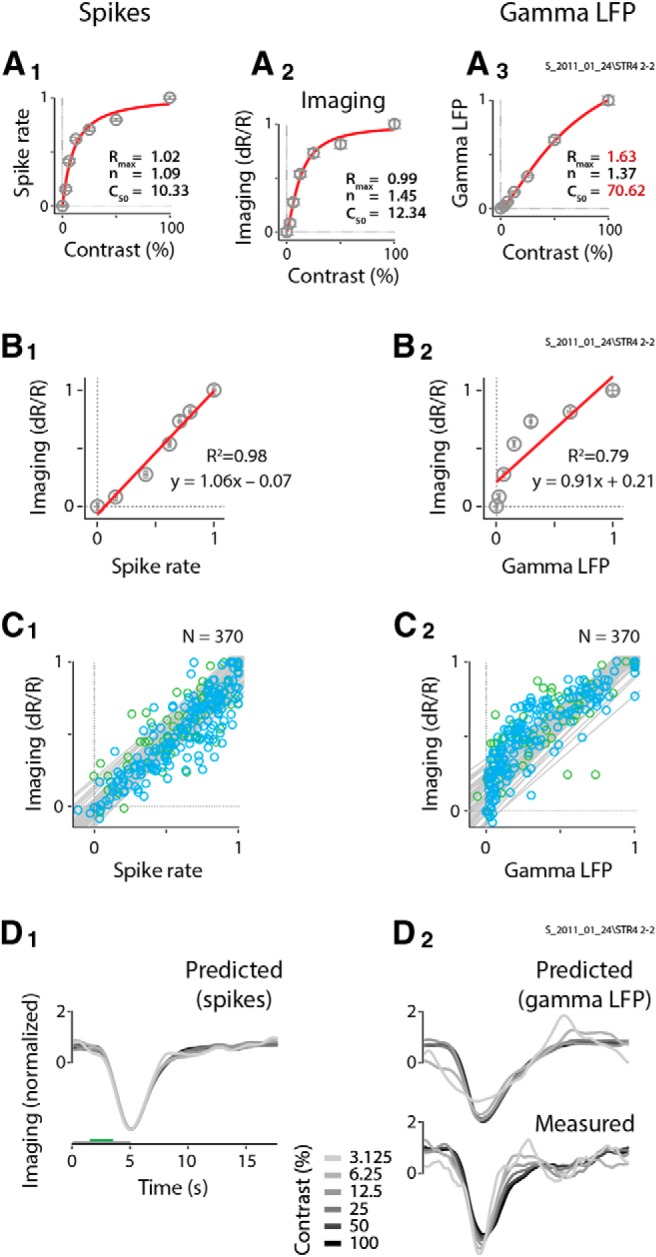
A comparison of response shapes showed that the predictions made using spiking (Fig. 6D₁), while not capturing the finer features of the measured imaging time course (Fig. 6D₂, bottom), correlate well with it overall, with high Pearson's r values at each contrast. This good match leads to a high shape match for the experiment, which we quantify using the mean Pearson's r value. Similarly good matches in response shape were seen across the population, giving mean correlation values per experiment that were also tightly clustered close to 1 (see Fig. 8B). The shapes predicted from gamma LFP (Fig. 6D₂) were slightly, but significantly, less correlated with imaging compared with predictions made from spiking. This relative shape mismatch was also observed over the population, as quantified through pairwise comparisons with the correlation for spiking (see Fig. 8B, caption).

Figure 8.

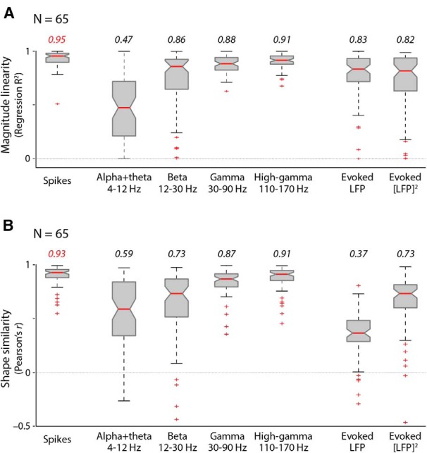
Spiking is more linear with imaging and predicts its shape better than any LFP response type, over the full population of experiments. A, Comparison of linearity. Box plots show population regression R² values for imaging versus each electrophysiological measurement indicated (N = 65 experiments). Conventions for medians, quartiles, and outliers are as in Figure 4A. In addition, pairwise comparisons of regression R² using spikes (first column) versus all LFP measures in turn, experiment by experiment, show that spiking yields significantly higher values (Wilcoxon signed rank test with p values for spike vs LFP measures: alpha + theta band, 10⁻¹¹; beta band, 10⁻⁷; gamma band, 10⁻⁴; high-gamma band, 0.04; evoked LFP, 10⁻⁷; and evoked [LFP]², 10⁻⁸). B, Imaging predicted from spikes shows the best shape similarity (mean Pearson's r across contrasts) with the measured imaging signal. Box plots of the shape similarity were measured over the population, with conventions as before. Note the similar trend for shape similarity and regression R² values across the different response types, with the exception of evoked LFP, which has a reasonable linearity with imaging but predicts an imaging shape quite dissimilar to the one measured (compare the fourth column of Fig. 7 for a single case example). Pairwise comparisons of shape similarity measures over the population again show spiking to be superior. The corresponding Wilcoxon signed rank test p values for spiking versus the following: alpha + theta band, 10⁻¹¹; beta band, 10⁻⁹; gamma band, 10⁻⁵; high-gamma band, 10⁻³; evoked LFP, 10⁻¹¹; and evoked [LFP]², 10⁻¹⁰.

The fits of imaging to the other five predictors were all worse than fits to spiking, for both linearity and shape similarity. These analyses reflect the comparisons with imaging assessed qualitatively in Figure 1A. Because of nonmonotonic responses, linear regression was often a very poor model for relating imaging to an LFP regressor (Fig. 7A₁); however, it is instructive to perform the regression analysis to get a measure of the degree of variability for the different response types. In regression analysis, alpha + theta (4–12 Hz) was worst, with both positive and negative slopes across the population of experiments (Fig. 7A₁,B₁) and low regression R² values (Fig. 8A). Beta band (12–30 Hz) had good regression R² values for individual cases (Fig. 7A₂) and overall for the population (Fig. 8A), though with some variability across experiments (Figs. 7B₂, 8A). The high-gamma band came closest to spiking (Fig. 7A₃), though its regression R² values were still lower compared with spikes (Fig. 8A). Note that regression fits to beta band and evoked [LFP]² values were very different in the two animals, with positive versus negative slopes, suggesting that these two LFP measurements are likely individual, specific, and unreliable compared with gamma LFP and high-gamma band values, and thus are particularly unreliable as predictors of imaging. In comparing predicted shapes, evoked LFP is noteworthy: the biphasic profile of this LFP response results in a similarly biphasic optimal prediction that is strikingly poorly matched in shape to measured imaging (Figs. 7C₄, 8B), verifying the shape mismatch predicted qualitatively in Figure 1A. This leads to an expected poor overall R² for the fit (Fig. 4), even though evoked LFP is reasonably linear with imaging in response strength (Figs. 7A₄,B₄, 8A). Of the other predictors, alpha + theta band, and to a lesser extent beta band, predicted shapes that were particularly noisy and variable (Figs. 7C₁,C₂, 8B), verifying the assessment from Figure 1A, while high-gamma band predicted reliable shapes comparable to those of spiking (Figs. 7C₃, 8B).

Figure 7.

Regressions of imaging versus LFP responses, and comparisons of predicted versus measured response shapes. Analyses and conventions are as in Figure 6, but for the LFP bands alpha + theta, beta, high gamma; evoked LFP; and evoked [LFP]². A₁–A₅, Linear regressions for imaging versus the electrophysological responses, as labeled. Data points show the normalized mean response strengths for the same experiment as in Figure 6, calculated as in Figure 6, B₁ and B₂. B₁–B₅, Population scatter plots for imaging versus electrophysiological response strengths, as in Figure 6C, with regressions for individual experiments shown as gray lines. C₁–C₅, Shape comparison between measured and predicted imaging for the same experiment as in A₁ and A₂. Mean Pearson's r correlation values across contrasts, used to quantify shape similarity between measured and predicted imaging, are as follows: alpha + theta bands, 0.47; beta band, 0.73; high-gamma band, 0.93; evoked LFP, 0.32; evoked [LFP]², 0.84.

Control: comparing with fits to the full signal

Our results so far show that the stimulus-related component of imaging is best matched by spiking. As a control, we wanted to confirm that this match was better than that of the full imaging response (i.e., without removing the task-related component) to any local electrophysiological measurement, spiking or LFP. To test this, we defined a new set of seven electrophysiological predictors in a manner identical to the predictors for stimulus-related imaging, though this time without subtracting blank-trial responses. We then fitted the full imaging response to each of these predictors as before to obtain a new set of optimal HRFs, predictions, and goodness of fit (R²) values.

The control fits for the full responses were consistently and substantially worse than the fit of stimulus-related imaging to spiking. This result is illustrated in Figure 9 for fits to spiking and gamma band, for the same experiment as in Figure 2. The new fits leave large residuals leading to strikingly poor R² values (compare Fig. 2). Note that the residuals are largest for the blank trial (Fig. 9B₁,B₂, bottom panels), which is consistent with our starting premise that the full imaging response contains a stereotyped task-related component unexplained by local neural activity (see also Cardoso et al., 2012, their Fig. 1). Similarly poor fits to the full response were seen across the population, and for all predictors, spiking, and LFPs (compare Fig. 10A, which repeats the earlier fits to stimulus-related responses).

Notably, however, the distribution of R² values for these control fits across spiking and the different LFP bands bears a striking resemblance to earlier published correlations (see Goense and Logothetis, 2008, their Fig. 4), which were also performed without subtracting task-related imaging. The magnitudes of our control R² values—all much worse than our fit of stimulus-related imaging to spiking—are approximately comparable to the earlier published R² values. Moreover, our control fits to gamma LFP, while being close in value to the corresponding control fits to spiking, trend slightly higher over the population (Fig. 10B), like the earlier reported advantage of LFP over spiking (Logothetis et al., 2001; Goense and Logothetis, 2008). Finally, our distribution of control R² over BLP LFP bands (Fig. 10A), starting low for low frequencies (alpha + theta, 4–12 Hz), peaking broadly around beta band (12–30 Hz) and gamma band (30–90 Hz), and then dropping again at higher frequencies (high-gamma band, 110–170 Hz), resemble earlier reported correlations peaking broadly around “nMod” (defined as 20–60 Hz) and gamma band (65–100 Hz), while dropping to lower values for both lower and higher LFP frequencies (Goense and Logothetis, 2008). This suggests that the earlier studies may have obtained the patterns they did (i.e., poor R² values overall, but better for gamma LFP than for spiking) as a result of not subtracting task-related imaging components.

Discussion

Here we asked whether V1 neuroimaging in alert, task-engaged monkeys correlates most linearly with local spiking or with some LFP measure. After removing the task-related component, we showed that imaging matches spiking best, both in linearity of response strengths and shape of predicted responses. All LFP predictors gave poorer matches, in shape, linearity, or both (Figs. 4, 8). The high-gamma band (110–170 Hz) was the best LFP predictor, but that may reflect its close link to local spiking, whether due to spectral leakage (Zanos et al., 2011) or common physiological processes (Ray and Maunsell, 2011). Control fits to the full imaging without removing the task-related component were uniformly inferior. Notably, the fits to spiking and gamma LFP in this control set were approximately comparable to each other, with gamma LFP trending to be slightly stronger (Fig. 10).

Two important features distinguish this study and largely set it apart from others that have compared local spiking to LFP as predictors of neuroimaging (Mathiesen et al., 1998; Logothetis et al., 2001; Niessing et al., 2005; Viswanathan and Freeman, 2007; Goense and Logothetis, 2008; Murayama et al., 2010; Kahn et al., 2013).

The first feature is our starting premise that imaging in alert task-engaged subjects contains a neurally distinct task-related component that needs to be removed before matching to local electrophysiology (Sirotin and Das, 2009; Cardoso et al., 2012). The premise is corroborated here by our control measurements (Figs. 9, 10). Notably, at least two groups have reported a task-related component in human fMRI; as in our findings, this component needed to be subtracted before relating imaging to stimulation (Jack et al., 2006; Donner et al., 2008; Pestilli et al., 2011). The human fMRI studies did not, however, include the electrode recordings that allowed us to demonstrate that task-related signals cannot be accounted for by local electrophysiology. The nature of the task-related signal is a subject of active research in our laboratory. It is likely a measure of arousal, being strongly correlated with reward (Cardoso et al., 2013) and performance (Sirotin et al., 2012).

The second important feature of our study is that we fitted imaging to electrophysiology over a comprehensive range of stimulated response strengths, from near baseline to near saturation. This broad range allowed for stringent testing of linearity and led to a sharp distinction between, for example, gamma LFP and spiking (Fig. 6). Imaging and spiking had similar contrast response functions and were thus robustly linear with each other. Gamma LFP on the other hand increased monotonically with much less saturation at high contrasts (Henrie and Shapley, 2005). It was thus significantly nonlinear with imaging, leading to a poorer fit overall, even though it predicted the response shape almost as well as spiking. Such a distinction would not have been possible if we had used only a single stimulus intensity, as was the case with a number of earlier studies (see below).

These two features of our study can inform a comparison of our findings with earlier results.

One influential current theory proposes that imaging reflects LFP better than spikes; this is because imaging is believed to reflect local metabolic demand, which, being dominated by postsynaptic membrane voltage changes, is best captured by LFP (Logothetis and Wandell, 2004). This idea received important experimental support from a comparison of BOLD fMRI with concurrent electrode recordings in macaque V1 (Logothetis et al., 2001). The reported advantage for LFP (specifically, gamma band, 40–130 Hz) was modest, however, with R² = 0.521 for LFP versus R² = 0.445 for spiking. Importantly, that study considered the full imaging response rather than the stimulus-related component. Since the animals in that study were anesthetized, the imaging could not have carried a task-related component. However, anesthetized subjects often show large ongoing “vasomotor” signals that are also poorly linked to local electrophysiology (Mayhew et al., 1996; Mitra et al., 1997), thus reducing R² values. Moreover, that earlier study used visual stimulation at only a single contrast (except in a small subset of experiments), limiting the ability to test for linearity. Later studies from the same group continued to corroborate the primacy of LFP over spiking, with R² values in the same modest range (Goense and Logothetis, 2008; Murayama et al., 2010; Magri et al., 2012). But all these studies, whether in anesthetized or alert animals, used the full imaging responses; additionally, all these experiments used either a single stimulus contrast or spontaneous activity. It is thus noteworthy that our control fits—also using the full imaging response—show a striking, if qualitative, resemblance to their reported correlations, including the substantially poorer R² value overall and the slight advantage of LFP over spiking (Fig. 10; Goense and Logothetis, 2008, their Fig. 4). Their results, so different from our primary findings, could thus be due to not separating the imaging into task- and stimulus-related components.

An alternative theory of equally long standing, relating imaging to local spiking, offers results that are closely aligned to ours. An important early study showed that the BOLD fMRI response recorded in the human analog of area V5 (MT), the visual motion processing area, is very well predicted from spiking evoked by the same stimulus in macaque MT (Rees et al., 2000). The parallels between this particular study and ours are worth noting. The earlier study also used stimuli covering a full range of intensities; specifically, the stimuli consisted of dynamic random-dot patterns of varying motion coherence [0% (a fully random blank) and 6.25–100% in coherence doubling steps]. Both the human and macaque subjects performed periodic tasks: in this case, identifying the direction of motion of the periodically presented stimulus. And finally, the recorded BOLD fMRI was fitted to a linear regression model consisting of a 0th-order term that entrained to task period independent of stimulus parameters—like our task-related signal—and a first-order term that was a linear function of motion coherence (Rees et al., 2000, their Fig. 2). With the task-related signal thus regressed away, in effect, using the 0th-order term, the remaining stimulus-related component was strikingly well fitted to the first-order linear function of motion coherence. This study, and an analogous report relating the contrast response of BOLD fMRI in human V1 to that of spiking in macaque V1 (Heeger et al., 2000), did not analyze LFP; moreover, whereas our study relates imaging to electrophysiology recorded concurrently from the same bit of cortex in the same subject, the earlier studies compared responses across two different species (human and macaque) recorded in different laboratories. Notwithstanding, we posit that these earlier studies were, in effect, also examining the isolated stimulus-related imaging component using stringent criteria for linearity similar to ours, thus obtaining a robust match to spiking.

Our observed superiority of spiking over LFP likely relates to recent work suggesting that imaging is simply driven by glutamate release rather than being a broad measure of metabolic demand. Thus spiking induced optogenetically in layer 5 pyramidal neurons evokes local cortical BOLD fMRI responses (Lee et al., 2010), which are robust even with glutamatergic synaptic transmission—and thus postsynaptic activity—pharmacologically blocked (Scott and Murphy, 2012). The imaging is, qualitatively, better matched to optogenetically induced spiking than LFP (Kahn et al., 2013). If imaging is driven by glutamate release, how could it correlate better with spiking than with LFP? Local multiunit spiking is presumably also driven by local glutamate release, leading to high correlation with imaging. The LFP signal in a cortical location, on the other hand, does not simply reflect local neural activity; it is likely strongly influenced by temporal synchrony with signals out to distal surrounds because of the way electric fields are transmitted and integrated over large distances (Lindén et al., 2011; Einevoll et al., 2013). This likely makes the LFP response less reliable than spiking as a measure of local glutamate release, and thus a poorer match for imaging.

We propose that the stimulus-related—but not task-related—component of imaging is driven by synaptic glutamate release (Gurden et al., 2006; Attwell et al., 2010) and thus correlates well with spiking whether stimulus or optogenetically evoked. It is also noteworthy that imaging and spiking have strikingly similar contrast response functions (Fig. 6A), reflecting that of lateral geniculate nucleus (LGN) inputs (Levitt et al., 2001; Duong and Freeman, 2008). Imaging and spiking likely inherit this contrast response through their shared glutamatergic drive from LGN. Finally, it must be emphasized that, despite the robust linear match between imaging and spiking, we are not proposing a mechanistic model where spikes drive imaging. The two are likely strongly correlated due to their shared origin in synaptic glutamate release, but with separate intermediate steps leading to the final responses (Attwell et al., 2010).

Human fMRI is largely treated, in practice, as a noninvasive proxy for local electrophysiological measurements, and for relating human studies to animal electrophysiology. In this context, we believe it is valuable to show, as we have, that stimulus-related imaging is a reliable proxy for local stimulus-related spiking; and that it is significantly poorer as a proxy for different concurrent LFP measures.

References

- Albrecht DG, Hamilton DB. Striate cortex of monkey and cat: contrast response function. J Neurophysiol. 1982;48:217–237. doi: 10.1152/jn.1982.48.1.217. [DOI] [PubMed] [Google Scholar]
- Arieli A, Grinvald A, Slovin H. Dural substitute for long-term imaging of cortical activity in behaving monkeys and its clinical implications. J Neurosci Methods. 2002;114:119–133. doi: 10.1016/S0165-0270(01)00507-6. [DOI] [PubMed] [Google Scholar]
- Attwell D, Buchan AM, Charpak S, Lauritzen M, Macvicar BA, Newman EA. Glial and neuronal control of brain blood flow. Nature. 2010;468:232–243. doi: 10.1038/nature09613. [DOI] [PMC free article] [PubMed] [Google Scholar]
- Bartolo MJ, Gieselmann MA, Vuksanovic V, Hunter D, Sun L, Chen X, Delicato LS, Thiele A. Stimulus-induced dissociation of neuronal firing rates and local field potential gamma power and its relationship to the resonance blood oxygen level-dependent signal in macaque primary visual cortex. Eur J Neurosci. 2011;34:1857–1870. doi: 10.1111/j.1460-9568.2011.07877.x. [DOI] [PMC free article] [PubMed] [Google Scholar]
- Bonhoeffer T, Grinvald A. Optical imaging based on intrinsic signals: the methodology. In: Toga AW, Mazziotta JC, editors. Brain mapping: the methods. San Diego: Academic; 1996. pp. 55–97. [Google Scholar]
- Boynton GM. Spikes, BOLD, attention, and awareness: a comparison of electrophysiological and fMRI signals in V1. J Vis. 2011;11(5):12, 1–16. doi: 10.1167/11.5.12. [DOI] [PMC free article] [PubMed] [Google Scholar]
- Buxton RB. The physics of functional magnetic resonance imaging (fMRI) Rep Prog Phys. 2013;76 doi: 10.1088/0034-4885/76/9/096601. 096601. [DOI] [PMC free article] [PubMed] [Google Scholar]
- Canolty RT, Edwards E, Dalal SS, Soltani M, Nagarajan SS, Kirsch HE, Berger MS, Barbaro NM, Knight RT. High gamma power is phase-locked to theta oscillations in human neocortex. Science. 2006;313:1626–1628. doi: 10.1126/science.1128115. [DOI] [PMC free article] [PubMed] [Google Scholar]
- Cardoso MM, Sirotin YB, Lima B, Glushenkova E, Das A. The neuroimaging signal is a linear sum of neurally distinct stimulus- and task-related components. Nat Neurosci. 2012;15:1298–1306. doi: 10.1038/nn.3170. [DOI] [PMC free article] [PubMed] [Google Scholar]
- Cardoso MMB, Bezlepkina M, Lima BR, Sirotin YB, Das A. Reward modulates the task-related hemodynamic signal in primary visual cortex (V1) of alert macaques. Soc Neurosci Abstr. 2013;39:259.06. [Google Scholar]
- Cavanaugh JR, Bair W, Movshon JA. Nature and interaction of signals from the receptive field center and surround in macaque V1 neurons. J Neurophysiol. 2002;88:2530–2546. doi: 10.1152/jn.00692.2001. [DOI] [PubMed] [Google Scholar]
- Cohen JD, Perlstein WM, Braver TS, Nystrom LE, Noll DC, Jonides J, Smith EE. Temporal dynamics of brain activation during a working memory task. Nature. 1997;386:604–608. doi: 10.1038/386604a0. [DOI] [PubMed] [Google Scholar]
- Cohen MS. Parametric analysis of fMRI data using linear systems methods. Neuroimage. 1997;6:93–103. doi: 10.1006/nimg.1997.0278. [DOI] [PubMed] [Google Scholar]
- Creel DJ. Visually evoked potentials. In: Kolb H, Frenandez E, Nelson RJ, editors. Webvision: the organization of the retina and visual system. Salt Lake City, UT: University of Utah Health Sciences Center; 2012. E-book available at http://webvision.med.utah.edu/ [PubMed] [Google Scholar]
- Devor A, Dunn AK, Andermann ML, Ulbert I, Boas DA, Dale AM. Coupling of total hemoglobin concentration, oxygenation and neural activity in rat somatosensory cortex. Neuron. 2003;39:353–359. doi: 10.1016/S0896-6273(03)00403-3. [DOI] [PubMed] [Google Scholar]
- Donner TH, Sagi D, Bonneh YS, Heeger DJ. Opposite neural signatures of motion-induced blindness in human dorsal and ventral visual cortex. J Neurosci. 2008;28:10298–10310. doi: 10.1523/JNEUROSCI.2371-08.2008. [DOI] [PMC free article] [PubMed] [Google Scholar]
- Duong T, Freeman RD. Contrast sensitivity is enhanced by expansive nonlinear processing in the lateral geniculate nucleus. J Neurophysiol. 2008;99:367–372. doi: 10.1152/jn.00873.2007. [DOI] [PubMed] [Google Scholar]
- Einevoll GT, Kayser C, Logothetis NK, Panzeri S. Modelling and analysis of local field potentials for studying the function of cortical circuits. Nat Rev Neurosci. 2013;14:770–785. doi: 10.1038/nrn3599. [DOI] [PubMed] [Google Scholar]
- Fukuda M, Moon CH, Wang P, Kim SG. Mapping iso-orientation columns by contrast agent-enhanced functional magnetic resonance imaging: reproducibility, specificity, and evaluation by optical imaging of intrinsic signal. J Neurosci. 2006;26:11821–11832. doi: 10.1523/JNEUROSCI.3098-06.2006. [DOI] [PMC free article] [PubMed] [Google Scholar]
- Galambos R. A comparison of certain gamma band (40-Hz) brain rhythms in cat and man. In: Basar E, Bullock TH, editors. Induced rhythms in the brain. Berlin, Heiderberg: Birkhäuser; 1992. pp. 201–216. [Google Scholar]
- Gieselmann MA, Thiele A. Comparison of spatial integration and surround suppression characteristics in spiking activity and the local field potential in macaque V1. Eur J Neurosci. 2008;28:447–459. doi: 10.1111/j.1460-9568.2008.06358.x. [DOI] [PubMed] [Google Scholar]
- Goense JB, Logothetis NK. Neurophysiology of the BOLD fMRI signal in awake monkeys. Curr Biol. 2008;18:631–640. doi: 10.1016/j.cub.2008.03.054. [DOI] [PubMed] [Google Scholar]
- Gurden H, Uchida N, Mainen ZF. Sensory-evoked intrinsic optical signals in the olfactory bulb are coupled to glutamate release and uptake. Neuron. 2006;52:335–345. doi: 10.1016/j.neuron.2006.07.022. [DOI] [PubMed] [Google Scholar]
- Heeger DJ, Huk AC, Geisler WS, Albrecht DG. Spikes versus BOLD: what does neuroimaging tell us about neuronal activity? Nat Neurosci. 2000;3:631–633. doi: 10.1038/76572. [DOI] [PubMed] [Google Scholar]
- Henrie JA, Shapley R. LFP power spectra in V1 cortex: the graded effect of stimulus contrast. J Neurophysiol. 2005;94:479–490. doi: 10.1152/jn.00919.2004. [DOI] [PubMed] [Google Scholar]
- Jack AI, Shulman GL, Snyder AZ, McAvoy M, Corbetta M. Separate modulations of human V1 associated with spatial attention and task structure. Neuron. 2006;51:135–147. doi: 10.1016/j.neuron.2006.06.003. [DOI] [PubMed] [Google Scholar]
- Kahn I, Knoblich U, Desai M, Bernstein J, Graybiel AM, Boyden ES, Buckner RL, Moore CI. Optogenetic drive of neocortical pyramidal neurons generates fMRI signals that are correlated with spiking activity. Brain Res. 2013;1511:33–45. doi: 10.1016/j.brainres.2013.03.011. [DOI] [PMC free article] [PubMed] [Google Scholar]
- Kalatsky VA, Stryker MP. New paradigm for optical imaging: temporally encoded maps of intrinsic signals. Neuron. 2003;38:529–545. doi: 10.1016/S0896-6273(03)00286-1. [DOI] [PubMed] [Google Scholar]
- Kennerley AJ, Berwick J, Martindale J, Johnston D, Papadakis N, Mayhew JE. Concurrent fMRI and optical measures for the investigation of the hemodynamic response function. Magn Reson Med. 2005;54:354–365. doi: 10.1002/mrm.20511. [DOI] [PubMed] [Google Scholar]
- Kennerley AJ, Berwick J, Martindale J, Johnston D, Zheng Y, Mayhew JE. Refinement of optical imaging spectroscopy algorithms using concurrent BOLD and CBV fMRI. Neuroimage. 2009;47:1608–1619. doi: 10.1016/j.neuroimage.2009.05.092. [DOI] [PMC free article] [PubMed] [Google Scholar]
- Lee JH, Durand R, Gradinaru V, Zhang F, Goshen I, Kim DS, Fenno LE, Ramakrishnan C, Deisseroth K. Global and local fMRI signals driven by neurons defined optogenetically by type and wiring. Nature. 2010;465:788–792. doi: 10.1038/nature09108. [DOI] [PMC free article] [PubMed] [Google Scholar]
- Levitt JB, Schumer RA, Sherman SM, Spear PD, Movshon JA. Visual response properties of neurons in the LGN of normally reared and visually deprived macaque monkeys. J Neurophysiol. 2001;85:2111–2129. doi: 10.1152/jn.2001.85.5.2111. [DOI] [PubMed] [Google Scholar]
- Lindén H, Tetzlaff T, Potjans TC, Pettersen KH, Grün S, Diesmann M, Einevoll GT. Modeling the spatial reach of the LFP. Neuron. 2011;72:859–872. doi: 10.1016/j.neuron.2011.11.006. [DOI] [PubMed] [Google Scholar]
- Logothetis NK. What we can and what we cannot do with fMRI. Nature. 2008;453:869–878. doi: 10.1038/nature06976. [DOI] [PubMed] [Google Scholar]
- Logothetis NK, Wandell BA. Interpreting the BOLD signal. Annu Rev Physiol. 2004;66:735–769. doi: 10.1146/annurev.physiol.66.082602.092845. [DOI] [PubMed] [Google Scholar]
- Logothetis NK, Pauls J, Augath M, Trinath T, Oeltermann A. Neurophysiological investigation of the basis of the fMRI signal. Nature. 2001;412:150–157. doi: 10.1038/35084005. [DOI] [PubMed] [Google Scholar]
- Lucas BD, Kanade T. An iterative image registration technique with an application to stereo vision (IJCAI). IJCAI '81 Proceedings of the 7th International Joint Conference on Artificial Intelligence; San Francisco: Morgan Kaufmann; 1981. pp. 674–679. [Google Scholar]
- Madsen MT. A simplified formulation of the gamma variate function. Phys Med Biol. 1992;37:1597. doi: 10.1088/0031-9155/37/7/010. [DOI] [Google Scholar]
- Magri C, Schridde U, Murayama Y, Panzeri S, Logothetis NK. The amplitude and timing of the BOLD signal reflects the relationship between local field potential power at different frequencies. J Neurosci. 2012;32:1395–1407. doi: 10.1523/JNEUROSCI.3985-11.2012. [DOI] [PMC free article] [PubMed] [Google Scholar]
- Martindale J, Kennerley AJ, Johnston D, Zheng Y, Mayhew JE. Theory and generalization of Monte Carlo models of the BOLD signal source. Magn Reson Med. 2008;59:607–618. doi: 10.1002/mrm.21512. [DOI] [PubMed] [Google Scholar]
- Mathiesen C, Caesar K, Akgören N, Lauritzen M. Modification of activity-dependent increases in cerebral blood flow by excitatory synaptic activity and spikes in rat cerebellar cortex. J Physiol. 1998;512:555–566. doi: 10.1111/j.1469-7793.1998.555be.x. [DOI] [PMC free article] [PubMed] [Google Scholar]
- Matsuda K, Nagami T, Kawano K, Yamane S. A new system for measuring eye position on a personal computer. Soc Neurosci Abstr. 2000;26:744.2. [Google Scholar]
- Mayhew JE, Askew S, Zheng Y, Porrill J, Westby GW, Redgrave P, Rector DM, Harper RM. Cerebral vasomotion: a 0.1-Hz oscillation in reflected light imaging of neural activity. Neuroimage. 1996;4:183–193. doi: 10.1006/nimg.1996.0069. [DOI] [PubMed] [Google Scholar]
- Mitra PP, Ogawa S, Hu X, Uğurbil K. The nature of spatiotemporal changes in cerebral hemodynamics as manifested in functional magnetic resonance imaging. Magn Reson Med. 1997;37:511–518. doi: 10.1002/mrm.1910370407. [DOI] [PubMed] [Google Scholar]
- Mukamel R, Gelbard H, Arieli A, Hasson U, Fried I, Malach R. Coupling between neuronal firing, field potentials and fMRI in human auditory cortex. Science. 2005;309:951–954. doi: 10.1126/science.1110913. [DOI] [PubMed] [Google Scholar]
- Murayama Y, Biessmann F, Meinecke FC, Müller KR, Augath M, Oeltermann A, Logothetis NK. Relationship between neural and hemodynamic signals during spontaneous activity studied with temporal kernel CCA. Magn Reson Imaging. 2010;28:1095–1103. doi: 10.1016/j.mri.2009.12.016. [DOI] [PubMed] [Google Scholar]
- Nemoto M, Sheth S, Guiou M, Pouratian N, Chen JW, Toga AW. Functional signal- and paradigm-dependent linear relationships between synaptic activity and hemodynamic responses in rat somatosensory cortex. J Neurosci. 2004;24:3850–3861. doi: 10.1523/JNEUROSCI.4870-03.2004. [DOI] [PMC free article] [PubMed] [Google Scholar]
- Niessing J, Ebisch B, Schmidt KE, Niessing M, Singer W, Galuske RA. Hemodynamic signals correlate tightly with synchronized gamma oscillations. Science. 2005;309:948–951. doi: 10.1126/science.1110948. [DOI] [PubMed] [Google Scholar]
- Pestilli F, Carrasco M, Heeger DJ, Gardner JL. Attentional enhancement via selection and pooling of early sensory responses in human visual cortex. Neuron. 2011;72:832–846. doi: 10.1016/j.neuron.2011.09.025. [DOI] [PMC free article] [PubMed] [Google Scholar]
- Ray S, Maunsell JH. Different origins of gamma rhythm and high-gamma activity in macaque visual cortex. PLoS Biol. 2011;9:e1000610. doi: 10.1371/journal.pbio.1000610. [DOI] [PMC free article] [PubMed] [Google Scholar]
- Rees G, Friston K, Koch C. A direct quantitative relationship between the functional properties of human and macaque V5. Nat Neurosci. 2000;3:716–723. doi: 10.1038/76673. [DOI] [PubMed] [Google Scholar]
- Scott NA, Murphy TH. Hemodynamic responses evoked by neuronal stimulation via channelrhodopsin-2 can be independent of intracortical glutamatergic synaptic transmission. PLoS One. 2012;7:e29859. doi: 10.1371/journal.pone.0029859. [DOI] [PMC free article] [PubMed] [Google Scholar]
- Sheth SA, Nemoto M, Guiou M, Walker M, Pouratian N, Hageman N, Toga AW. Linear and nonlinear relationships between neuronal activity, oxygen metabolism and hemodynamic responses. Neuron. 2004;42:347–355. doi: 10.1016/S0896-6273(04)00221-1. [DOI] [PubMed] [Google Scholar]
- Shtoyerman E, Arieli A, Slovin H, Vanzetta I, Grinvald A. Long-term optical imaging and spectroscopy reveal mechanisms underlying the intrinsic signal and stability of cortical maps in V1 of behaving monkeys. J Neurosci. 2000;20:8111–8121. doi: 10.1523/JNEUROSCI.20-21-08111.2000. [DOI] [PMC free article] [PubMed] [Google Scholar]
- Sirotin YB, Das A. Anticipatory haemodynamic signals in sensory cortex not predicted by local neuronal activity. Nature. 2009;457:475–479. doi: 10.1038/nature07664. [DOI] [PMC free article] [PubMed] [Google Scholar]
- Sirotin YB, Cardoso M, Lima B, Das A. Spatial homogeneity and task-synchrony of the trial-related hemodynamic signal. Neuroimage. 2012;59:2783–2797. doi: 10.1016/j.neuroimage.2011.10.019. [DOI] [PMC free article] [PubMed] [Google Scholar]
- Sirotin YB, Hillman EM, Bordier C, Das A. Spatiotemporal precision and hemodynamic mechanism of optical point-spreads in alert primates. Proc Natl Acad Sci U S A. 2009;106:18390–18395. doi: 10.1073/pnas.0905509106. [DOI] [PMC free article] [PubMed] [Google Scholar]
- Tallon-Baudry C, Bertrand O. Oscillatory gamma activity in humans and its role in object representation. Trends Cogn Sci. 1999;3:151–162. doi: 10.1016/S1364-6613(99)01299-1. [DOI] [PubMed] [Google Scholar]
- Thomson DJ. Spectrum estimation and harmonic analysis. Proc IEEE. 1982;70:1055–1096. doi: 10.1109/PROC.1982.12433. [DOI] [Google Scholar]
- Viswanathan A, Freeman RD. Neurometabolic coupling in cerebral cortex reflects synaptic more than spiking activity. Nat Neurosci. 2007;10:1308–1312. doi: 10.1038/nn1977. [DOI] [PubMed] [Google Scholar]
- Zanos TP, Mineault PJ, Pack CC. Removal of spurious correlations between spikes and local field potentials. J Neurophysiol. 2011;105:474–486. doi: 10.1152/jn.00642.2010. [DOI] [PubMed] [Google Scholar]