Low-Rank Total Variation for Image Super-Resolution

Abstract

Most natural images can be approximated using their low-rank components. This fact has been successfully exploited in recent advancements of matrix completion algorithms for image recovery. However, a major limitation of low-rank matrix completion algorithms is that they cannot recover the case where a whole row or column is missing. The missing row or column will be simply filled as an arbitrary combination of other rows or columns with known values. This precludes the application of matrix completion to problems such as super-resolution (SR) where missing values in many rows and columns need to be recovered in the process of up-sampling a low-resolution image. Moreover, low-rank regularization considers information globally from the whole image and does not take proper consideration of local spatial consistency. Accordingly, we propose in this paper a solution to the SR problem via simultaneous (global) low-rank and (local) total variation (TV) regularization. We solve the respective cost function using the alternating direction method of multipliers (ADMM). Experiments on MR images of adults and pediatric subjects demonstrate that the proposed method enhances the details of the recovered high-resolution images, and outperforms the nearest-neighbor interpolation, cubic interpolation, non-local means, and TV-based up-sampling.

1 Introduction

Matrix completion algorithms have been shown recently to be effective in estimating missing values in a matrix from a small sample of known entries [1]. For instance, it has been applied to the famous Netflix problem where one needs to infer user’s preference for unrated movies based on only a small number of rated movies [2]. To address this ill-conditioned problem, matrix completion methods often assume that the recovered matrix is low-rank and then uses this as a constraint to minimize the difference between the given incomplete matrix and the estimated matrix. Candes et al. proved that, most low-rank matrices can be perfectly recovered from a small number of given entries [3].

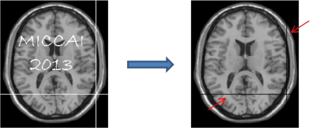
Matrix completion is widely applied to image/video in-painting and decoding problems. However, matrix completion is limited when applied to matrices with a whole missing row or column (see white horizontal and vertical lines in Fig. 1). In this case, the missing row or column will be simply filled as an arbitrary combination of other known rows or columns to keep the total rank small. This precludes the application of matrix completion to problems such as super-resolution (SR) where missing values for many rows and columns need to be recovered in the process of up-sampling a low-resolution image by a factor of 2 times or larger [4]. Note that the goal of SR is to recover the fine anatomical details from one or more low-resolution images to construct a high-resolution image. In MR applications, single-image based SR is widely used since it requires only a single input image. For example, non-local means (NLM) is broadly employed [5], sometimes with the help from other modalities [6]. In this work, we focus on recovering a high-resolution image from a single MR image.

Fig. 1.

Recovering missing values in a 2D image by using low-rank matrix completion [1]. The red arrows mark the horizontal and vertical lines that the algorithm fails to recover.

Another limitation of matrix completion algorithms is that they consider information globally from the whole image and does not exploit the local spatial consistency. Although local information may not be useful in applications such as the Netflix problem, where different rows (e.g., users) can be considered independently, it is valuable in image recovery. A solution to this problem is to integrate low-rank regularization with local regularization such as total variation [7]. By doing so, we can take advantage of both forms of regularization to harness remote information for effective image recovery and the local information to handle missing rows and columns.

Specifically, in this paper, we propose a novel low-rank total variation (LRTV) method for recovering a high-resolution image from a low-resolution image. Our method 1) explicitly models the effects of down-sampling and blurring on the low-resolution images, and 2) uses both low-rank and total variation regularizations to help solve the ill-conditioned inverse problem. Experiments on MR images of both adults and pediatric subjects demonstrate superior results of our method, compared to interpolation methods as well as NLM and TV-based up-sampling methods.

2 Method

For recovering the high-resolution image, our method 1) uses low-rank regularization to help retrieve useful information from remote regions; and 2) uses total variation regularization for keeping better local consistency.

2.1 Super-Resolution Problem

The physical model for the degradation effects involved in reducing a high-resolution (HR) image to a low-resolution (LR) image can be mathematically formulated as:

$$T=DSX+n$$ (1)

where T denotes the observed LR image, D is a down-sampling operator, S is a blurring operator, X is the HR image that we want to recover, and n represents the observation noise. The HR image can be estimated using this physical model by minimizing the below least-square cost function:

$$\underset{X}{\text{min}}{\Vert DSX-T\Vert }^2+\lambda \Re (X)$$ (2)

where the first term is a data fidelity term used for penalizing the difference between the degraded HR image X and the observed LR image T. The second term is a regularization term often defined based on prior knowledge. Weight λ is introduced to balance the contributions of the fidelity term and regularization term.

2.2 Formulation of Low-Rank Total-Variation (LRTV) Method

The proposed LRTV method is formulated as follow:

$$\underset{X}{\text{min}}{\Vert DSX-T\Vert }^2+{\lambda }_{\mathit{\text{rank}}}{\Vert X\Vert }_{*}+{\lambda }_{\mathit{\text{tv}}}TV(X)$$ (3)

where the second term is for low-rank regularization, and the third term is for total variation regularization. λ_rank and λ_tv are the respective weights.

Low-Rank Regularization

A N-dimensional image can be seen as a high order tensor, and its rank can be defined as the combination of trace norms of all matrices unfolded along each dimension [1]: ${\Vert X\Vert }_{*}={\sum }_{i=1}^N{\alpha }_i{\Vert X_{(i)}\Vert }_{\mathit{\text{tr}}}$, where N is the number of image dimensionality such as N = 3 for the 3D images. α_i are parameters satisfying α_i ≥ 0 and ${\sum }_{i=1}^N{\alpha }_i=1$. X_(i) is the unfolded X along the i-th dimension: unfold_i(X) = X_(i). For example, a 3D image with size of U × V × W can be unfolded into three 2D matrices, with size of U × (V × W), V × (W × U), and W × (U × V), respectively. ‖X_(i)‖_tr is the trace norm, which can be computed by summing the singular values of X_(i). We employ the alternating direction method of multipliers (ADMM) [8] to solve this problem.

Total-Variation Regularization

The TV regularization term is defined as the integral of the absolute gradient of the image [9]: TV(X) = ∫|∇X|dxdydz. TV-regularization is formulated based on the observation that unreliable image signals usually have excessive and possibly spurious details, which lead to a high total variation. Thus, by minimizing the TV to remove such details, the estimated image will more likely match the original image. It has been proved quite effective in preserving edges. The TV-regularization problem can be solved by split Bregman method [10].

2.3 LRTV Optimization

We follow the alternating direction method of multipliers (ADMM) algorithm to solve the cost function in Eq. (3). ADMM is proven to be efficient for solving optimization problems with multiple non-smooth terms in the cost function [8]. We introduce redundant variables ${\{M_i\}}_{i=1}^N$ to obtain the following new cost function:

$${\text{min}}_{X,{\{M_i\}}_{i=1}^N}{\Vert DSX-T\Vert }^2+{\lambda }_{\mathit{\text{rank}}}{\sum }_{i=1}^N{\alpha }_i{\Vert M_{i(i)}\Vert }_{\mathit{\text{tr}}}+{\lambda }_{\mathit{\text{tv}}}TV(X)\text{subject to}{X}_{(i)}=M_{i(i)},i=1,\dots ,N$$ (4)

Here, for each dimension i, we use M_i to simulate X by requiring that the unfolded X along the i-th dimension X_(i) should be equal to the unfolded M_i along this dimension M_i(i).

The cost function in Eq. (4) can be further rewritten as an unconstrained optimization problem by replacing the constraints between X_(i) and M_i(i) using a new term based on Augmented Lagrangian method of multiplier with multiplies ${\{Y_i\}}_{i=1}^N$ [8]:

$${\text{min}}_{X,{\{M_i\}}_{i=1}^N,{\{Y_i\}}_{i=1}^N}{\Vert DSX-T\Vert }^2+{\lambda }_{\mathit{\text{rank}}}{\sum }_{i=1}^N{\alpha }_i{\Vert M_{i(i)}\Vert }_{\mathit{\text{tr}}}+{\lambda }_{\mathit{\text{tv}}}TV(X)+{\sum }_{i=1}^N\frac{\rho }{2}({\Vert X-M_i+Y_i\Vert }^2-{\Vert Y_i\Vert }^2)$$ (5)

According to ADMM [8], we break Eq. (5) into three sub-problems below that need to be solved for iteratively updating the variables.

Subproblem 1

Update X^(k+1) by minimizing:

$$\text{arg}\underset{X}{\text{min}}{\Vert DSX-T\Vert }^2+{\lambda }_{\mathit{\text{tv}}}TV(X)+{\sum }_{i=1}^N\frac{\rho }{2}{\Vert X-M_i^{(k)}+Y_i^{(k)}\Vert }^2$$ (6)

This subproblem can be solved by gradient descent with step size dt.

Subproblem 2

Update ${\left\{M_i^{(k+1)}\right\}}_{i=1}^N$ by minimizing:

$$\underset{{\{M_i\}}_{i=1}^N}{\text{min}}{\lambda }_{\mathit{\text{rank}}}{\sum }_{i=1}^N{\alpha }_i{\Vert M_{i(i)}\Vert }_{\mathit{\text{tr}}}+{\sum }_{i=1}^N\frac{\rho }{2}{\Vert X^{(k+1)}-M_i+Y_i^{(k)}\Vert }^2$$ (7)

which can be solved using a close-form solution according to [11]:

$$M_i={\mathit{\text{fold}}}_i\left[SV{T}_{{\lambda }_{\mathit{\text{rank}}}{\alpha }_i/\rho }\right(X_{(i)}^{(k+1)}+Y_{i(i)}^{(k)}\left)\right]$$ (8)

where fold_i(·) is the inverse operator of unfold_i(·), i.e., fold_i(M_i(i)) = M_i . SVT(·) is the Singular Value Thresholding operator [11] using λ_rankα_i/ρ as the shrinkage parameter.

Subproblem 3

Update ${\left\{Y_i^{(k+1)}\right\}}_{i=1}^N$ by:

$$Y_i^{(k+1)}=Y_i^{(k)}+(X^{(k+1)}-M_i^{(k+1)})$$ (9)

Parameters are optimized based on a small set of datasets. In this work, we set α₁ = α₂ = α₃ = 1/3, λ_rank = 0.01, λ_TV = 0.01, dt = 0.1, and the maximum iteration as 200. The difference between iterations is measured by ‖X^k − X^k−1‖/‖T‖, and the program is stopped when this difference is less than ε = 1e − 5.

Algorithm 1.

Low-Rank Total Variation (LRTV) for Image Super Resolution

Input:	Low-resolution image T;
Output:	Reconstructed high-resolution image X;
Initialize:	X = upsample(T)*, M = 0, Y = 0.
Repeat
1. Update X based on Eq. (6);
2. Update M based on Eq. (7);
3. Update Y based on Eq. (9);
4. Until difference in the cost function (Eq. (5)) is less than ε;
End

^*The upsample(·) operator is implemented by nearest-neighbor interpolation.

3 Experiments

3.1 Low-Rank Representation

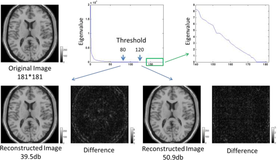
We first evaluated whether brain images can be sufficiently characterized using low-rank representations. We selected a representative 2D slice from an adult T1 MR image in Brainweb (http://www.bic.mni.mcgill.ca/brainweb/), which has a size of 181×181 and in-plane resolution of 1 mm (Fig. 2). We then performed singular value decomposition (SVD) on this image to obtain its 181 eigenvalues. As shown in Fig. 2, the eigenvalues decrease dramatically, with most values being close to zero. We reconstructed the image after removing the small eigenvalues, and compared it with the original image. Peak signal-to-noise ratio (PSNR) is used to evaluate the quality of reconstruction: PSNR = 20 * log10(‖Truth‖/‖Truth − Recovered‖).

Fig. 2.

Low-rank representation of brain images. Top row shows the original image, eigenvalue plot, and zoomed eigenvalue plot of indices from 140 to 181. Bottom row shows the two reconstructed images and their differences with the original image by using top 80 and 120 eigenvalues, respectively.

The result shows that, by using the top 80 eigenvalues, the reconstructed image has high PSNR (39.5db), although some edge information in the brain boundary is lost. However, when using the top 120 eigenvalues (out of 181), the resulting image does not show visual differences with respect to the original image. For the 3D Brainweb image with size of 181×217×181, its rank can actually be computed by the average rank of its 3 unfolded 2D images, which is thus less than its longest image size 217. This rank is very low, compared to its voxel number of 7.1×10⁶. Our analysis suggests that brain images can be represented using the low-rank approximations.

3.2 Experimental Setting

We applied our method to a set of down-sampled and blurred 3D brain images and evaluated whether our method can successfully recover the original high-resolution images (Fig. 3). Blurring was implemented using a Gaussian kernel with a standard deviation of 1 voxel. The blurred image was then down-sampled by averaging every 8 voxels (to simulate the partial volume effect), resulting in half of the original resolution. The quality of reconstruction of all methods was evaluated by comparing with the ground-truth images using PSNR.

Fig. 3.

Simulation of low-resolution image from high-resolution image

Our method was evaluated on two publicly available datasets. First, we randomly select 30 adult subjects from ADNI (http://www.loni.ucla.edu/ADNI), with 10 from Alzheimer's disease (AD), 10 from mild cognitive impairment (MCI), and 10 from normal controls. Their ages were 75±8 years at MRI scan. T1 MR images were acquired with 166 sagittal slices at the resolution of 0.95×0.95×1.2 mm³. Second, we randomly select 20 pediatric subjects from NDAR (http://ndar.nih.gov/), with age of 11±3 years at MRI scan. T1 MR images were also acquired with 124 sagittal slices at the resolution of 0.94×0.94×1.3 mm³.

3.3 Results

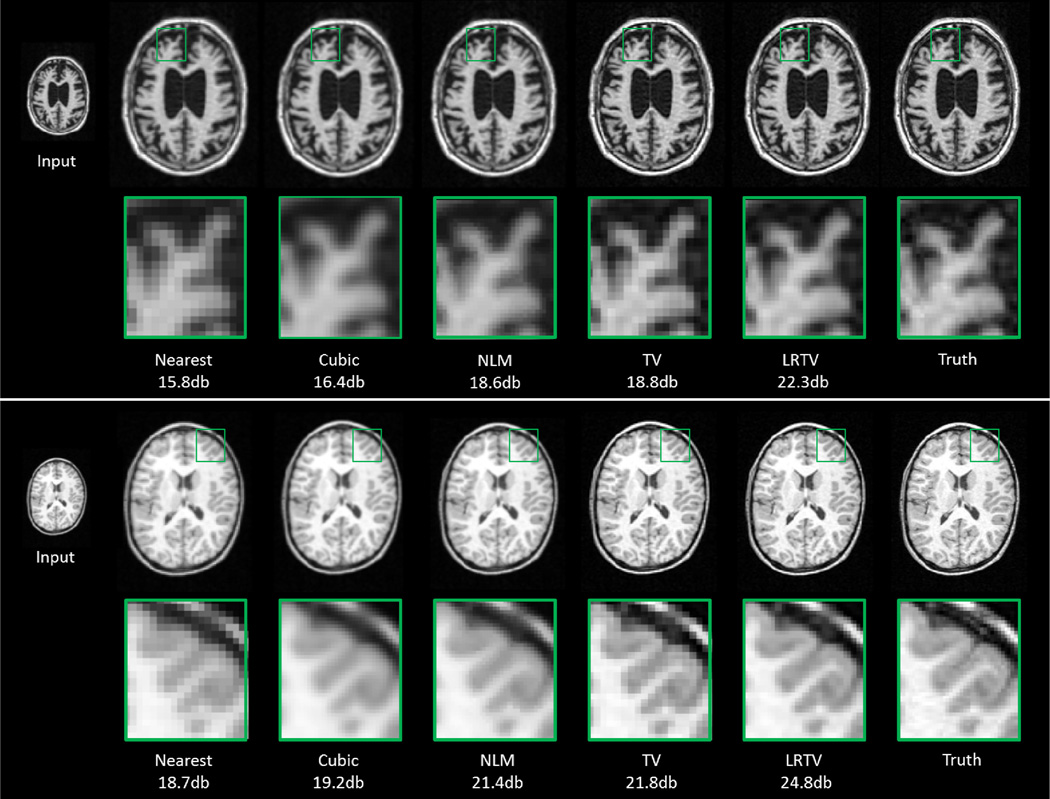
Fig. 4 shows the representative image SR results of an adult scan (upper panel) and a pediatric scan (lower panel). For the first row of each panel, from left to right show the input image, the results of nearest-neighbor interpolation, cubic interpolation, NLM based up-sampling [5], TV based up-sampling [10], proposed LRTV method, and ground truth. Of note, here we used the implementation of NLM released by authors (https://sites.google.com/site/pierrickcoupe/). We implemented TV through the proposed method by setting λ_rank = 0, ρ = 0, and solving only the subproblem 1.

Fig. 4.

Results for an adult scan (upper panel) and a pediatric scan (lower panel). In each panel, the first row is the input image and second row is the closeup view of selected regions.

Closeup views of selected regions are shown for better visualization. It can be observed that the results of both the nearest-neighbor and cubic interpolation methods show severe blurring artifacts. The contrast is enhanced in the results of NLM and TV up-sampling methods, while the proposed LRTV method preserves edges best and achieves the highest PSNR values.

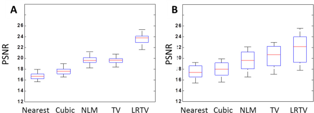
Quantitative results on the images of 30 adults and 20 pediatric subjects are shown in Fig. 5. Our proposed method significantly outperforms all other comparison methods (p<0.01). Results on adult subjects demonstrate less variance and higher accuracy than that of pediatric subjects, which may be because the image quality is higher in the matured brain and clearer gyri/sulci patterns appear in the adult images. No significant difference was found between the adult subjects of AD, MCI, and controls.

Fig. 5.

Boxplot of PSNR results for (A) adult dataset and (B) pediatric dataset. The proposed LRTV method significantly outperforms all other comparison methods (p<0.01).

4 Conclusion and Future Work

We have presented a novel super-resolution method for recovering a high-resolution image from a single low-resolution image. For the first time, we show that estimation with a combined low-rank and total-variation regularization is a viable solution to the SR problem. This combination brings together global and local information for effective recovery of the high-dimensional image. Experimental results indicate that our method outperforms the nearest interpolation, cubic interpolation, NLM- and TV-based up-sampling. It is worth noting that the interpolation methods (nearest, cubic) do not estimate the image generation process, which is the intrinsic limitation of that kind of methods. While for TV and NLM, they used the same model as the proposed method, so the comparisons are fair. Meanwhile, although our method is developed for single-image SR, it can be easily generalized to multiple-image SR. Our future work will be dedicated to extend the proposed method to longitudinal scans, i.e., images acquired from the same subject at different time points.

References

- 1.Liu J, Musialski P, Wonka P, Ye J. Tensor Completion for Estimating Missing Values in Visual Data. IEEE Transactions on Pattern Analysis and Machine Intelligence. 2013;35:208–220. doi: 10.1109/TPAMI.2012.39. [DOI] [PubMed] [Google Scholar]
- 2.Netflix: Netflix prize webpage. 2007 http://www.netflixprize.com/
- 3.Candès EJ, Recht B. Exact matrix completion via convex optimization. Foundations of Computational Mathematics. 2009;9:717–772. [Google Scholar]
- 4.Park SC, Park MK, Kang MG. Super-resolution image reconstruction: a technical overview. IEEE Signal Processing Magazine. 2003;20:21–36. [Google Scholar]
- 5.Manjón JV, Coupé P, Buades A, Fonov V, Louis Collins D, Robles M. Non-local MRI upsampling. Medical Image Analysis. 2010;14:784–792. doi: 10.1016/j.media.2010.05.010. [DOI] [PubMed] [Google Scholar]
- 6.Rousseau F. A non-local approach for image super-resolution using intermodality priors. Medical Image Analysis. 2010;14:594. doi: 10.1016/j.media.2010.04.005. [DOI] [PMC free article] [PubMed] [Google Scholar]
- 7.Chambolle A, Lions P-L. Image recovery via total variation minimization and related problems. Numerische Mathematik. 1997;76:167–188. [Google Scholar]
- 8.Boyd S, Parikh N, Chu E, Peleato B, Eckstein J. Distributed optimization and statistical learning via the alternating direction method of multipliers. Foundations and Trends in Machine Learning. 2011;3:1–122. [Google Scholar]
- 9.Rudin LI, Osher S, Fatemi E. Nonlinear total variation based noise removal algorithms. Physica D: Nonlinear Phenomena. 1992;60:259–268. [Google Scholar]
- 10.Marquina A, Osher SJ. Image super-resolution by TV-regularization and Bregman iteration. Journal of Scientific Computing. 2008;37:367–382. [Google Scholar]
- 11.Cai J-F, Candès EJ, Shen Z. A singular value thresholding algorithm for matrix completion. SIAM Journal on Optimization. 2010;20:1956–1982. [Google Scholar]