Thermal analysis of cancerous breast model

Abstract

Breast cancer is one of the most common and dangerous cancers. Subsurface breast cancer lesions generate more heat and have increased blood supply when compared to healthy tissue, and this temperature rise is mirrored in the skin surface temperature. The rise in temperature on the skin surface, caused by the cancerous lesion, can be measured noninvasively using infrared thermography, which can be used as a diagnostic tool to detect the presence of a lesion. However, its diagnostic ability is limited when image interpretation relies on qualitative principles. In this study, we present a quantitative thermal analysis of breast cancer using a 3D computational model of the breast. The COMSOL FEM software was used to carry out the analysis. The effect of various parameters (tumor size, location, metabolic heat generation and blood perfusion rate) on the surface temperature distribution (which can be measured with infrared thermography) has been analyzed. Key defining features of the surface temperature profile have been identified, which can be used to estimate the size and location of the tumor based on (measured) surface temperature data. In addition, we employed a dynamic cooling process, to analyze surface temperature distributions during cooling and thermal recovery as a function of time. In this study, the effect of the cooling temperature on the enhancement of the temperature differences between normal tissue and cancerous lesions is evaluated. This study demonstrates that a quantification of temperature distributions by computational modeling, combined with thermographic imaging and dynamic cooling can be an important tool in the early detection of breast cancer.

1. INTRODUCTION

In the U.S. and Europe, breast cancer is the most frequently diagnosed form of cancer in women [1]. In 2008, there was an incidence rate of 1.4 million cases with a worldwide mortality of 500,000 [2]. In 2012, 200,000 new cases are expected to be reported in the U.S. [3]. Breast cancer is highly treatable if it is diagnosed at an early stage [4]. The most widely used tool for breast cancer detection is mammography, but it has some significant limitations including radiation exposure, cost, patient discomfort, and more importantly, a high false positive rate. As an alternative, it is also possible to detect cancerous lesions using thermal imaging, a technique which is noninvasive and more comfortable for patient.

Although thermography has been around since the late 1950s, the mechanisms of heat transfer between diseased and native tissue and the differences between the two have yet to be well described. Previous studies indicate that tumors generate more heat than healthy tissue and this temperature change can be identified by using thermal imaging [5,6]. Despite the technological advances made with infrared imaging, thermographic imaging largely remains qualitative in nature [6] which limits its utility.

Recently researchers have used computational modeling to relate the surface temperature distribution to tumor size and location for breast cancer [7-12]. Osman and Afify (7,8) were one of the first using a hemispherical model with different tissue layers of uniform thickeness. Later Sudharsan and Ng [10,11] used models which adequately depicted the breast anatomy. Jiang et al (12) have incorporated elastic deformation in their modeling.

Mital and Pidaparti [13] and Mitra and Balaji [14] used evolutionary alogrithms and neural networks respectively to predict tumor size and location using breast thermograms. In their analysis the metabolic heat generation rate was varied with tumor diameter, whereas the blood perfurion rate of the tumor was kept constant.

In this study, we present a computational model and a quantitative analysis to provide a more accurate description of the thermal characteristics of breast cancer lesions including the dependance of the temperature distribution on size, shape, and depth of the lesion. Specifically we used a parametric analysis of the breast to obtain a set of features that can be used to predict the location and size of the breast cancer lesion from surface temperature measurements, which is essential in diagnostic applications. In order to improve thermal image acquistion procedure and ensure reproducibility and accuracy of the imaging procedure, a cooling load was applied in the analysis to enhance the thermal visibility and allow meaningful measurements of the physical and thermophysical characterisitics of the lesion. This work should allow clinicians a more accurate, noninvasive and cost effective tool in the early diagnosis of one of the most common and dangerous cancers.

2. NUMERICAL MODELING

The human breast is a multilayer structure consisting of the layers epidermis, papillary dermis, reticular dermis, fat, gland and muscle, as shown in Figure 1(a). The dimensions of these layers are given in Table 1. In order to investigate early stage cancer, the tumor diameter has been kept under 20 mm [16].

FIGURE 1.

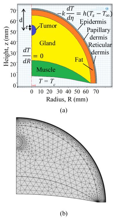
a) SCHEMATIC OF THE BREAST WITH THE TISSUE LAYERS USED IN THE COMPUTATIONAL MODEL

(b) THE COMPUTATIONAL MESH GENERATED

TABLE 1.

THERMOPHYSICAL PROPERTIES

	Epidermis [15]	Papillary Dermis [15]	Reticular Dermis [15]
h (mm)	0.1	0.7	0.8
k (W/m.K)	0.235	0.445	0.445
ρ (kg/m3)	1200	1200	1200
c (J/kgK)	3589	3300	3300
Q (W/m3)	0	368.1	368.1
ωb (m3/s/m3)	0	0.0002	0.0013

	Fat	Gland	Muscle	Tumor
h (mm)	5.0[10]	43.4[10]	15 [10]	--
k (W/mK)	0.21 [11]	0.48 [11]	0.48 [11]	0.48 [11]
ρ (kg/m3)	930 [18]	1050 [18]	1100 [18]	1050 [18]
c (J/kgK)	2770 [18]	3770 [18]	3800 [15]	3852 [15]
Q (W/m3)	400 [11]	700 [11]	700 [11]	5000 [12]

The breast has been modeled as a hemisphere with layers shown in Fig. 1. The Pennes bioheat equation [17] was used to model heat transfer in the breast tissue. The Pennes bioheat equation for the n^th layer is given by

$${\rho }_n{c}_n\frac{\partial T}{\partial t}=k_n{\nabla }^{2}T+{\rho }_b{c}_b{\omega }_b(T_b-T_n)+Q_n$$ (1)

where ρ_b, c_b, T_b and ω_b represents density, specific heat of blood, arterial temperature and blood perfusion rate respectively. Tissue properties density, specific heat, temperature, thermal conductivity and metabolic heat generation are given by ρ, c, T, k and Q. These properties are listed in Table 1. The blood perfusion rate (ω_b) for fat, gland, muscle and tumor is taken as 0.0002 m³/s/m³ , 0.0006 m³/s/m³ , 0.0009 m³/s/m³ and 0.012 m³/s/m³ respectively. These values are close to the values used by Ng and Sudharsan [11].

Heat flux and temperature continuity at the interface of the tissue layers is described by equations

$$k_n\frac{\partial T_n}{\partial \eta }=k_{n+1}\frac{\partial T_{n+1}}{\partial \eta }$$ (2)

$$T_n=T_{n+1}$$ (3)

respectively. In Eq. (2). η is the direction perpendicular to the surface. The lower part of the muscle layer is assumed to be at a core body temperature

$$T=T_C=37°C.$$ (4)

Due to the axisymmetric nature of the problem with a lesion symmetrical around the axis, the left boundary (axis) is described by the symmetry boundary condition

$$\frac{\partial T}{\partial r}=0\mathit{at}r=0$$ (5)

At the skin surface convective boundary condition is used

$$-k\frac{\partial T}{\partial \eta }=h(T_s-T_{\infty })$$ (6)

where: k= 0.235 Wm⁻¹K⁻¹, h = 10 Wm⁻²K⁻¹, T_∞ = 21 °C

In the transient analysis the surface is cooled using constant temperature boundary condition (Eq. (7).)

$$T\left(t\right)=T_{\mathit{cooling}}0<t<t_{\mathit{cooling}}$$ (7)

The commercial software COMSOL Multiphysics v 4.2 (2011) [19] was used to solve these equations. The mesh generated in COMSOL is displayed in Fig. 1b. The mesh is finer for thin layers (epidermis, papillary dermis and reticular dermis) compared to other layers.

In order to ensure the mesh independence we tracked the temperature of a point on the axis located on the surface and the average surface temperature. The grid points were varied from 5000 to 29000 and the temperature difference was less than 0.1%. To ensure that the transient analysis is independent of the time step, the surface temperature at the axis was tracked. The variation in temperature was less than 0.1% when the time step was varied from 0.1 seconds to 2 seconds. Hence a mesh with 7800 grid points and a time step of 1 s (the time step was 0.1 s for the initial 10 s) were used.

3. RESULTS AND DISCUSSION

In this section computational simulation results are presented and discussed. The analysis is divided into two parts, steady state and transient. In steady state analysis the effect of tumor size and location on the surface temperature is studied. Based on this analysis two key features were identified, which can be used to predict the tumor characteristics. In addition, a parametric study is carried out to investigate the effect of blood perfusion rate and metabolic heat generation rate of the tumor on the surface temperature. Then the model is compared with experimental data. The second part of this section focuses on the transient analysis and the propagation of the cooling effect into the tissue. The effect of cooling time and cooling temperature on the thermal contrast on the skin surface, obtained during recovery phase, is analyzed.

3.1 Steady State Analysis

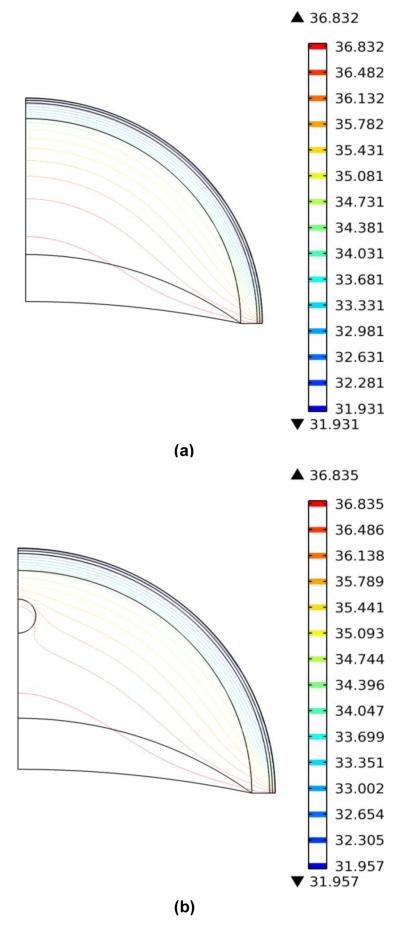
Figure. 2(a) shows the isotherms for the cross section in the normal breast during steady state. The temperature decreases through the tissue towards the skin surface. The isotherms for cancerous breast are shown in Fig. 2(b). Near the tumor the isotherms become distorted and indicate that the tumor has higher temperature when compared to the normal tissue. This increase in temperature is also visible on the skin surface.

FIGURE 2.

a) ISOTHERMS FOR NORMAL BREAST

(b) ISOTHERMS FOR CANCEROUS BREAST

3.1.1 Effect Of Tumor Size And Depth

The surface temperature, T, along the circumference of the breast is displayed in Fig. 3. The surface temperature profiles for different sizes (r, tumor radius) and locations of the tumor (d, depth beneath the skin surface) are plotted along with the temperature profile for a normal case. The results suggest that there is temperature increase in the range from 0.1°C to 0.8°C, and these increases can be accurately measured by modern infrared cameras. The difference in temperature, ΔT, between the cancerous and normal (without lesion) case (bottom blue line in Fig. 3) is plotted in Fig. 4 to analyze the effect of tumor. As expected, for an axisymmetric tumor, the maximum temperature rise, ΔT_max, is detected at the axis. For a fixed tumor radius of 5 mm, the maximum temperature difference increased from 0.08 °C to 0.58 °C as the depth of tumor is decreased from 20 mm to 10 mm. Similarly, for a fixed depth of 15 mm, the maximum temperature difference increased from 0.03 °C to 0.50 °C as the radius of the tumor is increased from 2.5 mm to 7.5 mm. All other properties remained the same.

FIGURE 3.

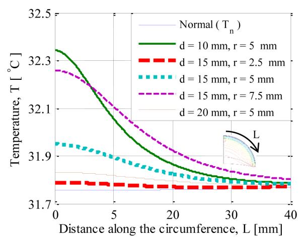
SURFACE TEMPERATURE DISTRIBUTION FOR TUMOR RADIUS r AND TUMOR DEPTH d AS PARAMETERS

FIGURE 4.

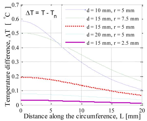
SURFACE TEMPERATURE INCREASE FOR TUMORS RADIUS r AND TUMOR DEPTH d AS PARAMETERS

The dependence of the maximum temperature difference on tumor size and depth is shown in Fig. 5. The result agrees with the observation made by Amri et al [17] that the presence of tumor is always accompanied with an increase in surface temperature. The temperature rise might be very small but it is always present even for very a small tumor. It is clear from the Fig.5 that as the tumor size increases for fixed depth and as the depth of the tumor decrease for fixed diameter, the maximum temperature difference increases.

FIGURE 5.

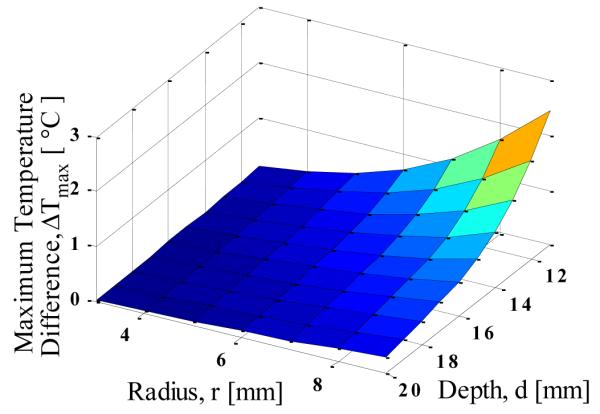
MAXIMUM TEMPERATURE DIFFERENCE AS FUNCTION OF TUMOR SIZE AND DEPTH

According to a similar analysis done by Amri et al. [17] and Jiang et al. [12], they obtained negligible variation in maximum temperature difference with varying tumor size. In their analysis they used equation

$$\mathrm{Q}=\mathrm{C}∕(468.6\ln 200\mathrm{r}+50)$$ (8)

to calculate metabolic heat generation from the diameter of the tumor According to this expression, the metabolic heat generation rate decreases with increasing size. Due to this decrease, the effect of increasing size of tumor is countered by the decreasing metabolic heat generation rate, and therefore there is no significant change in maximum surface temperature as the size of the tumor varies. Therefore, the mismatch between the result obtained here and the one given in literature is due to the variation in metabolic heat generation rate. In order to do a comprehensive analysis we are not assuming that the metabolic heat generation rate is related to the tumor diameter. We treat it as an independent parameter, which is more consistent with the real life situation: both large and small tumors can be aggressive and have large metabolic heat generation rates, and vice versa.

While Fig. 5 is helpful in understanding the behavior of maximum temperature rise as the depth and size of the tumor is varied, this result alone cannot be used to estimate the location and size of the tumor. The analysis suggests that the same maximum temperature rise can be observed for different combinations of tumor depth and size.

The results in Fig. 4 indicate that the slope of the temperature difference curve increases (it becomes steeper) with decreasing tumor depth. Here ‘half temperature difference length’ (L_T), is used as a measure of this slope. It is defined as the distance from the axis along the circumference at which the temperature difference drops to half of its maximum value. As the slope of the temperature profile increases, the corresponding L_T decreases. Figure. 6 shows the variation of the half temperature difference with size and depth of the tumor, and the results indicate that L_T decreases with decreasing depth and radius. When L_T is used along with maximum temperature difference, the location and size of the tumor can be estimated. The size and depth of the tumor are the only variables in this analysis, and metabolic heat generation and blood perfusion rate were kept constant.

FIGURE 6.

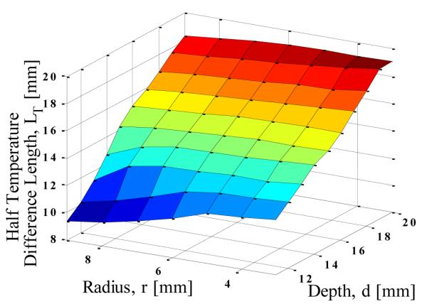
THE HALF TEMPERATURE DIFFERENCE LENGTH (A MEASURE OF THE SLOPE) AS FUNCTION OF TUMOR SIZE AND DEPTH

3.1.2 Off-Axis Tumors

In the foregoing analyses, we largely considered tumors that were symmetrical around the axis. In this section off-axis tumors are analyzed by varying the polar angle of the tumor. The computational model is three dimensional. Fig. 7 shows the surface temperature distribution for tumors with polar angles of 0°, 30° and 60°. It can be seen that the region with maximum temperature moves away from the center as the polar angle of the tumor increases. This can be seen more clearly in Fig. 8, which shows the temperature along the circumference for different positions of the tumor. The polar angle of the maximum temperature location is equal to that of the tumor.

FIGURE 7.

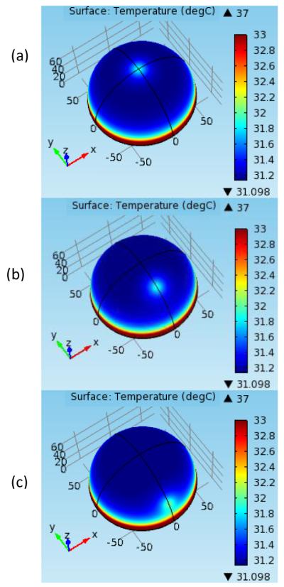
SURFACE TEMPERATURE DISTRIBUTION FOR TUMORS WITH POLAR ANGLES (a) 0° (b) 30° (c) 60°

FIGURE 8.

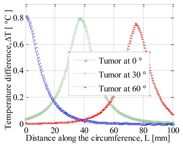
SURFACE TEMPERATURE ALONG THE CIRCUMFERENCE FOR OFF-AXIS TUMORS

3.1.3 Parametric Variation

The effect of blood perfusion rate and metabolic heat generation on the surface temperature difference (increase in surface temperature due to the presence of tumor) has been analyzed in Fig. 9. With increasing blood perfusion rate and metabolic heat generation the temperature difference increases. When the blood perfusion rate is quadrupled, from 0.006 sec⁻¹ to 0.024 sec⁻¹, the temperature difference at the axis increases from 0.4 °C to 0.8 °C. When the metabolic heat generation rate is quadrupled from 2500 W/m³ to 10000 W/m³ the temperature difference increases by 0.05 °C. It can be seen that blood perfusion rate has much more impact on the surface temperature distribution than the metabolic heat generation rate. It can also be concluded that the surface temperature is more sensitive to the variations of the blood perfusion rate than to the metabolic heat generation rate.

FIGURE 9.

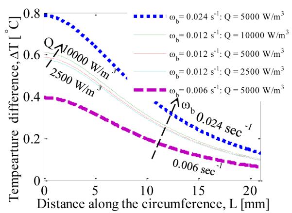
VARIATION IN SURFACE TEMPERATURE DISTRIBUTION WITH VARYING BLOOD PERFUSION RATE AND METABOLIC HEAT GENERATION RATE

3.1.4 Comparison With Experimental Data

The model is compared with the experimental data obtained by Gautherie [20]. In this comparison the thermophysical properties, geometry and boundary conditions have been taken from Mitra and Balaji [14]. Here the breast is modeled as a hemisphere of 90 mm radius.,with the tumor of 23 mm diameter at a depth of 20 mm . The heat transfer coefficient was taken as 5 W/m² and the bottom of the breast was exposed to a constant temperature (core body temperature) boundary condition. Figure 10 shows the comparison of the computational results obtained here using COMSOL and the experimental data. Though there are some differences quantitatively there is a satisfactory qualitative match.

FIGURE 10.

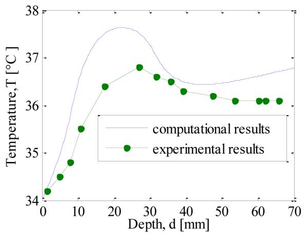
COMPARISON OF THE COMPUTED DATA WITH EXPERIMENTAL DATA

3.2 Transient Analysis

In this section the effect of the application of cooling load, also called thermostimulation, and the subsequent recovery phase (thermal response when the cooling load is removed), is analyzed. Factors affecting the magnitude of the thermal contrast during recovery phase are investigated.

3.3.1 Cooling Phase

Figure 11. shows the axial temperature profile during the cooling phase. The constant temperature boundary condition is applied for cooling and due to this the temperature at the surface is at 14 °C during cooling. As the time progresses the temperature below the surface decreases with increasing cooling time. To obtain an estimate of the extent of the cooling, the cooling penetration depth has been defined as the maximum distance from the surface for which the drop in temperature is more than 0.3 °C. Figure. 12 shows the variation in cooling penetration depth with time. As expected, the cooling depth increases with increasing cooling time.

FIGURE 11.

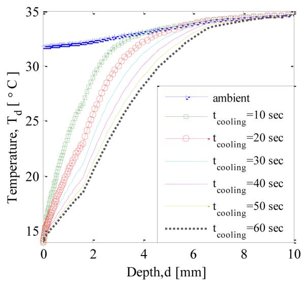
TEMPERATURE PROFILE ALONG THE AXIS DURING COOLING

FIGURE 12.

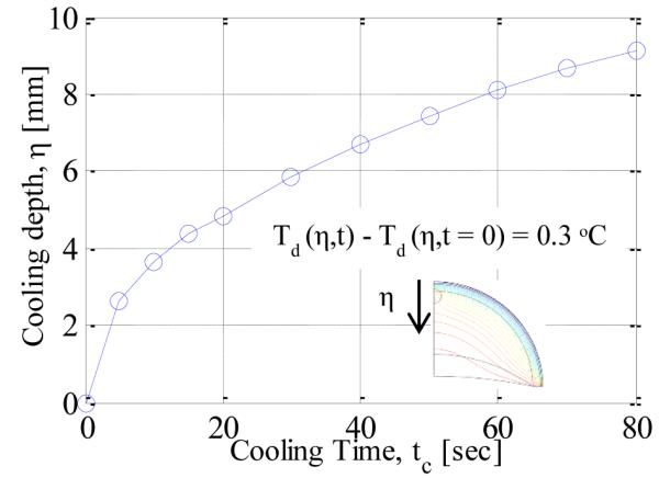
COOLING DEPTH VS. COOLING TIME

3.3.2 Thermal Recovery Phase

Axial Temperature Profile

After the cooling load is removed, the temperature gradually increases and over time reaches the steady state condition. Figure 13. shows how the axial temperature changes after the cooling load is removed. It can be seen that, as the time progresses, the temperature profile approaches the steady state condition (no cooling load). The temperature of the tissue increases gradually after removing the cooling load. When the temperature profiles, just after removal of cooling and 50 seconds later, are compared, it is observed that the temperature of the region which is within 3 mm from the surface (towards the left of point A) experiences a decrease in temperature, whereas the deeper regions are still undergoing cooling. Similarly, when comparing temperature profiles at 50 seconds and 200 seconds, the region which is deeper than 6 mm is still undergoing cooling. Therefore it can be concluded that there is a time lag between removal of cooling load and rising of the temperature in the tissue and thus the cooling depth keeps on increasing even after removing the cooling load.

FIGURE 13.

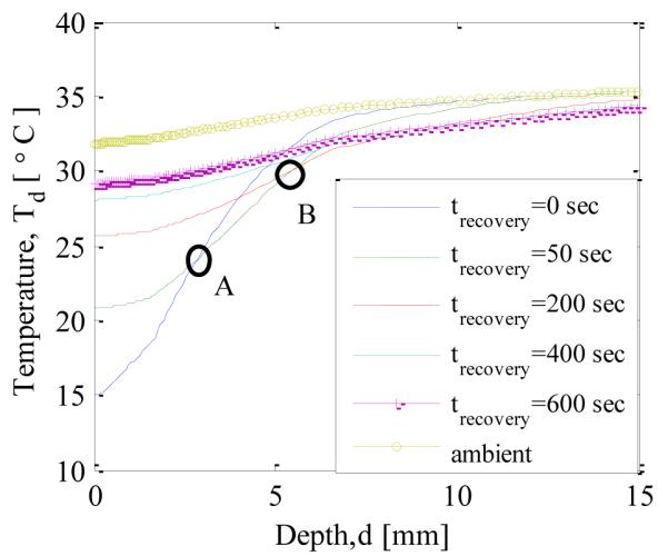
TEMPERATURE PROFILE ALONG THE AXIS DURING RECOVERY AFTER 60 s OF COOLING

Recovery Profile

In Fig. 14 the surface temperature just above the tumor (on the axis) is plotted as a function of time during the thermal recovery phase for the normal and cancerous case. It should be noted that the plotted temperature is from the location which has the maximum temperature rise. The difference between the two profiles is indicated on the right axis. Constant temperature of 14 °C was applied during cooling, and therefore the recovery curve starts from 14 °C for both the cases. It can be seen that the difference between the two temperature profiles reaches a maximum of 0.9 °C after 10 minutes, and this time will be referred to as ‘peak time’(t_p). The difference gradually stabilizes to 0.6 °C which is the steady state temperature difference. It can be seen that the temperature contrast increases by 0.3 °C due to the application of cooling load.

FIGURE 14.

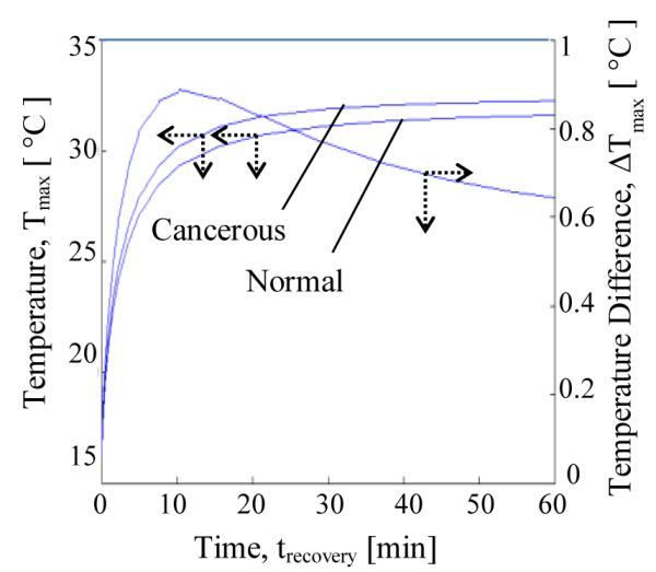
THE EFFECT OF TUMOR ON THE TEMPERATURE DIFFERENCE VS. TIME GRAPH DURING RECOVERY PHASE

Effect Of Cooling Load

In this section the effect of cooling load on the thermal recovery profile is analyzed. Two cooling methods are considered: constant temperature cooling and convective cooling. When the cooling time, for constant temperature cooling, is increased from 10 seconds to 80 seconds the maximum temperature difference during recovery, Δ T_max,recovery, increases from 0.7 °C to 0.9 °C (Fig. 15). When the cooling temperature is reduced from 20 °C to 14 °C for the constant temperature cooling case the maximum temperature difference increases from 0.75 °C to 0.9 °C (Fig. 16). For the convective cooling situation the maximum temperature difference increased from 0.60 °C to 0.65 °C when cooling time was increased from 30 seconds to 120 seconds (Fig. 15). When the cooling temperature is decreased from 20 °C to 14 °C for the convective cooling case the maximum temperature difference increases from 0.60 °C to 0.62 °C (Fig. 16). The increase in maximum temperature difference is more for constant temperature cooling as compared to convective cooling.

FIGURE 15.

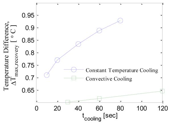
EFFECT OF COOLING TIME ON THE MAXIMUM TEMPERATURE DIFFERENCE

FIGURE 16.

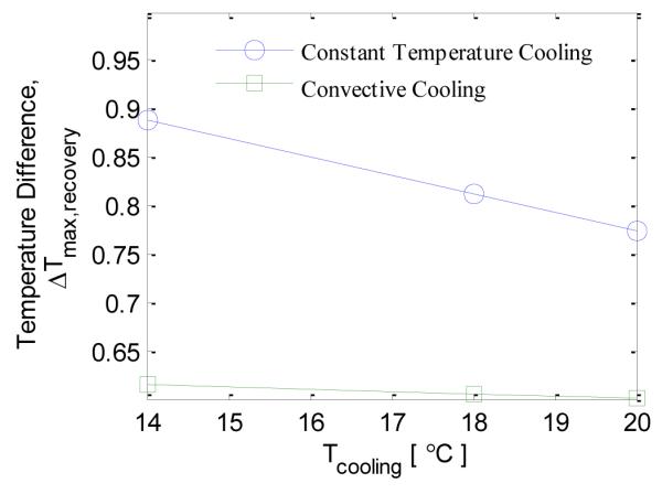
EFFECT OF COOLING TEMPERATURE ON THE MAXIMUM TEMPERATURE DIFFERENCE

3.3 Key Features To Predict Size And Location Of The Tumor

As mentioned in section 3.2.1 there are two key features of the surface temperature profile relevant for predicting lesion properties: maximum temperature difference and half temperature difference length. By using these two features it is possible to estimate the location and size of the tumor. It should be noted that the blood perfusion rate and metabolic heat generation rate are known quantities in the analysis. Further, only axisymmetric case was considered.

It was also observed that for off-axis tumors the polar angle of the tumor can be determined using surface temperature profile. Using this observation and the above mentioned features, it is possible to extend this analysis for a general case of off-axis tumors.

4. CONCLUSIONS

In the present work a three-dimensional model of the breast was introduced and solved for temperature distribution under various conditions using COMSOL. The surface temperature distribution for various sizes and locations of axisymmetric tumors was analyzed. The behavior of off-axis tumors was analyzed next, and it was shown that the polar location of the tumor can be predicted using the surface temperature profile. The parametric analysis during steady state conditions predicts that the variation in surface temperature profile due to metabolic heat generation is negligible as compared to blood perfusion rate.

It is observed by means of transient analysis that the cooling depth increases even after removing the cooling load. The effect of cooling load on the recovery profile was analyzed and it was found that as the cooling time increases and cooling temperature decreases the highest temperature difference increases for both constant temperature cooling and convective cooling. Constant temperature cooling is far more effective than convective cooling.

Based on the steady state analysis two key features, maximum temperature difference and half temperature difference length were identified as data allowing to estimate the location and size of the tumor from the surface temperature distribution. In this analysis metabolic heat generation and blood perfusion rate were assumed to be known quantities. Though the analysis was conducted for the axisymmetric case, it can be extended to off-axis tumors based on the observation that the polar angle of the tumor can be estimated using the surface temperature distribution.