Climate change, humidity, and mortality in the United States

Abstract

This paper estimates the effects of humidity and temperature on mortality rates in the United States (c. 1973–2002) in order to provide an insight into the potential health impacts of climate change. I find that humidity, like temperature, is an important determinant of mortality. Coupled with Hadley CM3 climate-change predictions, I project that mortality rates are likely to change little on the aggregate for the United States. However, distributional impacts matter: mortality rates are likely to decline in cold and dry areas, but increase in hot and humid areas. Further, accounting for humidity has important implications for evaluating these distributional effects.

1. Introduction

The Earth’s climate is expected to become hotter and more humid in the coming century due to man-made pollution. The goal of this paper is to quantify how these climatic changes will affect human health conditions in the United States. Although previous research has estimated the potential health costs of higher temperatures (e.g., Deschênes and Greenstone [1]), this study is the first to examine the impact of rising humidity levels. I use a within-county identification strategy to estimate the effects of humidity and temperature on monthly mortality rates over a 30-year period (c. 1973–2002). I then make end-of-the-21st-century projections using my mortality estimates and a “business-as-usual” scenario from the Hadley CM3 climate model. In addition to contributing to the evaluation of optimal climate-change mitigation policies, my research adds to the literature on the importance of the weather, and in particular humidity, as a determinant of human health and welfare.

The expected net effect of climate change on mortality is ambiguous prima facie. Exposure to extreme temperatures and/or extreme humidity levels increases the risk of mortality mostly through impacts on the cardiovascular and respiratory systems. Due to greenhouse gas emissions, climatologists predict that the Earth’s climate will warm in the coming century. As a result of this warming, the weather is expected to become “more extreme” during summer months (e.g., hotter and more humid) but “less extreme” during winter months (e.g., less cold and less dry).¹ Thus, mortality rates are likely to increase during summer months but decrease during winter months. In simple terms, this study determines the net effect of these climatic changes on mortality.

In this paper, I make two key contributions to the literature: first, I provide comprehensive estimates of the effects of humidity and temperature on mortality in addition to estimating the effects of temperature on mortality. As Schwartz et al. [5] note, “the effects of humidity on mortality have received little investigation.” Conversely, the effects of temperature have received much attention in the literature.² Also, unlike my study, those humidity-mortality studies that do exist are subject to concerns of external validity because of small sample sizes.

For the second contribution of this paper, I incorporate the effects of humidity when forecasting the effects of climate change on mortality rates in the United States. My study builds on recent research by Deschênes and Greenstone [1] (hereafter DG) who examine the impact of changing temperatures on mortality rates in the United States. In short, they present compelling evidence that the temperature-mortality relationship is U-shaped. Using climate-change predictions from the Hadley CM3 climate model, DG project that mortality rates will increase by almost 2% in the coming century. However, DG’s results are potentially biased because they fail to control for humidity.

The mortality data and the weather data used in my analysis were constructed from the National Center for Health Statistics’ Multiple Causes of Death (MCOD) files and the National Climatic Data Center’s Global Summary of the Day (GSOD) files. The MCOD files provide mortality counts for counties with over 100,000 inhabitants. I construct county-by-month mortality rates using the MCOD files and population estimates from the National Cancer Institute. The GSOD files are organized by weather station and day. The key weather variables of interest are daily mean temperature and daily mean specific humidity. I aggregate the station-day data to the county-month level using inverse-distance weights between the station and the geographic centroid of each county. My sample consists of 373 well-populated counties and spans the 1973–2002 period.

There are three main components to my identification strategy: first, I include a robust set of fixed effects, like county-by-calendar-month fixed effects, in order to disentangle the causal effects of weather from other important factors that might be related to the climate. Second, I use a two-month moving average in order to account for potential inter-temporal effects of weather on mortality. Third, the effects of temperature and humidity are allowed to vary semi-parametrically so that weather “extremes” (e.g., temperatures above 90 °F) can have relatively larger impacts on mortality. In addition, I incorporate temperature – humidity interaction terms since high humidity levels may exacerbate the adverse effects of hot temperatures.

It is important to highlight the limitations of my research design in the context of measuring the impacts of climate change. On one hand, my study may overstate the costs of climate change because the estimates are derived from unanticipated weather shocks. Individuals may be able to mitigate future costs by adopting health-saving technologies (e.g., dehumidifiers) or by migrating to more favorable climates. On the other hand, my study may understate the health impacts of climate change because the welfare calculations ignore morbidity, weather-related natural disasters (e.g., hurricanes), other health inputs (e.g., agriculture yields), or the emergence of climate-dependent diseases (e.g., malaria). Although vital for devising optimal climate-change policies, a detailed examination of these eventualities is outside the scope of my study and must be left for future research.

There are three results from my analyses that have important implications for public-health policy: first, both temperature and humidity are meaningful determinants of mortality. Specifically, the temperature – mortality relationship and the humidity – mortality relationship are both U-shaped and large in magnitude at the extremes. Low humidity levels are especially dangerous. Second, temperature and humidity have a large impact on cardiovascular- and influenza-related mortalities. To my knowledge, this is the first study to convincingly document the humidity – mortality relationship using a nationally representative sample.

Third, my study suggests that individuals are potentially under-protecting themselves from low-humidity levels. Although the focus of this paper is on mortality, I also find that energy consumption is responsive to temperature changes, but not to humidity changes. Future research should evaluate the costs and benefits of humidifying technologies in order to determine if public-health interventions are necessary. As a secondary contribution of this paper, I also project the potential impacts of climate change on energy consumption since heating, cooling, dehumidification, and humidification are important “health-related” costs of climate change.

Using climate-change predictions from the “business-as-usual” scenario (A1F1) in the Hadley CM3 climate model, I project that mortality rates are likely to fall by 0.1% on the aggregate in the United States by the end of the 21st century. However, the distributional impacts matter: hot and humid areas, like the South, will experience increases in mortality rates; cold and dry areas, like the North, will see declines in mortality rates.

Without controlling for humidity, I project a 0.9% decline in mortality rates, suggesting that omitting humidity leads to finding that climate change will have a more favorable impact on mortality than in actuality. Moreover, controlling for humidity has particularly important implications for evaluating the distributional effects of climate change. When humidity is omitted, the costs of climate change are underestimated in areas with hot and humid climates, like the South. This fact suggests that the adverse effects of climate change are going to be borne even more disproportionately by poorer areas of the United States than predicted by past research. Consequently, incorporating the effects of humidity has important implications for devising equitable climate-change policies.

On the whole, my results suggest that humidity, like temperature, is an important determinant of human health and welfare. To the extent possible, future research should account for increasing humidity levels when evaluating both the effects of climate change as well as potential mitigation strategies.

2. Understanding humidity

In broad terms, humidity refers to the amount of water vapor in the air. Two of the most commonly used measures of humidity include specific humidity and relative humidity. Specific humidity is defined as the number of grams of water vapor in a one-kilogram parcel of air. Relative humidity is the actual water vapor in the air relative to the amount of water vapor that the air could hold before saturation. These two measures are highly correlated when controlling for temperature because of their physical and mechanical relationships. For example, the actual water vapor in the air enters into the numerator in both the specific humidity and the relative humidity formulas. Consequently, the models that include both the measures of humidity risk identification off functional form assumptions and/or measurement error.

I opt to include specific humidity in my core specification since relative humidity is mechanically determined by temperature. That is, the air’s saturation point, which is the denominator in the relative humidity equation, is positively related to the temperature. Thus, measurement error in temperature readings will be negatively correlated with measurement error in relative humidity. Importantly, this non-classical measurement could bias the estimated effects of temperature and relative humidity. This argument for using specific humidity notwithstanding, my climate-change estimates are robust to controlling for relative humidity. For simplicity, I use “humidity” interchangeably with “specific humidity”, my preferred measure, for the remainder of the paper.

Specific humidity is an increasing function of the temperature and the stock of surface water. Water is more likely to turn from liquid to vapor as the temperature increases. Conditional on the temperature, the amount of water vapor in the air increases when there is more surface water because the stock of potentially evaporable water molecules is greater. As a simple illustration, Fig. 1 shows the raw correlation between daily mean temperature and daily mean specific humidity in New Orleans and Phoenix, respectively, in 2002. As hypothesized, there is a positive relationship between temperature and humidity in both cities. Conditional on temperature, New Orleans has higher humidity levels than Phoenix since New Orleans is mostly surrounded by water and Phoenix is located in the desert.

Fig. 1.

Daily mean temperature (°F) and daily mean specific humidity (g/kg), New Orleans and Phoenix, by day, 2002 only.

The fact that temperature and specific humidity are physically related has three important implications for identification. First, the models that estimate the effect of temperature on mortality without controlling for specific humidity are potentially biased. The magnitude of the bias is a function of geographic differences in the temperature – humidity gradient and changes in the temperature – humidity gradient over time. At the extreme, there would be no bias from omitting humidity if the temperature – humidity gradient was identical everywhere and fixed over time. In reality, the potential for bias is non-negligible since (a) the temperature – humidity gradient varies geographically, as illustrated by Fig. 1, and (b) the temperature – humidity gradient may vary over time due to changes in the frequency, intensity, and distribution of rainfall.³ Second, humidity may be an important mechanism through which temperature changes affect human health conditions. Thus, distinguishing the independent effects of humidity from temperature will help inform optimal public-health policies (e.g., encouraging the use of dehumidifiers), and ultimately enhance our ability to mitigate the costs of climate change.

Third, the models that control for both temperature and specific humidity are identified both by cross-sectional differences and by changes in the temperature – humidity gradient over time. Studies with small sample sizes, like many previous epidemiological studies, are likely to have little identifying variation from which to distinguish the effects of specific humidity from temperature. For example, Braga et al. [6] and Schwartz et al. [5] rely on mortality data on only 12 cities. My study overcomes this challenge using 30 years of monthly data for 373 well-populated and nationally representative counties from the United States.

3. Relationship between temperature, humidity, and mortality

Extreme temperatures are dangerous because they place stress on the cardiovascular, respiratory, and cerebrovascular systems. Breathing cold air can lead to bronchial constriction [7]. In general, previous studies have noted that cold temperatures have a larger impact on mortality than hot temperatures. Hot temperatures are more likely to affect the inter-temporal distribution of mortality by expediting the time-to-death of those individuals already nearing death, a phenomenon known as “harvesting” [8].

Humidity can affect human health through a variety of mechanisms. On one hand, low-humidity levels can lead to dehydration and promote the spread of airborne diseases, like influenza [9–11]. On the other hand, high-humidity levels exacerbate the effects of heat stress because humidity impairs the body’s ability to sweat and cool itself [12]. High-humidity levels can also affect respiratory health since they promote the spread of bacteria, fungi, and dust mites [13]. Despite these hypothesized mechanisms, the impacts of humidity on mortality have not been well established in the epidemiological literature [5].

In sum, both the temperature – mortality relationship and the humidity – mortality relationship are likely nonlinear. Therefore, I use an empirical specification that allows the mortality effects to vary depending on whether the temperature or humidity falls in one of several 10 °F or two-grams-of-water-vapor bins, respectively. Also, I include temperature – humidity interactions to test whether high-humidity levels significantly exacerbate the adverse effects of high temperatures.

4. Data

4.1. Global summary of the day

The Global Summary of the Day (GSOD) files report detailed climatic information by weather station and day and is available from 1928 through the present (National Climatic Data Center [28]). I restrict my sample to the 1973–2002 period since, as noted by the National Climatic Data Center, the “[GSOD] data from 1973 to the present [is] the most complete”. For example, a significant number of stations enter the GSOD data in 1973.⁴ Also, prior to 1973 relatively few weather stations recorded total precipitation, although these stations did record whether there was any rainfall. Thus, in order to mitigate biases from measurement error, I restrict my sample to the balanced panel of stations over the 1973–2002 period.⁵

Daily weather variables in the GSOD files include mean temperature, mean dew point, mean station pressure, and total precipitation, among other things. Although not reported in the GSOD files, I calculate mean specific humidity using a standard meteorological formula and information on mean dew point and mean station pressure. From the GSOD station-day data, I construct (aggregated) county-month weather variables using 50-mile inverse-distance weights (Hanigan et al. [25], Rising [29]). Also, I drop approximately 100 county-months where the temperature and/or humidity readings are missing for over half the month. The final dataset includes 133,793 county-months.⁶

4.2. Multiple causes of death

The MCOD data files are full censuses of the deaths that occurred in the United States (National Center for Health Statistics [27]). These data are available from 1968 to the present. I first construct all-cause and cause-specific mortality counts by county of residence and month of death. I then calculate county-by-month mortality rates per 100,000 inhabitants using state-year population estimates from the National Cancer Institute [26]. For a separate set of analyses presented in an Appendix posted to the Journal of Environmental Economics and Management’s online repository (http://www2.econ.iastate.edu/jeem/supplement.htm), I also construct county-month mortality rates by different age groups.

Due to data constraints, I rely on a select sample of counties in the MCOD data. Subsequent to 1989, counties with fewer than 100,000 inhabitants are not identified in the public-use MCOD data. I first restrict my sample to the 405 counties that have mortality data over the entire 1973–2002 period. I drop an additional 32 counties that do not have a GSOD weather station within 50 miles of the county centroid. My final sample consists of 373 counties. Though my sample consists of only 12% of the (3100+) counties in the United States, these 373 counties represented close to 70% of the entire population of the United States as of 2000. My results are qualitatively similar when I use a state-level model that includes the full sample of deaths in the MCOD data (see online Appendix Fig. 4).

Appendix Figure 4.

Mortality estimates using a state-month model

Notes: See the notes to Figure II. The state-month model includes state-by-calendar-month quadratic time trends, state fixed effects, and unrestricted year-month fixed effects.

4.3. Climate-change predictions

I use climate change predictions from the British Atmospheric Data Center [23]. Following DG, I rely on the “business-as-usual” (A1F1) scenario predictions of the Hadley CM3 climate model for the years 2070 through 2099. The Hadley CM3 model predictions are widely used by climate-change researchers.⁷ Also, the business-as-usual scenario assumes there is little or no additional effort (e.g., policy initiatives) to mitigate man-made pollution. The Hadley CM3 model reports daily mean temperature, daily specific humidity, and total precipitation at grid points across the United States that are separated by 2.5° latitude and 3.75° longitude. I construct county-level data from the Hadley predictions using inverse-distance weights of the four closest grid-points to the county centroid. In order to be consistent with the GSOD data, I restrict my sample to the 373 counties used in my core analyses. I aggregate the Hadley predictions for these 373 counties to the national-, division-, and state-level using the county population in 2000 as weights U.S. Census Bureau [31].

Next, I correct for historical and/or aggregation biases in the Hadley CM3 predictions. I construct these “bias-corrected” predictions by taking the differences between actual weather observations in the GSOD data and predictions from the Hadley CM3 data for the years 1990 through 2002; note that 1990 is the earliest year for which Hadley CM3 data exist. I add these differences back to the Hadley CM3 predictions for the 2070–2099 period. One complication with this thought-experiment is that the “bias correction” is driven by short-term weather fluctuations over the 1990–2002 period. Thus, I also present the “uncorrected” climate change predictions as an alternative scenario. Finally, I take the difference between the GSOD data (c. 1973–2002) and both the bias-corrected and uncorrected Hadley predictions (c. 2070–2099), respectively, in order to forecast end-of-the-21st-century climatic changes.

5. Estimation strategy

5.1. The reduced-form model

I estimate the effects of temperature and humidity on mortality via ordinary-least-squares using the following model:

$${\mathit{MORT}}_{\mathit{cmy}}=\sum _b{\beta }^b{\mathit{TEMP}}_{\mathit{cmy}}^b+{\sum }_{b^{\prime }}{\propto }^{b^{\prime }}{\mathit{HUMID}}_{\mathit{cmy}}^{b^{\prime }}+X_{\mathit{cmy}}\partial +{\mu }_{my}+{\phi }_{cm}+{\delta }_{cm}\mathit{TIME}+{\pi }_{cm}{\mathit{TIME}}^2+e_{\mathit{kym}}$$ (1)

where MORT is the monthly mortality rate (per 100,000 inhabitants) in county c, year y, and calendar month m; TEMP is the set of temperature variables that indicate that the fraction of days county c is exposed to mean temperatures in a given 10 °F bin b (e.g. 50–60 °F); HUMID is the set of humidity variables that indicate the fraction of days county c is exposed to mean humidity levels in a given two-grams-of-water-vapor bin b′ (e.g. 2–4 g/kg); X is a vector of controls for precipitation and temperature-humidity interaction terms (discussed below); μ is a set of unrestricted time effects; φ is a set of unrestricted county by calendar month fixed effects; δ TIME and π TIME² are sets of unrestricted county by calendar month quadratic time trends. I cluster the standard errors on state of residence to account for the possibility that e is correlated within states, both across counties and over time. Also, I weight Eq. (1) by the county population in 2000.

The inclusion of the county-by-calendar-month fixed effects accounts for any fixed differences across counties that may be correlated with unobservable seasonal factors (e.g., seasonal income). Adding county-by-calendar-month quadratic time trends allows me to control for the possibility that within-county compositional changes (e.g., as a result of migration) are correlated with gradual climatic changes.

The TEMP and HUMID variables are two-month moving averages that are constructed by aggregating a station-day indicator variable to the county-month level using inverse distance weights of the population within 50 miles of each weather station. For example, I define TEMP = 40–50 °F, or “exposure” to temperatures between 40 and 50 °F in county c in year y and month m, as follows:

$${\mathit{TEMP}}_{\mathit{cym}}^b=\sum _i\left(\frac{1}{2}\frac{({\mathrm{\sum }}_d^D{\mathit{DUM}}_{\mathit{icdmy}}^b)}{D_{my}}+\frac{1}{2}\frac{({\mathrm{\sum }}_{d^{\prime }}^{D^{\prime }}{\mathit{DUM}}_{ic{d}^{\prime },m-1,y}^b)}{D_{m-1,y}}\right){\omega }_{ic}$$ (2)

where DUM is an indicator variable set to one if the daily mean temperature is in bin b, or between 40 and 50 °F in this case, on day d of month m (or day d′ of month m minus one) of year y at station i; ω is the inverse-distance normalized weight between weather station i and the county c centroid for all counties, where ω is set to zero for all weather stations that are further than 50 miles away from the centroid of county c; and D is the number of calendar days (i.e., 28, 29, 30, or 31 days) in month m (or D′ in month m minus one) of year y. The other temperature and humidity variables are constructed similarly to TEMP = 40–50 °F using Eq. (2).

Note that I use a moving average in order to mitigate any inter-temporal mortality effects. I choose a two-month moving average because previous studies find that weather may have a harvesting effect for up to 30 days [8]. As a robustness check, I show that temperature and humidity have little effect on the cancer death rate, or deaths that would have occurred in the short-term regardless of the weather. Also, my results are similar when I use a three-month moving average (see online Appendix Fig. 1).

Appendix Figure 1.

The percentage change in the annual mortality rate from one additional day within a given temperature or humidity bin, three-month moving average

Notes: See the notes to Figure II. This model uses the specification in Table 2 column (3). However, the construction of the explanatory weather variables involves a three-month moving average.

The various temperature and humidity bins allow for the possibility that the temperature – mortality and the humidity – mortality relationships are non-linear. The optimal number of bins requires that I balance model flexibility with statistical precision. With this in mind, I divide TEMP into 10 °F bins, with less than 0 °F and greater than 90 °F at the extremes. HUMID is divided into two-grams-of-water-vapor bins, with 0 – 2 and greater than 18 g of water vapor per kilogram of air at the extremes. In Eq. (1), omitted weather dummy-bins are temperatures between 60 and 70 °F and humidity levels between 8 and 10 g/kg. By dropping these particular variables, the remaining temperature and humidity parameters can be thought of as deviations from more “comfortable” conditions.

Moreover, the summary statistics (Table 1) demonstrate the importance of truncating the temperature and humidity bins as I have done. For example, less than 1% of all days have mean temperatures below 0 °F or above 90 °F, which are the bottom and top coded temperature bins, respectively. Similarly, approximately 6.3% and 1.3% of all days have mean humidity levels below 2 g/kg or above 18 g/kg, respectively.

Table 1.

Summary of monthly means core sample of 373 counties, 1973–2002.

	All counties	North-eastern counties	Mid-western counties	Southern counties	Western counties
Mortality rate (per 100,000)
All causes	68.7	77.9	69.4	67.6	60.5
Cardiovascular	30.7	36.3	31.5	29.2	26.2
Cancer	15.7	18.2	15.8	15.3	13.6
Temperature (°F) indicator variables
TEMP= <0	0.001	0.001	0.006	0.000	0.000
TEMP=0–10	0.005	0.005	0.019	0.000	0.001
TEMP=10–20	0.018	0.027	0.045	0.003	0.002
TEMP=20–30	0.047	0.080	0.096	0.016	0.010
TEMP=30–40	0.101	0.161	0.166	0.057	0.038
TEMP=40–50	0.135	0.176	0.141	0.110	0.119
TEMP=50–60	0.191	0.169	0.147	0.147	0.297
TEMP=60–70	0.220	0.183	0.176	0.192	0.322
TEMP=70–80	0.197	0.171	0.172	0.297	0.132
TEMP=80–90	0.076	0.027	0.031	0.175	0.052
TEMP=90+	0.008	0.000	0.000	0.003	0.027
Humidity (g/kg) indicator variables
HUMID=0–2	0.063	0.114	0.109	0.025	0.016
HUMID=2–4	0.185	0.250	0.264	0.120	0.129
HUMID=4–6	0.173	0.168	0.165	0.125	0.237
HUMID=6–8	0.153	0.125	0.115	0.106	0.265
HUMID=8 – 10	0.133	0.110	0.107	0.102	0.210
HUMID=10–12	0.099	0.093	0.090	0.104	0.107
HUMID=12–14	0.074	0.074	0.072	0.116	0.030
HUMID=14–16	0.061	0.049	0.053	0.130	0.005
HUMID=16–18	0.045	0.016	0.022	0.129	0.001
HUMID=18+	0.013	0.001	0.004	0.043	0.000

Notes: Means were calculated using the county population in the year 2000 as weights.

X includes controls for the fraction of days that county c experienced precipitation in a given quarter-inch bin, for precipitation levels between 0.0 and 1.0 inches per day, with precipitation levels above 1.0 inch at the extreme and zero precipitation as the omitted category. I also add two temperature – humidity interaction terms to allow for the possibility that high humidity levels exacerbate the effects of hot temperatures. Specifically, I state a continuous measure of humidity with an indicator for temperatures above 80 and 90 °F. The interaction terms at the station-day level prior to aggregating to the county-month level.

My identification strategy implicitly assumes that the weather effects are additively separable. However, the impact of one weather extreme may be exacerbated by exposure to weather extremes in preceding days. As a check on this concern, I control for “heat waves” by including an indicator for three consecutive days with temperatures above 90 °F (results available upon request). Further investigation into the importance of dynamic complementarities is outside the scope of this study.

Eq. (1) imposes the assumption that the effects of temperature and humidity do not vary within each bin. I test the implications of this assumption using a continuous 5th-degree polynomial spline in temperature and humidity (see online Appendix Fig. 2). My core estimates are robust to this modification.

Appendix Figure 2.

The percentage change in the annual mortality rate from one additional day at given temperature or humidity level relative to 65°F or 9 g/kg, respectively, 5th-degree cubic spline

Notes: Solid line represents estimated effect size. The dash line represents the 95 percent confidence interval. This model uses a 5^th degree polynomial spline in place of the semi-parametric bins.

6. Results: the effects of temperature and humidity on mortality

6.1. Summary statistics

Table 1 provides summary statistics for the counties in my sample by region of residence (i.e., Northeast, Midwest, South, and West). In general, the South and the West are relatively warmer than the Northeast and the Midwest. Also, the South has significantly more high-humidity days than the other three regions. The West has the lowest monthly mortality rate among the four regions (i.e., around 60 deaths per 100,000 inhabitants). However, inferring causality from these cross-sectional relationships is unsound because there are fixed differences, like income, across regions that are also correlated with climate. Importantly, my model abstracts from any variation in the mortality rate that may be spuriously correlated with unobservable factors that are fixed within each county. Thus, the results of the regressions below can be interpreted as causal.

6.2. Main results

As a reference point, I start by regressing the vector of temperature variables (TEMP) on the monthly mortality rates without controlling for humidity. As shown in column (1) of Table 2, both temperatures below 50 °F and temperatures above 90 °F cause a significant increase in the mortality rate (relative to temperatures between 60 and 70 °F). For example, exposure to three additional days per year (or one tenth of a month) with temperatures between 30 and 40 °F causes 0.92 additional deaths per 100,000 inhabitants. Exposure to three additional days with temperatures above 90 °F causes 0.54 additional deaths per 100,000 inhabitants. These effects are large in relation to the average monthly mortality rate for my sample of 68.7. Despite minor differences in data and our econometric models, my column (1) estimates are qualitatively similar to DG’s estimates of the temperature – mortality relationship.⁸

Table 2.

Main results, outcome=monthly mortality rate (per 100,000 inhabitants), 1973–2002.

Column Specification	(1) TEMP only	(2) HUMID only	(3) TEMP and HUMID	(4) TEMP, HUMID, and interactions
TEMP= <0	10.08 (3.68)		1.80 (3.34)	1.57 (3.35)
TEMP=0–10	7.69 (1.60)		0.45 (2.16)	0.22 (2.17)
TEMP=10–20	12.05 (1.21)		4.74 (1.74)	4.51 (1.75)
TEMP=20–30	9.46 (1.06)		4.15 (1.27)	3.93 (1.28)
TEMP=30–40	9.20 (1.07)		5.68 (1.14)	5.46 (1.17)
TEMP=40–50	6.78 (0.91)		4.50 (0.84)	4.30 (0.83)
TEMP=50–60	2.32 (0.75)		1.64 (0.72)	1.54 (0.72)
TEMP=60–70	–omitted–		–omitted–	–omitted–
TEMP=70–80	−0.27 (1.03)		−1.01 (0.68)	−0.69 (0.71)
TEMP=80–90	1.99 (1.00)		1.19 (0.69)	−2.08 (1.48)
TEMP=90+	5.40 (1.56)		5.10 (1.27)	−1.66 (2.02)
HUMID=0–2		8.91 (0.84)	7.94 (1.02)	8.18 (1.02)
HUMID=2–4		6.31 (0.84)	3.86 (0.66)	4.10 (0.62)
HUMID=4–6		4.15 (0.65)	2.43 (0.68)	2.64 (0.67)
HUMID=6–8		0.64 (0.57)	0.13 (0.43)	0.21 (0.44)
HUMID=8 – 10		–omitted–	–omitted–	–omitted–
HUMID=10–12		−0.33 (0.41)	−0.03 (0.27)	−0.18 (0.27)
HUMID=12–14		0.80 (1.48)	1.40 (1.12)	1.05 (1.11)
HUMID=14–16		0.83 (1.11)	1.39 (0.92)	1.00 (0.85)
HUMID=16–18		1.94 (1.26)	2.18 (1.02)	1.48 (0.85)
HUMID=18+		2.37 (1.32)	2.18 (1.05)	0.85 (0.84)
TEMP>80 × HUMID				0.26 (0.12)
TEMP>90 × HUMID				0.42 (0.32)
Precipitation controls	Yes	Yes	Yes	Yes
Year by month f.e.	Yes	Yes	Yes	Yes
County by calendar month f.e.	Yes	Yes	Yes	Yes
County by calendar month quadratic time trends	Yes	Yes	Yes	Yes
R-squared	0.88	0.87	0.88	0.88
F-statistic (TEMP)	26.7	–	12.7	8.4
F-statistic (HUMID)	–	25.4	20.1	19.2
F-statistic (interactions)	–	–	–	6.7
Observations	133,793	133,793	133,793	133,793

Notes: Standard errors (in parentheses) are clustered on decedent’s state of residence. Regressions are weighted by the county’s population in the year 2000.

Without controlling for temperature, the humidity – mortality relationship follows a similar pattern to the temperature – mortality estimates. That is, column (2) shows that there is mostly a negative correlation between humidity and mortality rates at low levels of humidity. For example, exposure to three additional days with humidity levels between 2 and 4 g/kg causes 0.63 additional deaths per 100,000 inhabitants (relative to 8–10 g/kg). Also, exposure to high humidity levels (e.g., above 18 g/kg) predicts modestly higher mortality rates.

To identify the joint effects of temperature and the effects of humidity on mortality, column (3) includes both TEMP and HUMID as regressors. There are four key findings worth highlighting from the column (3) estimates.

First, the coefficients on low temperatures and low-humidity levels are smaller in magnitude than their respective column (1) and column (2) counterparts. For example, the coefficient on TEMP = 30–40 and the coefficient on HUMID = 2–4 are both about 40% smaller. The diminished magnitude is to be expected given the positive correlation between temperature and specific humidity (see Fig. 1).

Second, despite their diminished magnitude, both cold temperatures and low-humidity levels are still important determinants of mortality. That is, the coefficient estimates are still positive, large, and statistically significant. For example, three additional days with humidity levels between 2 and 4 g/kg causes an additional 0.39 deaths per 100,000 inhabitants (relative to 8–10 g/kg).

Third, the effect of temperatures above 90 °F is still positive, statistically significant, and large in magnitude. Three additional days with temperatures above 90 °F causes a 0.51 increase in the mortality rate. The coefficients on humidity levels above 16 g/kg are still positive, moderately large, and statistically significant at conventional levels. Three additional days with humidity levels between 16 and 18 g/kg causes a 0.22 increase in the mortality rate.

Fourth, humidity explains a statistically significant portion of the residual variation from Eq. (1) specification. That is, the F-statistic on the vector of humidity variables is 20.1. However, the economic magnitude of the bias from neglecting humidity when evaluating the effects of climate change is not readily apparent since temperature and humidity are strongly correlated. As I will show below, the bias from neglecting humidity is small on the aggregate, but important when evaluating the distributional impacts of climate change.

The column (4) specification adds the two temperature – humidity interactions. These estimates suggest that increasing humidity levels are more dangerous at high temperature levels. For example, a 2 g/kg increase in the humidity level for three days causes the mortality rate to rise by 0.05 conditional on the temperature being between 80 and 90 °F, relative to an equivalent increase in humidity when the temperature is below 80 °F.⁹ When the temperature is above 90 °F, a 2 g/kg increase in the humidity level for three days causes the mortality rate to rise by 0.09, relative to an equivalent increase in humidity at temperatures below 80 °F. Only the interaction term TEMP>80 × HUMID is statistically significant at conventional levels. The F-statistic on the two interaction terms is 6.7, suggesting that these variables can explain a statistically significant portion of the residual variation from the column (3) specification. Though I include these interaction terms in my core climate change projections, I rely on the column (3) specification in much of the mortality analyses to come for ease of presentation.

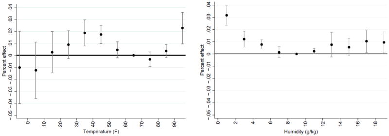
To illustrate my core mortality results, I translate the coefficients in column (3) into percentage changes in the annual mortality rate from exposure to one additional day per year in a given temperature or humidity bin. These estimates, which are presented in Fig. 2, show that one additional day per year between 30 and 40 °F causes the annual mortality rate to increase by approximately 0.02% (relative to 60–70 °F). As Fig. 2 illustrates, the temperature – mortality relationship and the humidity – mortality relationship both are roughly U-shaped. That is, mortality rates decrease as the temperature (humidity) increases until some threshold temperature (humidity) level is reached, after which mortality rates increase as the temperature (humidity) increases. My estimates imply that the ideal temperature and humidity “shocks” are between 70 and 80 °F and between 10 and 12 g/kg, respectively.¹⁰

Fig. 2.

Main results, the percentage change in the annual mortality rate from one additional day within a given temperature or humidity bin relative to 60–70 °F and 8 – 10 g/kg, respectively.

Notes: Regression coefficients from Table 1, column (3), are normalized based on the average mortality rate (per 100,000) for the 373 counties in my sample. The dots represent the point estimates and the brackets represent the 95% confidence interval.

As an aside, Fig. 2 suggests that there may be a positive relationship between mortality and temperature at temperatures below 30 °F, although the parameter estimates are imprecise. The positive relationship is partially due to the fact that motor-vehicle fatalities decrease at colder temperatures.¹¹

6.3. By cause of death

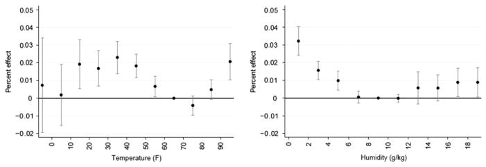
Fig. 3 analyzes the effects of temperature and humidity on two of the most prominent causes of death: cardiovascular disease and cancer.¹² For cardiovascular deaths (Panel A), the temperature – mortality relationship and the humidity – mortality relationship are roughly U-shaped. I find that temperature and humidity have little effect on deaths from cancer (Panel B). Out of 19 parameters in Panel B, only one is statistically significant at conventional levels. Specifically, temperatures above 90 °F have a statistically significant, but economically small, impact on cancer mortalities. Importantly, the near-zero result for cancer-related mortality suggests that my identification strategy has effectively mitigated potential biases from inter-temporal displacement effects since these deaths were already impending and would have occurred in the short-term regardless of the weather [8]. Furthermore, my results are robust to using a three-month moving average (see online Appendix Fig. 1).

Fig. 3.

By primary cause of death, the percentage change in the annual mortality rate from one additional day within a given temperature or humidity bin relative to 60–70°F and 8 – 10 g/kg, respectively. Panel A: Primary cause is cardiovasular and Panel B: Primary cause is cancer.

Notes: See the notes to Fig. 2. Axes vary across Panel A and Panel B.

Fig. 4 examines the effects of temperature and humidity on influenza-related mortalities. Here, I define a death as “influenza-related” when influenza is reported as a primary or secondary cause of death. I use this approach given the primary cause of influenza-related fatalities is frequently listed as cardiovascular disease [17]. My results show a statistically significant and economically meaningful relationship between low-humidity levels and influenza-related fatalities. For example, one additional day with humidity levels between 0 and 2 g/kg causes more than a 1.0% increase in the influenza-related mortality rate. The temperature estimates are generally imprecise at the low end of the temperature distribution, though I find that temperatures between 30 and 50 °F cause a statistically significant increase in influenza-related mortality rates. To my knowledge, this is the first study to demonstrate the relationship between humidity and (human) influenza mortality using a nationally representative sample.¹³ Deeper exploration of this particular result is worthy of study, but must be left for future research.

Fig. 4.

For influenza-related fatalities, the percentage change in the annual mortality rate from one additional day within a given temperature or humidity bin relative to 60–70°F and 8 – 10 g/kg, respectively.

Notes: See the notes to Fig. 2. The standard errors on the coefficient for temperatures below 0 °F and between 10 and 20 °F are too large to be illustrated here. Influenza-related fatalities are defined as any death where influenza is listed as a primary or secondary cause of death.

6.4. Other results and robustness checks

In general, I find a U-shaped temperature – mortality and a U-shaped humidity – mortality relationship across most age groups. However, my estimates are statistically sharper and larger in economic magnitude for people over 45 years of age. Therefore, given the vast majority of deaths are made up of individuals over 45, my core estimates provide an accurate assessment of the aggregate impacts of weather changes. The age-specific estimates are reported in online Appendix Table 1.¹⁴

Appendix Table 1.

Estimates by age groups

Column:	(1)	(2)	(3)	(4)	(5)	(6)	(7)	(8)	(9)	(10)	(11)
Age group:	<1	1–4	5–14	15–24	25–34	35–44	45–54	55–64	65–74	75–84	85+
Mean outcome:	88.6	4.1	2.1	8.0	10.6	19.0	42.8	101.5	229.1	518.1	1280.5
TEMP = <0	−27.7 (16.7)	−0.8 (1.9)	−0.2 (0.8)	−2.5 (1.6)	0.0 (2.0)	0.6 (3.3)	3.5 (3.7)	0.2 (11.8)	14.5 (15.8)	11.1 (31.1)	−8.8 (142.6)
TEMP = 0–10	12.8 (15.0)	−0.7 (1.6)	−0.5 (0.6)	−1.9 (1.2)	0.0 (1.3)	−1.9 (2.0)	4.9 (3.2)	10.2 (6.8)	17.8 (10.3)	4.6 (26.5)	42.7 (66.8)
TEMP = 10–20	−7.3 (9.7)	−0.6 (0.8)	0.3 (0.3)	−1.7 (0.8)	−0.6 (1.1)	−1.3 (1.6)	3.6 (3.1)	4.5 (3.0)	32.8 (7.7)	52.7 (16.1)	139.5 (55.7)
TEMP = 20–30	7.5 (6.9)	−0.5 (0.8)	−0.4 (0.2)	−0.7 (0.6)	−0.2 (0.6)	−1.1 (0.7)	3.0 (1.6)	5.1 (2.6)	19.3 (5.8)	42.0 (12.6)	107.0 (45.8)
TEMP = 30–40	2.7 (5.3)	0.1 (0.6)	0.1 (0.2)	−0.1 (0.4)	0.6 (0.5)	0.3 (0.7)	1.9 (1.2)	3.6 (2.2)	23.3 (5.2)	63.8 (15.7)	166.7 (33.1)
TEMP = 40–50	4.6 (3.5)	0.4 (0.5)	−0.3 (0.2)	0.6 (0.3)	1.0 (0.3)	0.4 (0.5)	1.2 (0.9)	3.7 (1.6)	16.6 (4.0)	40.7 (8.6)	134.4 (26.1)
TEMP = 50–60	1.2 (2.5)	−0.1 (0.4)	−0.1 (0.1)	0.1 (0.2)	0.5 (0.4)	−0.3 (0.4)	0.2 (0.9)	1.3 (1.0)	5.7 (2.0)	22.4 (7.6)	24.2 (20.2)
TEMP = 60–70	--omitted--
TEMP = 70–80	−2.6 (1.9)	−0.3 (0.3)	−0.1 (0.1)	0.1 (0.3)	0.3 (0.3)	−0.8 (0.7)	0.4 (0.8)	−2.1 (1.1)	−1.8 (1.9)	−1.3 (6.6)	−29.6 (18.6)
TEMP = 80–90	−1.9 (3.1)	0.2 (0.3)	0.0 (0.2)	0.3 (0.4)	1.1 (0.5)	1.1 (0.9)	3.2 (1.0)	−0.3 (1.4)	1.2 (3.5)	13.1 (7.2)	4.7 (22.7)
TEMP = 90+	1.0 (6.5)	−0.8 (0.6)	0.7 (0.5)	0.4 (1.0)	1.6 (0.7)	1.5 (1.7)	2.4 (2.9)	7.9 (2.8)	19.9 (6.1)	48.3 (11.2)	113.4 (38.9)
HUMID = 0–2	−2.1 (4.1)	0.9 (0.6)	0.5 (0.2)	−0.5 (0.7)	−0.7 (0.8)	2.2 (1.1)	1.2 (1.5)	7.0 (3.1)	22.1 (3.6)	81.5 (12.3)	334.7 (46.6)
HUMID = 2–4	−5.3 (2.3)	0.3 (0.3)	0.1 (0.1)	−1.0 (0.3)	−0.4 (0.4)	0.0 (0.5)	1.5 (0.9)	4.0 (1.6)	14.2 (3.6)	33.0 (8.5)	199.0 (27.7)
HUMID = 4–6	−6.1 (2.3)	−0.1 (0.3)	0.1 (0.2)	−0.4 (0.2)	−0.5 (0.3)	0.1 (0.5)	0.3 (0.8)	3.3 (1.0)	8.1 (3.7)	23.5 (9.5)	101.8 (29.1)
HUMID = 6–8	−4.4 (2.4)	0.4 (0.3)	0.2 (0.1)	−0.5 (0.3)	−0.3 (0.3)	−1.1 (0.8)	−0.1 (1.1)	0.8 (1.2)	2.7 (1.6)	−6.2 (5.7)	20.5 (12.2)
HUMID = 8–10	--omitted--
HUMID = 10–12	−3.7 (2.6)	0.0 (0.3)	0.1 (0.1)	0.2 (0.2)	0.4 (0.2)	−0.9 (0.4)	−1.0 (0.9)	0.0 (1.1)	0.7 (3.1)	−5.3 (3.8)	−5.8 (11.2)
HUMID = 12–14	4.9 (4.5)	0.4 (0.3)	0.1 (0.2)	0.4 (0.4)	0.5 (0.5)	1.1 (0.8)	−0.3 (1.7)	2.1 (1.6)	5.4 (3.3)	4.1 (4.9)	39.5 (26.8)
HUMID = 14–16	−1.4 (3.5)	0.5 (0.4)	0.3 (0.2)	0.7 (0.6)	0.8 (0.6)	0.1 (1.0)	−0.6 (1.3)	4.9 (1.2)	5.4 (3.1)	7.8 (7.5)	42.2 (19.1)
HUMID = 16–18	6.8 (2.4)	0.4 (0.3)	0.4 (0.1)	0.6 (0.6)	1.2 (0.7)	1.0 (0.7)	−0.1 (1.6)	3.8 (1.4)	8.8 (3.4)	0.8 (5.0)	40.9 (24.6)
HUMID = 18+	9.9 (5.2)	0.7 (0.4)	0.3 (0.3)	0.9 (0.7)	1.4 (0.9)	1.4 (0.8)	1.2 (1.4)	3.2 (2.1)	11.7 (3.5)	0.0 (6.4)	47.9 (33.8)

Notes: This model includes the same controls as the specification in Table 2 column (3). Standard errors in parentheses.

My results are qualitatively similar when I vary the moving average in Eq. (2) to three months (online Appendix Fig. 1). I use a 5th-degree polynomial spline in temperature and humidity (online Appendix Fig. 2). Also, I divide my sample into two sets of counties, “hot” and “cold”, based on the fraction of the year that the temperature is above 65 °F (online Appendix Fig. 3). The temperature – mortality and humidity – mortality relationships both are U-shaped across these hot and cold counties. However, hot counties are less vulnerable to high temperature and high humidity levels compared to cold counties.¹⁵ This result is suggestive that individuals can adapt to climatic differences and reiterates my earlier caveat that the climate-change predictions may represent an upper-bound estimate. However, statistical imprecision precludes making strong conclusions in this regard. Nonetheless, as a robustness check, I use the estimates for the hot counties to make an out-of-sample prediction on the potential impacts of climate change on the full sample of counties.

Appendix Figure 3.

Mortality estimates broken out by hot and cold counties

Panel B: The top 50 percent coldest counties

Notes: See the notes to Figure II. The counties are broken into two mutually exclusive samples based on the fraction of the year with temperatures above 65°F. The standard errors on temperatures below 10°F (Panel A) and temperature above 90°F (Panel B) are too large to be displayed here.

I estimate a state-month model, where the controls are identical to Eq. (2) except at the state-level (online Appendix Fig. 4). Recall that due to data constraints in the MCOD files, I only have identifiers for counties with over 100,000 inhabitants. With the state-month model, I can include almost all deaths reported in the MCOD files.¹⁶ Both models produce nearly identical estimates. The only meaningful difference is that the estimated effects of temperatures above 90 °F are larger in magnitude in the state model; this suggests that my core model might slightly underestimate the adverse effects of climate change.

In robustness checks not reported, I estimate a model using diurnal temperatures, since there is the possibility that humidity is a proxy for diurnal temperature. In this specification, I find slightly larger impacts on mortality rates at temperatures above 90 °F, but nearly identical estimates on my humidity parameters. Heat waves, or three consecutive days with daily mean temperatures above 90 °F, cause a small but statistically insignificant increase in the mortality rate. I examine the sensitivity of my results to varying the set of fixed effects by replacing the county by calendar month quadratic trends with linear trends. (Results available upon request.)

7. Results: the effects of temperature and humidity on energy consumption

In order to evaluate potential adaptation mechanisms, I explore the responsiveness of energy consumption to changes in temperature and humidity. Specifically, I estimate the effects of temperature and humidity on per capita energy consumption in the residential sector using data from the Energy Information Administration (EIA) [24]. The EIA reports total energy consumption in British Thermal Units (BTU) for the residential sector by state and year from 1960 to the present.

I restrict my sample to 1973–2002 due to the data quality issues in the GSOD data mentioned above. I create per capita energy consumption data using population estimates provided by the EIA. Following DG, I focus on the residential sector because the responsiveness of energy consumption to weather is likely to be greater than in other sectors.

The unit of observation in the EIA data is at the state-year level; so I must rely on a model different from Eq. (1). Specifically, I estimate the following reduced-form model:

$$C_{ky}=\sum _b{\beta }^b{\mathit{TEMP}}_{ky}^b+{\sum }_{b^{\prime }}{\propto }^{b^{\prime }}{\mathit{HUMID}}_{ky}^{b^{\prime }}+X_{ky}\gamma +{\mu }_y+{\delta }_k\mathit{YEAR}+{\pi }_k{\mathit{YEAR}}^2+e_{\mathit{kym}}$$ (3)

where C is the per capita energy consumption in the residential sector in state k and year y; the weather variables are as in Eq. (2) except my sample of county-month weather data are aggregated to the state-year level using the county’s population in 2000 as weights (U.S. Census Bureau [31]); year fixed effects (μ) control for macro-level shocks; and state-specific quadratic time trends (YEAR and YEAR²) are included to account for the possibility that trends in energy consumption are spuriously correlated with state-specific climatic trends.

My energy estimates, which are presented in Fig. 5, show a roughly U-shaped temperature – energy consumption relationship. For example, one additional day per year with temperatures between 20 and 30 °F causes annual per capita energy consumption in the residential sector to increase by 0.3% (relative to 60–70 °F). One additional day per year with temperatures above 90 °F causes energy consumption to increase by 0.2%.

Fig. 5.

The percentage change in annual per capita energy consumption in the residential sector from one additional day within a given temperature or humidity bin relative to 60–70 °F and 8 – 10 g/kg, respectively.

Notes: See notes to Fig. 2. Regression estimates were normalized based on average energy consumption over the 1973–2002 period.

Energy consumption increases only slightly with increases in humidity levels. For example, one additional day per year with humidity levels above 18 g/kg causes annual energy consumption to increase by about 0.02% (relative to 8 – 10 g/kg), which is about a tenth of the effect size on temperatures above 90 °F. One additional day per year with humidity levels between 0 and 2 g/kg has no discernable effect on energy consumption. Moreover, only one of the nine humidity parameters (i.e., 14–16 g/kg) is statistically significant at conventional levels.

The unresponsiveness of energy consumption to changes in humidity can potentially be explained by the fact that relatively few households in the United States own humidifiers and dehumidifiers. According to the EIA, approximately 15% of all households had humidifiers and 11% had dehumidifiers in 2001 [18]. Conversely, approximately 76% of all households possessed air conditioners [18]. The small increase in energy consumption at high-humidity levels may be due to the increased use of air conditioners, since temperature reductions can actually offset the heat stress induced by high temperature – humidity combinations [19].

As an important aside, the fact that energy consumption is unresponsive to low-humidity levels, in particular, may have important implications for public-health policy. According to my core mortality estimates (Fig. 2), humidity levels below 6 g/kg cause a large increase in mortality rates. However, there is little apparent self-protection, in the form of increased energy consumption from these dangerous humidity levels. To the extent that existing technologies (e.g. humidifiers) can mitigate the adverse health effects of low-humidity levels, then policy intervention may have significant economic returns. However, I cannot definitively identify the particular mechanism through which low-humidity levels impact mortality since, for one, I cannot distinguish outdoor from indoor exposure. More research is necessary to determine the optimal form of intervention.

8. Climate change projections

8.1. Welfare valuations

The A1F1 scenario of the Hadley CM3 model predicts significantly more hot and humid weather by the end of the 21st century. Fig. 6 illustrates both the “bias-corrected” and “uncorrected” differences in the daily temperature and daily humidity distributions between the GSOD sample period (c. 1973–2002) and the Hadley CM3 end-of-century predictions (c. 2070–2099). Focusing on the bias-corrected predictions for the moment, the Hadley CM3 model predicts that the United States will experience approximately 10 fewer days between 30 and 40 °F and almost 40 more days over 90 °F per year on average by the end of the 21st century, and there will be approximately 20 fewer days with humidity levels below 2 g/kg and about 35 more days with humidity levels above 18 g/kg per year on average.

Fig. 6.

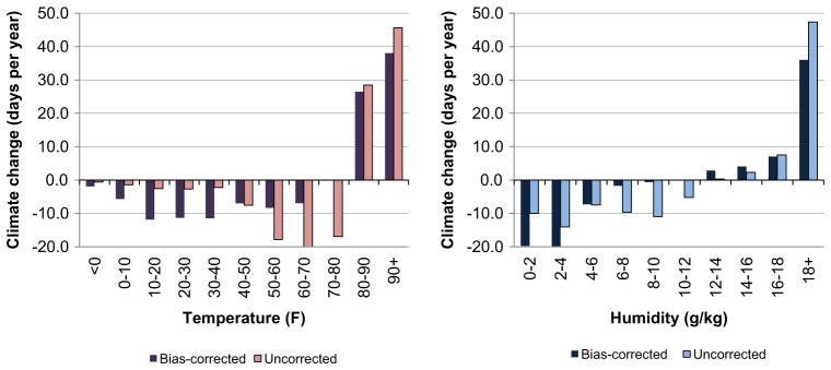
Climatic changes (in days per year) between the 1973–2002 period and the 2070–2099 period, A1F1 scenario of the Hadley CM3 climate-change model.

Notes: The bias-corrected predictions adjust for differences between the Hadley CM3 model data and the GSOD weather data between 1990 and 2002. The predicted climatic changes only pertain to the 373 counties in my core sample.

The uncorrected predictions present a qualitatively similar picture, but with slightly more hot and humid weather. For example, the uncorrected Hadley CM3 model predicts some 45 more days with temperatures above 90 °F and nearly 50 more days with humidity levels above 18 g/kg. The differences between the bias-corrected and uncorrected predications indicate that the United States realized generally milder weather conditions between 1990 and 2002 than predicted by the Hadley CM3 climate model. Therefore, the bias-corrected predictions show that climate change will have a more favorable impact on mortality.

Coupled with my core temperature – mortality and humidity – mortality model and the uncorrected Hadley CM3 predictions, I project that mortality rates are likely to decrease by approximately 0.08%, or two thousand fewer deaths, by the end of the 21st century (c. 2070–2099).¹⁷ Using my age-specific estimates (online Appendix Table 1) and life expectancy estimates for the year 2000 from the Center for Disease Control and Prevention [20], I find that each additional death is associated with around 25 years of lost life on average.¹⁸ Assuming a statistical value of a one year of life is $100,000 (as done by DG and others), my estimates imply that climate change will benefit the United States by a negligible $5 billion dollars in terms of saved lives. The projected decrease in mortality rates is not statistically significant from zero at conventional levels. Compared to DG, I estimate that climate change will have a more favorable impact on mortality rates. The difference between DG’s projections and my own can potentially be explained by the fact that I rely on the subset of counties with over 100,000 inhabitants.¹⁹

Furthermore, I project that there will be a 3.5% decrease in energy consumption in the residential sector. (Or, a decrease of 7.1 quadrillion BTUs.) Assuming a price per quadrillion BTU of $7.6 million (in 2006$), as done by DG, this translates into $54 billion less in energy expenditures per year. However, my energy projection is not statistically significant from zero at conventional levels. Compared to DG, I also estimate a more favorable impact of climate change on energy consumption. My energy predictions, along with various robustness checks, are available in online Appendix Table 2.

Appendix Table 2.

Projected percentage change in energy consumption by 2070–2099, bias-corrected Hadley CM3 (A1F1) climate model

Model:	(1)	(2)	(3)	(4)	(5)	(6)	(7)
	Core model	No humidity controls	Add diurnal temperatures	Add relative humidity	Add “heat waves” controls	5th degree spline	Uncorrected Hadley CM3
Entire United States	−3.5 (1.9)	−4.4 (1.7)	−3.4 (2.2)	−2.5 (2.2)	−3.7 (3.1)	−1.8 (2.4)	5.4 (3.0)
New England	−9.2 (1.4)	−9.5 (1.4)	−9.5 (1.5)	−8.3 (1.5)	−9.3 (1.7)	−10.4 (1.6)	−4.2 (2.2)
Middle Atlantic	−9.0 (1.8)	−9.5 (1.7)	−9.0 (2.0)	−7.7 (2.1)	−9.1 (2.3)	−9.8 (2.1)	0.8 (2.8)
East North Central	−7.5 (1.7)	−8.2 (1.5)	−7.2 (2.0)	−6.6 (2.0)	−7.7 (2.5)	−6.4 (1.8)	−0.6 (2.7)
West North Central	−6.2 (2.1)	−7.2 (1.8)	−4.8 (2.8)	−5.3 (2.6)	−6.4 (3.4)	−2.4 (2.5)	2.7 (3.1)
South Atlantic	5.8 (2.4)	4.7 (1.9)	7.9 (2.4)	8.0 (2.9)	5.6 (3.9)	4.5 (5.7)	9.3 (4.2)
East South Central	1.7 (2.4)	0.3 (2.1)	3.2 (2.7)	2.9 (2.8)	1.5 (4.2)	5.7 (2.8)	9.3 (3.7)
West South Central	6.4 (3.3)	4.5 (2.8)	9.6 (4.4)	7.5 (3.7)	6.0 (6.0)	15.3 (3.9)	13.7 (4.8)
Mountain	−5.6 (1.9)	−6.4 (1.7)	−6.0 (2.3)	−5.4 (2.2)	−5.7 (3.1)	−3.3 (2.2)	4.9 (2.3)
Pacific	−4.9 (2.2)	−6.1 (2.1)	−8.8 (2.9)	−4.9 (2.3)	−5.1 (3.5)	−1.5 (2.2)	12.5 (2.7)

Notes: Standard errors in parentheses.

Together, the health-related savings of climate change (in terms of mortality and energy consumption) is $58 billion dollars per year. Put another way, this translates into savings of about $195 per capita per year ($58 billion divided by 300 million people). This is a tiny amount relative to the United States’ baseline income per capita of around $35 thousand [21].

Using the uncorrected Hadley CM3 predictions, I project a 1.0% increase in mortality rates and a 5.4% increase in energy consumption by the end of the 20th century. The welfare cost, with the uncorrected climate predictions, totals $142 billion dollars per year ($474 per capita). Neither my mortality projections nor my energy projections are statistically different from zero at conventional levels using the uncorrected climate predictions. Nonetheless, this exercise suggests that under a different, and possibly very realistic, climate-change scenario, the aggregate impacts on mortality and energy consumption will be moderately worse than predicted by the bias-corrected model.

On the whole, my projections, both with the bias-corrected and uncorrected Hadley CM3 predictions, suggest that climate change will have a small impact on aggregate mortality rates in the United States in the coming century. However, the distributional impacts of climate change are meaningful. The bias-corrected predictions imply 1.9%, 1.2%, and 2.9% increases in mortality rates in South Atlantic, East South Central, and West South Central Divisions, respectively. Using the uncorrected climate-change predictions, I project that these three southern divisions will experience a 2.3%, 2.4%, and 4.7% increase in mortality rates (see Table 3). Conversely, the Northern Divisions will mostly see a decline in mortality rates. For example, the New England Division is predicted to experience a 1.1% decrease and a 1.3% decrease in mortality rates under the bias-corrected and uncorrected climate change scenarios, respectively. Therefore, the aggregate estimates obfuscate the fact that the costs of climate change are going to be borne disproportionately by the south, which is relatively poorer than the rest of the country [22].

Table 3.

Projected percentage change in mortality rates (c. 2070–2099) using the Hadley CM3 (A1F1) model.

Division	Bias-corrected Hadley CM3			Uncorrected Hadley CM3
	(1) Core model	(2) No humidity controls	(1)–(2) Difference	(4) Core model	(5) No humidity controls	(4)–(5) Difference
Entire United States	−0.08 (0.62)	−0.94 (0.42)	0.86 (0.32)	0.98 (0.60)	0.48 (0.34)	0.50 (0.35)
New England	−1.08 (0.53)	−1.69 (0.41)	0.61 (0.18)	−1.29 (0.51)	−1.07 (0.35)	−0.21 (0.20)
Middle Atlantic	−0.66 (0.53)	−1.41 (0.39)	0.75 (0.21)	−0.36 (0.47)	−0.32 (0.28)	−0.03 (0.24)
East North Central	−0.36 (0.57)	−1.16 (0.38)	0.80 (0.29)	−0.08 (0.60)	−0.25 (0.36)	0.17 (0.32)
West North Central	0.44 (0.70)	−0.77 (0.40)	1.21 (0.43)	0.91 (0.83)	0.38 (0.44)	0.54 (0.51)
South Atlantic	1.91 (0.85)	0.11 (0.40)	1.80 (0.61)	2.29 (0.90)	0.68 (0.35)	1.62 (0.68)
East South Central	1.23 (0.81)	−0.29 (0.40)	1.52 (0.56)	2.44 (0.95)	1.06 (0.38)	1.38 (0.68)
West South Central	2.92 (1.35)	0.37 (0.58)	2.55 (1.00)	4.68 (1.69)	2.10 (0.66)	2.58 (1.25)
Mountain	−1.85 (0.52)	−1.42 (0.46)	−0.43 (0.11)	−0.04 (0.20)	1.06 (0.15)	−1.11 (0.24)
Pacific	−1.96 (0.55)	−1.54 (0.51)	−0.43 (0.10)	1.50 (0.36)	1.55 (0.39)	−0.06 (0.13)

Notes: Standard errors are in parentheses. The bias-corrected predictions adjust for differences in the actual weather data and the Hadley CM3 model predictions between 1990 and 2002. The projections only pertain to the 373 counties used in my core analyses.

8.2. Discussion: importance of controlling for humidity

On the aggregate, excluding humidity makes me to underestimate the costs (or overstate the benefits) of climate change by a small amount. As Table 3 illustrates, I estimate a 0.94% decrease in mortality rates when I fail to control for humidity (column 2), as opposed to a 0.08% decrease in mortality in my core model (column 1). The difference, which is statistically significant at conventional levels, is only somewhat economically meaningful: omitting humidity underestimates the mortality costs of climate change by about $53 billion.²⁰

However, incorporating humidity is particularly important in the context of evaluating the distributional impacts of climate change. As column (2) indicates, omitting humidity leads me to noticeably underestimate the mortality costs of climate change in the South. For example, the West South Central Division (where Louisiana is located, for one) is expected to see a 2.9% increase in mortality rates with my core model (column 1), but only a 0.4% increase when neglecting to control for humidity. Conversely, the Middle Atlantic Division (where New York is located) has 0.7% decline in mortality rates in my core model, but a 1.4% decline in mortality without controlling for humidity. Importantly, the difference is statistically significant in all the nine divisions (column 3).

Controlling for humidity is similarly important when I use the uncorrected climate-change predications. That is, omitting humidity leads me to overstate the mortality benefits by 0.5% points for the entire United States (column 6). Also, omitting humidity leads me to underestimate the mortality impacts of climate change by 1.6%, 1.4%, and 2.6% points in the South Atlantic, East South Central, and West South Central Divisions, respectively. With the uncorrected projections, the differences between the two models are statistically significant in four of the nine divisions.

A fundamental contribution of my work is to demonstrate that accounting for humidity is particularly important when evaluating the distributional effects of climate-change. My results suggest that omitting humidity underestimates the extent to which the poor will be impacted by climate change. Therefore, accounting for humidity has important implications for devising equitable climate-change policies. As an aside, controlling for humidity is apt to be even more important when projecting the impacts of climate change across countries since climatic differences, with regards to humidity, are much greater.

8.3. Robustness checks

Table 4 presents a variety of robustness checks. Specifically, I drop the temperature – humidity interaction terms (column 1). I add controls for 10 °F-binned diurnal temperatures (column 2), relative humidity (column 3), and “heat waves” (column 4).²¹ I use a three-month moving average when constructing the weather variables (column 5). I control for county-by-month linear trends in place of the quadratic trends (column 6). I use a 5th-degree cubic spline to model the weather variables (column 7). I project the effects of climate change on the full sample of counties using the estimates from the sample of hot counties (column 8). In general, my mortality projections, both across divisions and on aggregate, are robust to these modifications. The most notable result from Table 4 is that my projections are slightly more modest when I drop the temperature – humidity interaction terms.

Table 4.

Projected percentage change in mortality rates (c. 2070–2099) using bias-corrected Hadley CM3 model, robustness checks.

Model	(1) No humidity interaction terms	(2) Add diurnal temperatures	(3) Add relative humidity	(4) Add “heat waves” controls	(5) 3-month moving average	(6) Linear time trends only	(7) Cubic spline	(8) Using estimates from hot counties
Entire United States	−0.64 (0.49)	−0.10 (0.64)	−0.48 (0.65)	−0.18 (0.55)	0.39 (0.77)	−0.35 (0.60)	−0.25 (0.60)	−0.98 (0.70)
New England	−1.34 (0.49)	−1.21 (0.53)	−1.27 (0.54)	−1.12 (0.49)	−0.38 (0.64)	−1.27 (0.62)	−1.20 (0.54)	−1.97 (0.66)
Middle Atlantic	−1.02 (0.47)	−0.72 (0.54)	−0.90 (0.56)	−0.71 (0.48)	−0.05 (0.65)	−0.88 (0.58)	−0.82 (0.53)	−1.53 (0.64)
East North Central	−0.84 (0.45)	−0.35 (0.59)	−0.76 (0.61)	−0.45 (0.49)	0.33 (0.71)	−0.55 (0.54)	−0.53 (0.52)	−1.05 (0.67)
West North Central	−0.32 (0.46)	0.47 (0.75)	−0.17 (0.77)	0.30 (0.63)	1.09 (0.86)	0.20 (0.59)	0.25 (0.59)	−0.02 (0.74)
South Atlantic	0.57 (0.49)	1.85 (0.87)	1.02 (0.91)	1.79 (0.80)	1.76 (1.01)	1.29 (0.69)	1.52 (0.78)	0.77 (0.80)
East South Central	0.16 (0.47)	1.24 (0.86)	0.50 (0.86)	1.09 (0.75)	1.33 (0.99)	0.82 (0.63)	1.05 (0.67)	0.25 (0.80)
West South Central	1.03 (0.68)	3.02 (1.47)	1.65 (1.41)	2.69 (1.27)	2.77 (1.60)	2.27 (0.99)	2.67 (1.06)	1.51 (1.25)
Mountain	−1.63 (0.52)	−1.86 (0.53)	−1.73 (0.54)	−1.96 (0.44)	−0.92 (0.71)	−1.86 (0.54)	−1.87 (0.54)	−2.71 (0.68)
Pacific	−1.64 (0.55)	−1.94 (0.60)	−1.77 (0.54)	−2.07 (0.52)	−1.20 (0.71)	−1.93 (0.60)	−1.93 (0.57)	−2.76 (0.81)

Notes: Standard errors in parentheses. See text for more discussion on the particulars of each of these different models. The projections only pertain to the 373 counties used in my core analyses.

9. Conclusions

My research explores the impacts of temperature and humidity on some of the health-related costs of climate change for the United States. To my knowledge, this is the first study to provide comprehensive evidence that humidity, like temperature, is an important determinant of mortality. Under a “business-as-usual” climate-change scenario, I project that mortality rates will change very little on the aggregate for the United States by the end of the 21st century. However, the distributional impacts are meaningful: cold and dry areas will benefit from climate change (e.g. the North), while hot and humid areas (e.g. the South) will be worse off.

Moreover, controlling for humidity is particularly important in the context of predicting the distributional effects of climate change. Specifically, neglecting to control for humidity causes me to underestimate the costs of climate change in hot and humid areas, like the South. Given poverty rates are highest in hot and humid areas both within the United States and around the world, properly accounting for humidity has important implications for devising optimal climate-change policies that address concerns of fairness and equity.

Finally, my work offers an important public-health lesson: low-humidity levels cause a large increase in mortality rates, potentially via influenza-related mechanisms. However, there appears to be little self-protection with respect to low-humidity levels based on the empirical fact that energy consumption responds little to changes in humidity. Given the lack of previous research on the humidity – mortality relationship, one plausible explanation is that individuals may be unaware of the dangers of low-humidity levels. This possibility underscores the importance of my work here. Future research should evaluate whether public-health interventions can help mitigate the health impacts of low-humidity levels.

References

- 1.Deschênes Olivier, Greenstone Michael DG. Working Paper no. 13178. June. NBER; Cambridge, MA: 2007. Climate Change, Mortality and Adaptation: Evidence from Annual Fluctuations in Weather in the United States. [Google Scholar]
- 2.Gaffen Dian J, Ross Rebecca J. Climatology and trends of United States surface humidity and temperature. Journal of Climate. 1999;12:811–828. [Google Scholar]
- 3.Willett Katherine M, Gillett Nathan P, Jones Philip D, Thorne Peter W. Attribution of observed surface humidity changes to human influence. Nature. 2007;449:710–713. doi: 10.1038/nature06207. [DOI] [PubMed] [Google Scholar]
- 4.Allali Abdelkader, Bojariu Roxana, Diaz Sandra, Elgizouli Ismail, Griggs Dave, Hawkins David, Hohmeyer Olav, editors. International Panel on Climate Change (IPCC) Climate Change 2007: Synthesis Report. Cambridge University Press; Cambridge, UK and New York, NY, USA: 2007. [Google Scholar]
- 5.Schwartz Joel, Samet Jonathan M, Patz Jonathan A. Hospital admissions for heart disease. the effects of temperature and humidity. Epidemiology. 2004;15:755–761. doi: 10.1097/01.ede.0000134875.15919.0f. [DOI] [PubMed] [Google Scholar]
- 6.Braga Alfesio LF, Zanobetti Antonella, Schwartz Joel. The effect of weather on respiratory and cardiovascular deaths in 12 United States cities. Environmental Health Perspectives. 2002;110(9):859–863. doi: 10.1289/ehp.02110859. [DOI] [PMC free article] [PubMed] [Google Scholar]
- 7.Martens WJM. Climate change, thermal stress and mortality changes. Social Science and Medicine. 1998;46(3):331–344. doi: 10.1016/s0277-9536(97)00162-7. [DOI] [PubMed] [Google Scholar]
- 8.Deschênes Olivier, Moretti Enrico. Working Paper no. 13227. July. NBER; Cambridge, MA: 2007. Extreme Weather Events, Mortality and Migration. [Google Scholar]
- 9.Lowen Anice C, Mubareka Samira, Steel John, Palese Peter. Influenza virus transmission is dependent on relative humidity and temperature. PLoS Pathegen. 2007;3(10):1470–1476. doi: 10.1371/journal.ppat.0030151. [DOI] [PMC free article] [PubMed] [Google Scholar]
- 10.Shaman Jeffrey, Kohn Melvin. Absolute humidity modulates influenza survival, transmission, and seasonality. PNAS. 2009;106(9):3243–3248. doi: 10.1073/pnas.0806852106. [DOI] [PMC free article] [PubMed] [Google Scholar]
- 11.Xie X, Li Y, Chwang ATY, Ho PL, Seto WH. How far droplets can move in indoor environments—revisiting the Wells evaporation-falling curve. Indoor Air. 2007;17:211–225. doi: 10.1111/j.1600-0668.2007.00469.x. [DOI] [PubMed] [Google Scholar]
- 12.Ahrens Donald C. Meteorology Today. 9. Brooks/Cole; St. Paul, MN: 2009. [Google Scholar]
- 13.Baughman Anne V, Arens Edward A. Indoor humidity and human health—part i: literature review of humidity-influenced indoor pollutants. ASHRAE Transactions Research. 1996;102(1):193–211. [Google Scholar]
- 14.Schlenker Wolfram, Roberts Michael. Working Paper no. 13799. February. NBER; Cambridge, MA: 2008. Estimating the Impact of Climate Change on Crop Yields: the Importance of Nonlinear Temperature Effects. [Google Scholar]
- 15.Stern Nicholas. The economics of climate change. American Economic Review: Papers & Proceedings. 2008;98:1–37. [Google Scholar]
- 16.Eisenberg Daniel, Warner Kenneth E. Effects of snowfalls on motor vehicle collisions, injuries, and fatalities. American Journal of Public Health. 2005;95(1):120–124. doi: 10.2105/AJPH.2004.048926. [DOI] [PMC free article] [PubMed] [Google Scholar]
- 17.Madjid Mohammad, Aboshady Ibrahim, Awan Imran, Litovsky Silvio, Ward Casscells S. Influenza and cardiovascular disease. Is there a causal relationship? Teax Heart Institute. 2004;31(1):4–13. [PMC free article] [PubMed] [Google Scholar]
- 18.Energy Information Administration (EIA) Electricity Consumption by End Use in US Households. 2001 Downloaded April, 2009 from < www.eia.doe.gov/emeu/reps/enduse/er01_us_Table1.html>.
- 19.Steadman Robert G. The assessment of sultriness. Part I: a temperature – humidity index based on human physiology and clothing science. Journal of Applied Meteorology. 1979;18:861–873. [Google Scholar]
- 20.Center for Disease Control and Prevention. [accessed January 2010];United States Life Tables. 1999–2003 Downloaded from < http://www.cdc.gov/nchs/nvss/mortality/lewk3.htm>.
- 21.Bureau of Economic Analysis (BEA) Regional Economic Accounts. U.S. Department of Commerce; Downloaded June, 2009 from < http://www.bea.gov/regional/gsp/>. [Google Scholar]
- 22.U.S. Census Bureau. Percent in Poverty. 2007 Downloaded July 2009 from: < http://www.census.gov/did/www/saipe/data/statecounty/maps/iy2007/Tot_Pct_Poor2007.pdf>.
- 23.British Atmospheric Data Centre (BADC) Hadley Centre CM3 Model (A1F1 Scenario) Downloaded May, 2009 from < http://badc.nerc.ac.uk/home>.
- 24.Energy Information Administration (EIA) State Energy Consumption Data. Downloaded November 2008 from < http://www.eia.doe.gov/emeu/states/_seds_tech_notes.html>.
- 25.Hanigan Ivan, Hall Gillian, Dear Keith BG. A comparison of methods for calculating population exposure estimates of daily weather for health research. International Journal of Health Geographics. 2006;5:38. doi: 10.1186/1476-072X-5-38. [DOI] [PMC free article] [PubMed] [Google Scholar]
- 26.National Cancer Institute. US Population Estimates 1968 – 2005. Downloaded March 2008 from < http://seer.cancer.gov/popdata/download.html>.
- 27.National Center for Health Statistics. Multiple Causes of Death Files: 1968–2002. Downloaded March 2008 from the NBER website < http://www.nber.org/data/vital-statistics-mortality-data-multiple-cause-of-death.html>.
- 28.National Climatic Data Center. Global Summary of the Day Files: 1967–2002. Downloaded March 2008 from < ftp://ftp.ncdc.noaa.gov/pub/data/gsod/>.
- 29.Rising Bill. Statistical Software Components S372502. Boston College Department of Economics; SPHDIST: stata module to compute spherical distances. revised 19 June 2000. [Google Scholar]
- 31.U.S. Census Bureau. Census 2000 United States Gazetteer Files. Downloaded March 2008 from < http://www.census.gov/geo/www/gazetteer/places2k.html>.