Functional specialization in rat occipital and temporal visual cortex

Ben Vermaercke; Florian J Gerich; Ellen Ytebrouck; Lutgarde Arckens; Hans P Op de Beeck; Gert Van den Bergh

doi:10.1152/jn.00737.2013

. 2014 Jul 2;112(8):1963–1983. doi: 10.1152/jn.00737.2013

Functional specialization in rat occipital and temporal visual cortex

Ben Vermaercke ¹, Florian J Gerich ¹, Ellen Ytebrouck ², Lutgarde Arckens ², Hans P Op de Beeck ^1,^✉, Gert Van den Bergh ¹

PMCID: PMC4200005 PMID: 24990566

Abstract

Recent studies have revealed a surprising degree of functional specialization in rodent visual cortex. Anatomically, suggestions have been made about the existence of hierarchical pathways with similarities to the ventral and dorsal pathways in primates. Here we aimed to characterize some important functional properties in part of the supposed “ventral” pathway in rats. We investigated the functional properties along a progression of five visual areas in awake rats, from primary visual cortex (V1) over lateromedial (LM), latero-intermediate (LI), and laterolateral (LL) areas up to the newly found lateral occipito-temporal cortex (TO). Response latency increased >20 ms from areas V1/LM/LI to areas LL and TO. Orientation and direction selectivity for the used grating patterns increased gradually from V1 to TO. Overall responsiveness and selectivity to shape stimuli decreased from V1 to TO and was increasingly dependent upon shape motion. Neural similarity for shapes could be accounted for by a simple computational model in V1, but not in the other areas. Across areas, we find a gradual change in which stimulus pairs are most discriminable. Finally, tolerance to position changes increased toward TO. These findings provide unique information about possible commonalities and differences between rodents and primates in hierarchical cortical processing.

Keywords: high-level vision, population coding, position tolerance, rodent research, single-unit recordings

monkeys have been the preferred animal model for vision. Studies have defined more than 30 separate visual areas with many functional differences (Felleman and Van Essen 1991). These areas are organized in a hierarchical way, so that information that enters cortex in primary visual cortex (V1) is processed in multiple steps. Multiple hierarchical streams exist, such as the ventral pathway, important for object recognition, and the dorsal pathway, critical for the link between perception and action (Goodale and Milner 1992; Mishkin and Ungerleider 1982). Along each pathway, response properties change gradually. For example, in the ventral pathway a gradual increase in the tolerance for image transformations occurs together with the emergence of complex selectivity (for review, see Dicarlo et al. 2012). The resulting representations are perfectly fit for, e.g., recognizing a face irrespective of its position and size.

Recently, more and more studies have started to use rodents (mainly mice and rats) as an alternative animal model. Research into the cellular and molecular underpinnings of high-level vision would benefit significantly if rodents turn out to display at least a rudimentary version of the pathways defined in primates. However, functional evidence for a multistep cortical hierarchy is limited. Recent studies focusing upon functional organization in rodent visual cortex (Andermann et al. 2011; Marshel et al. 2011; Wang et al. 2012) mostly provide evidence for a two-step system, V1 plus one step. Anatomically, most visual regions form a ring around V1 and are thus adjacent to V1, and all known regions in mice receive substantial input directly from V1. Although other anatomical criteria have suggested the existence of hierarchical pathways in rodents (for anatomical evidence, see Wang and Burkhalter 2007; Wang et al. 2012), including a ventral pathway extending laterally into the temporal lobe, functional evidence for any hierarchy among the extrastriate regions is scarce.

In addition, studies of extrastriate regions in rodents were motivated by how V1 is studied, using similar stimuli (e.g., moving gratings) and describing the tuning in terms of simple parameters. Such stimuli and parameters would not reveal any high-level processing, a term that is typically used in primate studies on, e.g., the ventral object vision pathway. “High-level” vision is typically studied with two types of stimuli: either by building stimulus complexity using combinations of simple features or by using more complex arbitrary shapes. Here we took the second approach, performing experiments with a type of shape stimuli that has been used in primates before (Lehky and Sereno 2007).

In the present study we targeted V1 and the most temporal extrastriate areas described previously in rat [lateromedial (LM), latero-intermediate (LI), and laterolateral (LL); see Espinoza and Thomas 1983; Montero 1993; Olavarria and Montero 1984; Thomas and Espinoza 1987] and found evidence for a progression of not four but even five areas. We measured the functional properties of neurons with extracellular single-unit recordings in all five areas in awake rats. Along this recording trajectory, we observed changes in functional properties that are consistent with the object vision pathway in primates in some aspects (e.g., increase in position tolerance), but without the strict segregation of form and motion and without the strong bias to process more complex stimuli than gratings.

MATERIALS AND METHODS

Animal Preparation, Surgery, and Habituation

All experiments and procedures involving living animals were approved by the Ethical Committee of the University of Leuven and were in accordance with the European Commission Directive of September 22nd 2010 (2010/63/EU). We performed microelectrode recordings in awake hybrid Fischer/Brown Norway F1 rats (n = 8 males), obtained from Harlan Laboratories (Indianapolis, IN). Rats aged between 3 and 12 mo were anesthetized with ketamine-xylazine. Six rats received a stereotaxically positioned 2-mm-diameter circular craniotomy at −7.90 mm posterior and 3.45 mm lateral from bregma. A metal recording chamber with a base angle of 45° was placed on top of the craniotomy. Two rats received a vertical recording chamber positioned for orthogonal cortical penetrations in V1. A triangular headpost was fitted on top of bregma. A CT scan of the head confirmed the position of the recording chamber and craniotomy (Fig. 1A). To alleviate pain, buprenorphine (50 μg/kg ip) was administered postoperatively every 24 h for up to 3 days.

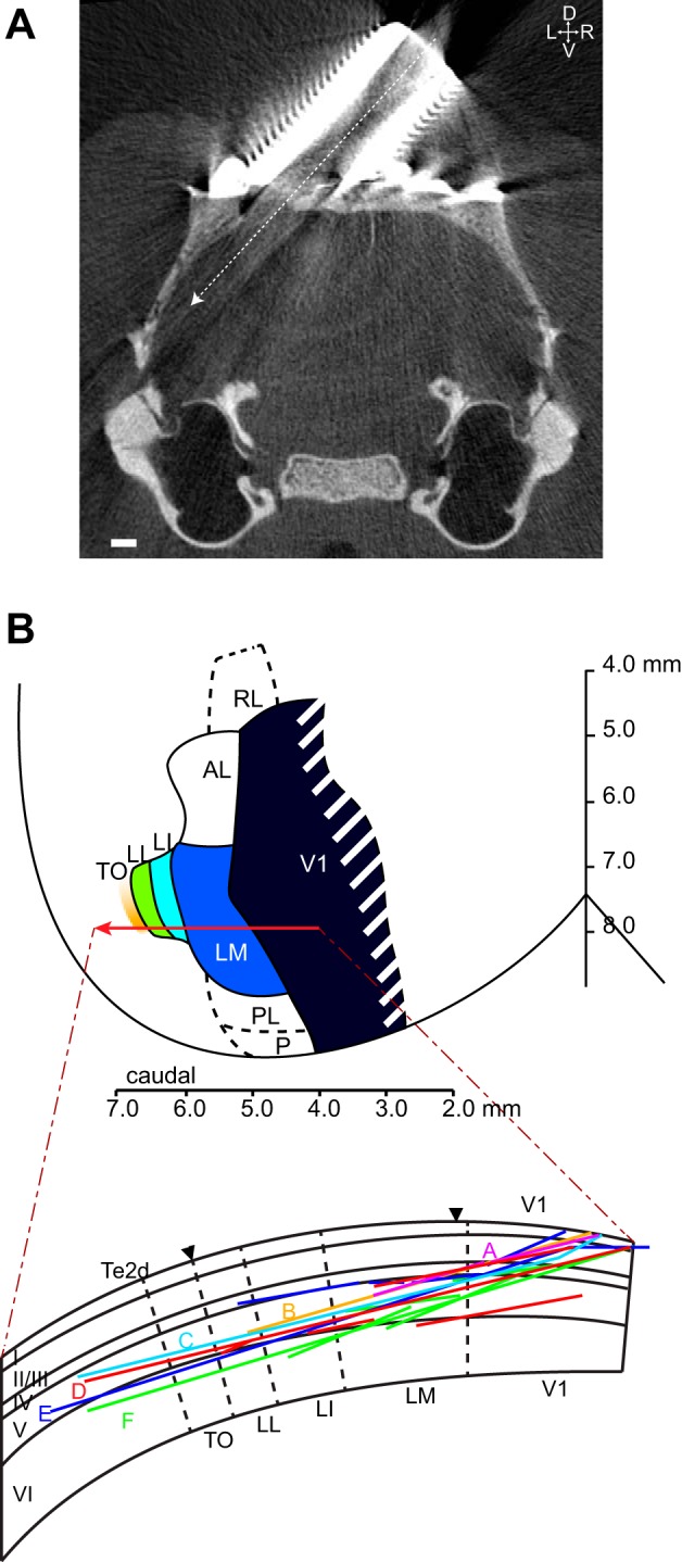
Fig. 1. — Localization of electrode tracks. A: representative coronal section of a CT scan of rat skull at the location of the craniotomy and recording chamber implant (7.9 mm caudal from bregma), showing the position of the craniotomy and the predicted electrode track. Scale bar, 1 mm. B, *top*: schematic overview of V1 and lateral extrastriate regions in the rat, based on the electrophysiological maps of Espinoza and Thomas (1983) and Thomas and Espinoza (1987). Red arrow represents the schematic anteroposterior location of our electrode tracks in relation to the different extrastriate areas: lateromedial (LM), latero-intermediate (LI), laterolateral (LL), and lateral occipito-temporal cortex (TO). *Bottom*: schematic overview of the relative position of the different electrode tracks (as derived from histology) within our 6 animals (*animals A–F*; each animal is differently colored) plotted on a schematic coronal slice (see Fig. 3B), indicating depth distribution of our tracks within the visual cortex. Note that many penetrations were performed in the animals, much more than the number of tracks that can be individuated from histology (most likely because most penetrations fall along the same line, as intended by the experimenter).

We habituated the animal to be head restrained by gradually increasing the time it was head fixed in the setup in daily sessions from 8 min to 2 h and 30 min, over 2 wk. During head restraint, the headpost was fixed by a custom-built metal arm that left the right visual field unrestricted. Except for its head, the animal was completely surrounded by a wooden box, to limit body movements. Rats were water deprived so that water was only provided to the animal during head restraint or immediately after training. During electrophysiological recording sessions, a drop of water was given every tenth visual stimulus. This procedure limited the amount of body movement of the rats during experiments and increased their attention as they remained focused on receiving water rewards.

When the animal was able to be head restrained for at least 1 h and 30 min, we started with our recording sessions. A recording session generally lasted between 2 and 3 h. After removal of the electrode, cleaning, and capping of the recording chamber, the animal was released from the head holder and rewarded with water in its home cage.

Electrophysiological Recordings

A Biela Microdrive (Crist Instruments, Hagerstown, MD) containing a 5- to 10-MΩ-impedance tungsten electrode (FHC, Bowdoin, ME) was placed on the recording chamber. The electrode was manually moved into the brain at an angle of 45° (AP: −7.9 mm; ML: 3.5 mm) in steps of at most 100 μm (a quarter turn of the Biela drive, full turn = 385 μm), thereby entering five different consecutive visual areas: V1, LM, LI, LL, and TO. In each animal, we generally performed between 10 and 15 penetrations over a period of several months. In two animals, tested half a year after the other animals, V1 was entered orthogonally to the cortical surface, at the same location. This enabled us to record from all cortical layers in V1. All the procedures and stimuli were the same for the orthogonal and angled recordings with the exception of stimulus contrast, which was higher for the orthogonal recordings. Despite the large number of penetrations in each animal along very similar trajectories (Fig. 2), damage to the brain along the electrode tracks was minimal, as verified through histology (see, e.g., Fig. 3). We also did not detect changes in the position where the electrode entered the brain between the first and the last penetrations. The tracks were generally running parallel at a distance of <500 μm (Fig. 1B). Consequently, we also did not find any functional differences in the retinotopic organization along the electrode track between early and late penetrations (Fig. 2). Given the consistency of the retinotopic layout along the tracks over time and the occurrence of other electrode tracks being restricted to adjacent sections within a few hundred micrometers, the probability that we entered visual areas other than V1, LM, LI, LL, and TO with each new penetration is very low.

Fig. 2. — Retinotopy of visual areas. A and B: retinotopic location of neuronal receptive field (RF) centers along a single representative electrode track. Manually located RF centers illustrate the shift in azimuth with distance from entry point for each area. Neurons were located ∼100 μm apart. Numbers in circles correspond to the order in which the neurons were recorded. Color coding of circles indicates the area to which these neurons were assigned based on retinotopic progression and mirroring. VM, vertical meridian; HM, horizontal meridian. Note the spherical correction that causes flat screen coordinates to appear vertically compressed at high azimuth. C: detailed representation of retinotopic changes along electrode tracks for 3 representative rats show different elevations as well as mirroring of azimuth in each area. For each rat the elevation (above bar) and azimuth (below bar) of the RF center are plotted relative to the distance from the entry point. Since entry point position often slightly shifted with the number of penetrations because of brain damage just below the craniotomy, distances from entry point were further calibrated by aligning the observed border between LL and TO or, if this border was not sampled, between LM and LI. These borders were always marked by a sharp mirroring of the retinotopy at the far periphery and a shift in elevation over a short distance. Each circle indicates the RF center elevation and azimuth of each cell recorded in these animals. RF center position was determined either manually (colored circles, as in A and B) or automatically by determining the center of gravity of the optimal response positions on the screen (colored circles with red outline). Cells recorded during the same penetration carry identical letters. Penetrations are labeled chronologically in alphabetical order. Cells recorded during penetrations that provided the largest numbers of recorded cells and enabled us to clearly determine the retinotopy are connected by black lines in the order in which the units were recorded. Color of the unit circles represents areal identity as determined during the penetration based on position of this RF as well as population RFs of sites that were briefly assessed but not formally recorded from with the various experiments. Thick lines in the elevation plots indicate mean elevation for each area. Gray dashed lines represent areal borders. The line between the elevation and azimuth plots represents a schematic representation of the different areas along our electrode tracks. Color coding for each area is identical to that used in subsequent figures.

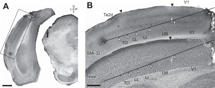
Fig. 3. — Immunohistochemistry along electrode tracks. A: section immunostained for Neurofilament protein from the animal in Fig. 1A, illustrating the position of the electrolytic lesion made at the end of our last electrode penetration. On the basis of the responses recorded during this last penetration we estimated the lesion to be 500 μm beyond the lateral border of area TO. Scale bar, 1 mm. B: detail of Neurofilament protein-labeled section from A (*top*) and adjacent Nissl-stained section (*bottom*) clearly show the location of 1 of the lesions. Functionally defined areal borders are indicated by white arrowheads along the reconstructed electrode track, while anatomically defined interareal borders between V1 and LM and LL and Te2d are indicated by black arrowheads at the cortical surface (see materials and methods for details). Scale bar, 500 μm.

Action potentials were recorded extracellularly with a Cheetah system with headstage amplifier (Neuralynx, Bozeman, MT). The signal was filtered to retain the frequencies from 300 to 4,000 Hz and digitized at 32,556 Hz. Action potentials (spikes) were recorded when they crossed a threshold set well above noise level. Recordings started from the brain surface and continued until we had penetrated through the five different areas and did not find visual responses anymore or until the animal started to show signs of stress.

During the first few penetrations in a particular rat, in order to obtain a basic idea of the retinotopy along the electrode track, we manually determined a site's population receptive field (RF) position every 200–400 μm, using continually changing shapes or small drifting circular sinusoidal gratings that could be moved across the screen. The decision to run the series of experiments at a certain site depended upon a visual inspection of the population peristimulus time histograms (PSTHs) at the site (any visible response?). Note that in principle this step of the process induces a bias to find a high proportion of responsive neurons, but typically these population histograms were dominated by low-amplitude action potentials that were not retained as single units. We recorded from sites in all five areas at different distances from the entry point.

After the recording session, spikes originating from individual units were separated off-line by KlustaKwik clustering of the spike waveforms. The input data were all the 1-ms time intervals in which the signal exceeded the trigger threshold, which was typically put at 2.35 times the standard deviation of the noise (this is an estimation based upon the average of a random sample of 25 of our recording sites). We defined single units as those clusters that were quantitatively defined by KlustaKwik and also visually obvious in the parameter space used by KlustaKwik (with parameters such as amplitude of the minimum, amplitude of the maximum, and slope). A random sample of 25 isolated clusters contained waveforms with an average peak-to-peak amplitude of 8.24 times the standard deviation of the noise (a signal-to-noise ratio of 19.07 dB; see Issa and DiCarlo 2012).

Usually, we also searched for neuronal responses to visual stimuli for ∼500 μm beyond the end of TO along our electrode track. At those locations, we were never able to find clear visual responses, by manual stimulation, systematic mapping of the RF, or showing movies of natural scenes. Sometimes we found neurons that seemed to discharge to auditory stimulation, but we did not systematically map these auditory responses.

Experiments: Visual Stimulation and Design

Stimuli were presented to the right eye on a 24-in. LCD monitor (Dell, Round Rock, TX; 1,280 × 768 pixels, frame rate = 60 Hz, mean luminance = 24 cd/m², 102° × 68°) at a distance of 20.5 cm from the eye at an angle of 40° between the rostrocaudal axis and the normal of the screen. Visual stimuli were generated and presented with custom-developed stimulation software with MATLAB (The MathWorks, Natick, MA) and the Psychophysics Toolbox (Brainard 1997; Pelli 1997). The setup was placed within a wooden cabinet to attenuate sound and light.

Experiment 1: defining optimal position.

We showed a gray shape (generally the symbol #) on a black background (Weber contrast between 1 and 13) at 15 different screen positions (3 rows by 5 columns, distributed over the screen; shape centers were spaced 26° apart). Shape diameter was 24° at the center of the screen. Each stimulus was shown for 500 ms, interspersed with a blank, black screen of equal duration plus some random jitter of up to 300 ms. The shape was randomly shown at least eight times at each position.

Experiment 2: orientation and direction tuning.

Circular drifting sinusoidal gratings of 33° diameter (Michelson contrast = 99%) were shown for 2 s on a gray background of mean luminance at the center of gravity of the RF. Twelve different drifting directions, separated by 30° and encompassing the full circle, were used. In some cases only eight drifting directions separated by 45° were used. Spatial frequency [SF; 0.04 cycles per degree (cpd)] and temporal frequency (TF; 3 Hz) were constant and chosen slightly below the mean optimal values in rat V1 (0.08 cpd and 3.8 Hz; Girman et al. 1999), since in some mouse extrastriate areas optimal SF and TF are below the values in V1 (Marshel et al. 2011). Between stimuli, a blank gray screen of mean luminance was shown for 2 s. Each drifting direction was randomly shown at least five times.

Shape experiments (experiments 3–5).

For studying shape processing, we selected six of the eight shapes from the study in monkeys by Lehky and Sereno (2007): a square, a diamond in a square, a triangle, the letter λ, the letter H, and a plus sign. The exact choice of the stimuli was based upon the neuronal responses in IT as obtained by Lehky and Sereno and included those shapes that displayed the largest variability in neural discriminability according to their data. The luminance level of each shape (i.e., the number of light pixels) was equalized by adjusting the size of each shape. The mean width of the bounding box of each shape was 27.3°, ranging from 23° to 33°. These shapes are able to drive populations of monkey anterior inferior temporal neurons, an area in monkeys that is considered the final stage of processing in the ventral stream. At the same time they are simple black and white stimuli that contain most information in the lower spatial frequencies. This allows processing by the rat visual system with its limited visual acuity.

We obtained measures of physical similarity for these shapes based on pixelwise distances (Pix) between pairs of shapes, defined as the number of pixels with a different value (binary: black or white) in the two shapes. We also determined the response of a population of simulated rat V1 neurons (V1s). For this we used a simplified version of the approach described in Pinto et al. (2008). We first smoothed the images (768 × 1,280 px) with a Gaussian low-pass filter (FWHM = 20 px, ≈1.5 cpd, the approximate acuity of our rats; see Prusky et al. 2002) and normalized to have zero mean and unit standard deviation. Next, the images were convolved with 80 filters [a combination of 5 frequencies: 0.04, 0.08, 0.15, 0.30, 0.60 cpd (Girman et al. 1999) and 16 orientations encompassing the full circle], with the size of each filter adjusted to include 2 cycles. All filters were normalized to have zero mean and norm 1. The resulting response matrix R was compared between the 15 possible pairs of shapes, and we calculated discriminability D (1 − similarity) as

D = 1 - c o r r (R_{n} (i, j, f), R_{m} (i, j, f))

where indices n and m refer to 1 of the 6 images (m > n) and index f refers to 1 of the 80 filter response planes. Indices i and j refer to image pixels in each filter response plane.

Experiment 3: estimating latency and selectivity for static shape stimuli.

The six shapes were shown in a random order for 500 ms at the optimal position within the RF (gray on black, Weber contrast between 1 and 13), interleaved with intervals of at least 500 ms of the same black background.

Experiment 4: shape selectivity for moving stimuli.

For the analysis of shape discrimination by our neuronal populations, we used the same six shapes described above, shown at identical size and contrast at the optimal position within the RF. Here, however, the shapes were shown translating along four differently oriented axes of movement, separated by 45° (horizontal, vertical, and the 2 diagonals), at constant velocity. The moving stimulus was shown for 4 s, with the movement along each axis taking 1 s at a constant speed of 48°/s. The order of the four movement axes was randomized within each 4-s presentation. During the movement along one axis, the shape started at the center (optimal) position, moved 8° (77 pixels) away from this center position in 167 ms, and then moved backward to the opposite side of the center position in 333 ms. This movement was mirrored once to complete 1 s, and then the movement seamlessly continued in a different orientation. These orientations were shuffled in each trial, resulting in 24 combinations of 6 shapes × 4 orders of orientations.

Experiment 5: position tolerance of shape selectivity.

To test the tolerance of our neuronal populations for changes in the position of the shapes within the RF, we employed an identical presentation of six shapes moving around their center position as in the previous experiment. For experiment 5, the shapes were randomly shown not only at the center RF position but also at an additional, distinct position (distance between center positions ranging from 24° to 33°). These positions were chosen so that they generated the best possible responses but had the least amount of overlap. Note that this decision was based on the online available and thus multiunit responses obtained through experiment 1. Since RF size tended to be smaller in V1 than in the extrastriate areas, the two positions were inevitably placed closer together, resulting in an overlap of the stimuli of ∼25%. Thus for V1 we might potentially measure an above-chance position tolerance due to this overlap even if V1 neurons have no position tolerance. This may occur when different edges of a particular shape have an identical orientation, such that they activate the RF similarly while the shape is at different positions.

Data Analysis

As a standard criterion, units were selected for inclusion in our data set for a particular experiment when they had a net firing rate of >2 Hz (spikes per second) for at least one of the stimuli.

Experiment 1: defining optimal position.

We determined the screen positions where the stimulus elicited a mean firing rate between 40 and 240 ms after stimulus onset that was significantly higher than baseline response, with the baseline response defined as the firing rate 200 ms prior to stimulus onset (t-test with Bonferroni correction for multiple comparisons). The optimal position was defined as the center of gravity of all the positions with a significant response, weighted for firing rate. The screen position in pixels was transformed to spherical angular coordinates of the visual field, with the right eye at the center of the sphere.

Experiment 2: orientation and direction tuning.

Net firing rate was determined by subtracting the mean baseline response from the response to each trial, with the baseline response defined as the firing rate 2 s prior to stimulus onset. For determining orientation and direction selectivity indexes (OSI and DSI), we used the net firing rate in all areas except V1, where we used either the net firing rate (F₀) or the modulation of the response (F₁) when the F₁-to-F₀ ratio was >1 for the orientation giving the strongest response for either the F₀ or F₁ component (F₁/F₀ > 1 is typically taken as the criterion to define simple cells; see Skottun et al. 1991). The OSI was calculated as follows:

OSI= \frac{R_{\max} - R_{ortho}}{R_{\max} + R_{ortho}}

where R_max is the mean net response to the preferred orientation and R_ortho is the mean net response to the orthogonal orientation (average of both directions). The DSI was defined as follows:

DSI= \frac{R_{\max} - R_{opp}}{R_{\max} + R_{opp}}

with R_max the mean net response to the preferred direction and R_opp the mean net response to the opposite direction.

Experiment 3: estimating latency and selectivity for static shape stimuli.

For estimating the cell's response latency, we first determined which shapes elicited a mean net firing rate of >2 Hz during the full 500-ms interval. Then we calculated the PSTH averaged across these shape conditions (bin width = 1 ms). After smoothing the PSTH with a Gaussian kernel (with FWHM = 3 ms), we defined the onset latency as the time point after stimulus onset where the PSTH first reached a threshold level of the baseline firing rate + 3 SD. Generally, >75 repetitions were included in our analysis.

Experiment 4: selectivity for moving shapes.

Response was calculated as the average number of spikes recorded during the 4-s stimulus presentations. Then we subtracted baseline activity, which was calculated as the average number of spikes in a 2-s interval preceding each stimulus presentation. Units were included when they showed a net response above 2 Hz for at least one of the shapes. We characterized all units by calculating several measures: mean baseline firing rate, mean raw response rate and maximal net response rates, Fano factor, max divided by mean response rate (high values indicate high selectivity), and response sparseness as described by Rolls and Tovee (1995) (low values indicate high selectivity).

a = {[\sum_{i = 1}^{n} (r_{i} / n)]}^{2} / \sum_{i = 1}^{n} (r_{i}^{2} / n)

where r_i corresponds to the baseline-subtracted and rectified response rate to the ith shape.

We also quantified the selectivity of each neuron by applying a one-way analysis of variance (ANOVA, P < 0.05) using shape as main factor and report the percentage of selective neurons out of the responsive neurons that were included in the analysis.

Experiment 5: position tolerance of shape selectivity.

We only included units whose firing rate for the most responsive shape at the least responsive position was above one-third of the response for the most responsive shape at the most responsive position. The maximally responsive shapes at both positions were not necessarily identical in order not to bias toward position tolerance. We used this one-third of the maximal response cutoff for inclusion to ensure that there was still a meaningful and significant response at the least responsive position. Performing our support vector machine (SVM) analyses without this selection criterion led to very similar results.

Calculation of sustained responses relative to peak response with static shapes (experiment 3) and moving shapes (experiment 4 or best position of experiment 5).

To compare the response to static and moving shapes, we obtained the average PSTH for each area. The PSTH of each individual cell was normalized by subtracting the average baseline response and rescaled to have a peak of height 1 before averaging, so all units contributed equally to the area average.

Neurons typically responded to a stimulus with an initial burst of spikes (onset peak), after which response continued at a lower level (sustained response). We computed the relative sustained response, which is the sustained response divided by the peak response. For this analysis we included the first 500 ms after stimulus onset for moving shapes because this was the stimulus duration of the static shapes. Per neuron, the average, baseline-subtracted PSTH (−200:500 ms) was calculated and smoothed with a Gaussian kernel with a standard deviation of 75 ms. For each cell, we located the peak time of the first transient part of the response, which we constrained between 40 and 150 ms after stimulus onset. If this interval did not contain a peak value that exceeded 3 times the standard deviation of the baseline both with static and with moving stimuli, the cell was excluded from the analysis. The percentage of neurons included was 97.6%, 87.1%, 98.5%, 87.1%, and 69.0% for areas V1, LM, LI, LL, and TO, respectively. The mean response in a 60-ms window around the peak was calculated and taken as the peak response (in Hz). We then measured the mean response in the interval between 30 ms after the peak and 500 ms after stimulus onset; we refer to this variable as the sustained response (in Hz) of the cell. The relative sustained response is calculated as the sustained response divided by the peak response. We tested for each area whether the relative sustained response was different between static and moving shapes.

Population discriminability.

Recent studies have often focused upon population discriminability to characterize neural selectivity (see, e.g., Hung et al. 2005; Li et al. 2007; Vangeneugden et al. 2011). We followed a similar approach to analyze the data from experiments 3–5. Starting with the spike count responses of a population of N neurons to P presentations of M images, each presentation of an image resulted in a response vector x with a dimensionality of N × 1, where repeated presentations (trials) of the same images can be envisioned as forming a cloud in an N-dimensional space. Linear SVMs were trained and tested in pairwise classification for each possible pair of shapes (6 shapes result in 15 unique shape pairs). A subset of the population vectors collected for both shapes were used to train the classifier. Performance was measured as the proportion of correct classification decisions for the remaining vectors not used for training (i.e., standard cross-validation; in all cases, one half of the available vectors were used for training and the other half for testing). The penalty parameter C was set to 0.5 (as in Rust and Dicarlo 2010) for every analysis; this parameter controls the trade-off between allowed training errors and margin maximalization (C = inf corresponds to a hard margin, i.e., no errors are allowed; Rychetsky 2001).

Reliability and significance of population discriminability (SVM performance).

To equalize the number of units and trials used across visual areas, we applied a resampling procedure. On every iteration, we selected a new subset of units (without replacement), with the number of units equal to the lowest number of units recorded in a single visual area with the least number of units, and a random subset of trials (without replacement). We averaged over 100 resampling iterations to obtain confidence intervals for the performance. We also computed chance performance by repeating the same analysis 1,000 times with shuffled condition labels (thus 1,000 × 100 resampling iterations).

SVM analysis of position tolerance in experiment 5.

We applied the same analysis as described above, but this time we trained an SVM classifier to discriminate two shapes at one position and measured generalization performance to the other position. To get significance estimates, we performed the same analyses after shuffling per cell the labels indicating on which position a certain trial was recorded. This will preserve the average performance correct per area, but the difference between selectivity (same position) and tolerance (over positions) will be randomized. If the actually measured difference between the two performances exceeds the 95th percentile of random differences, it is considered significant. To assess significant differences in tolerance between areas, we shuffled the area labels of the original data set for all units and repeated the same SVM analysis. When testing for differences between neighboring areas (see Table 1), we restricted the analysis to include only the data for the two areas of interest and repeated the same reshuffling procedure.

Table 1.

Summary of changes in functional properties between successive regions along the trajectory from V1 to TO

Response latency	V1	≈	LM	≈	LI	<	LL	≈	TO
Orientation selectivity	V1	≈	LM	≈	LI	<	LL	≈	TO
Direction selectivity	V1	≈	LM	<	LI	≈	LL	<	TO
Motion dependence	V1	<	LM	<	LI	≈	LL	≈	TO
Shape selectivity	V1	>	LM	≈	LI	>	LL	>	TO
Shape transformation	V1	≤	LM	≤	LI	≤	LL	≤	TO
Position tolerance	V1	≈	LM	≈	LI	≈	LL	<	TO

Open in a new tab

V1, primary visual cortex; LM, lateromedial area; LI, latero-intermediate area; LL, laterolateral area; TO, lateral occipito-temporal cortex.

Ratio between selectivity and tolerance.

We computed the ratio between the SVM performance when training and test trials come from the same position (P_selectivity) and the performance when the training and test trials come from different positions (P_tolerance). We applied a correction procedure to the two performance scores to account for the chance level obtained when guessing. We used the formula

1 - \frac{S - T}{S + T}

where S = P_selectivity − P_chance, T = P_tolerance − P_chance, and P_chance = 0.50.

To obtain confidence intervals on the difference between tolerance ratios of different areas, we shuffled the area labels of all neurons before repeating the same SVM analysis described above.

Generalization of response patterns for static stimuli to moving stimuli using SVM.

To quantify the similarity in response patterns to static and moving shapes, we trained SVM classifiers to differentiate neural responses to static shape pairs and tested performance using responses to the corresponding moving shape pair. We used the average response rate in an interval between 41 and 240 ms after stimulus onset. We also looked at the 60 ms around the onset peak, defined by looking at the average PSTH per area, to isolate the information contained in the onset transient. We limit the number of units per SVM resampling to match the number in the area with the fewest units. As before, we shuffled condition labels to obtain significance scores of individual bars.

Matching of population selectivity based on selectivity of single neurons.

To isolate the difference in tolerance between V1 and TO, we corrected for the difference in selectivity between the areas by selecting the least and most selective neurons from both areas, respectively. Selection was based on the P value obtained from an ANOVA using the net response rates at the most responsive position, where low P values indicate high selectivity. Because the amount of presentations of each shape differed over units, we applied a resampling procedure selecting 12 presentations during each iteration before calculating the P values. After averaging over 100 of these resampling iterations, the top 25 least (in V1) or most (in TO) selective units were selected for further analysis with the SVM approach detailed above.

Matching of selectivity based on ratio of responsiveness of single neurons.

To remove possible interference by the slight difference in responsiveness between positions in V1 compared with TO, we removed units with the lowest responsiveness ratio from the V1 population (n = 4). This ratio is calculated by dividing the maximum response at the least responsive position by the maximum response at the most responsive position.

Single-neuron metrics for position tolerance.

To obtain a measure of position tolerance independent of a pattern classifier as described above, we also used a traditional, single-neuron-level method to look at invariance/tolerance. An early application of this method can be found in Sary et al. (1993). To determine invariance across position, we first ordered the different stimulus conditions according to response strength for each stimulus at the preferred position. By plotting the responses with this ranking, we obtained a monotonically descending function for each neuron individually (e.g., Fig. 7) and also when we averaged responses across neurons. We normalized these responses to a scale of 0 to 1 in order to account for the previously mentioned differences in selectivity between areas. Next, we analyzed whether and how responses fall off as a function of the same ranking, but now in a different set of data obtained at a different screen position. If response preferences generalize to the other position, i.e., if there is position invariance, the function will also be descending at this second position. If there is no position invariance, the function will be more or less a flat line with no significant differences across ranks.

Fig. 7. — Responses of 2 representative neurons from V1 (A) and TO (B) to moving shapes at 2 different positions. PSTH and raster plots are shown on *left* for the shapes with the highest and lowest responses at the first position (*top*) and the same shapes at the second position (*bottom*). Horizontal black lines indicate average baseline firing rate (1 s preceding stimulus onset); horizontal red lines indicate average firing rate during the 4-s interval after stimulus onset. *Right*: net mean response rates for all shapes at the first and second stimulus positions. Both neurons show selectivity at the best position, but only in TO do we observe tolerance for position. *Insets*: mean spike waveforms.

Histology and Immunohistochemistry

At the end of the final recording session we made small electrolytic lesions (0.1 mA, 5 s, tip negative) at up to three different positions along the electrode track. One day after lesioning, the rats were given an overdose of pentobarbital sodium and transcardially perfused with 1% paraformaldehyde in PBS (0.1 M phosphate, 0.9% sodium chloride, pH 7.4), followed by 4% paraformaldehyde in PBS. Brains were removed, postfixed for 24 h in 4% paraformaldehyde, and stored in PBS.

For immunohistochemistry, all incubation and rinsing steps were performed at room temperature under gentle agitation in Tris-buffered saline (TBS; 0.01 M Tris, 0.9% NaCl, 0.3% Triton X-100, pH 7.6). Serial 50-μm-thick Vibratome sections were pretreated with 3% H₂O₂ (20 min) to neutralize endogenous peroxidase activity, rinsed, and preincubated in normal goat serum (1:5, 45 min; Chemicon International). The sections were then incubated overnight with the monoclonal antibody SMI-32 (1:8,000; Covance Research Products, Berkeley, CA; Sternberger and Sternberger 1983). Detection was performed with biotinylated goat anti-mouse IgGs (1:200, 30 min; Dako, Glostrup, Denmark) and a streptavidin-horseradish peroxidase solution (1:500, 1 h; Dako). The sections were immunostained with the glucose oxidase-diaminobenzidine-nickel method, resulting in a gray-black staining (Shu et al. 1988; Van der Gucht et al. 2007). After the sections were mounted on gelatin-coated slides, they were left to dry. The sections were then dehydrated with graded ethanol, after which they were cleared in xylene and coverslipped with DePeX.

For histology, serial sections adjacent to the immunostained sections were mounted on gelatin-coated slides, dehydrated in graded ethanol, and rinsed in distilled water. The sections were briefly Nissl stained in a filtered 1% cresyl violet solution (1%; Fluka Chemical, Sigma-Aldrich) to determine the layers of the rat neocortex and the position of the electrolytic lesions. For differentiation between gray and white matter, they were then rinsed in distilled water with a few drops of acetic acid. Finally, the sections were dehydrated, cleared with xylene, and coverslipped with DePeX. Photographs of the histological and immunostained patterns were obtained with a Zeiss Axio-Imager equipped with a Zeiss Axiocam.

The border between V1 and lateral extrastriate cortex was anatomically defined based on both Nissl and SMI-32 staining patterns (Sia and Bourne 2008; Van der Gucht et al. 2007), while the anatomical demarcation of Te2d and extrastriate visual cortex was based on the comparison of the SMI-32 immunological staining pattern with that obtained by Sia and Bourne (2008). Recording sites and borders between V1, LM, LI, LL, and TO were then reconstructed based on the position of the electrolytic lesions and the recording depths along the electrode track.

The anatomical characterization of the fifth physiologically differentiated area (TO) was as follows. The posterior subdivision of TeA is often referred to as Te2 (Zilles 1990) and was recently further subdivided into a dorsal and a ventral part based upon SMI-32 staining (Sia and Bourne 2008), with the dorsal part being visually responsive. Since we found correspondence between the LL/TO border in our SMI-32 staining and the V2L/Te2d border obtained with the same marker by Sia and Bourne (2008), our fifth visually responsive area is probably part of the visually active dorsal subdivision Te2d of Sia and Bourne (2008). However, since the size of TO was quite small (<500 μm along the electrode track in the coronal plane), it seems unlikely that Te2d and this fifth area completely coincide. We therefore have tentatively named this region TO (temporal occipital area) referring to its location at the border of temporal and occipital cortex.

Control of Retinal Stimulation

In our experiments, we mostly avoided eye movement confounds by the characteristics of our animal model, the visual stimulation parameters, and the presence of appropriate control comparisons. The assumptions behind this methodology were checked later in a separate control experiment in which we explicitly measured eye position.

In light of previous studies (Niell and Stryker 2010; Zoccolan et al. 2010), we expected that eye position could be ignored, as is done in many studies, both anesthetized and awake (Andermann et al. 2011; Marshel et al. 2011; Niell and Stryker 2008), because rodents only make occasional eye movements. Most importantly, these eye movements are not related to stimulus onset and other stimulus characteristics as long as the stimuli are small enough, as in our study, to avoid reflexive kinetic responses.

In our study, the recordings in V1 already provide a useful baseline for comparisons with all other areas. If eye movements were abundant, which would not be in line with the previous studies referred to above, then it might, e.g., be difficult to find small RFs. Similarly, it would be difficult to find simple cells with phase-dependent responses, as the preferred phase would depend upon eye position at an ever finer scale. Nevertheless, we recorded small RFs in V1. Furthermore, the ratio of simple to complex cells in our study was similar to this ratio in previously published studies of rodent V1 despite the fact that we did not optimize our gratings for SF, TF, or size (Fig. 4, A and B; 44 simple vs. 116 complex cells, 27.5%; Girman et al. 1999; Niell and Stryker 2008; Van den Bergh et al. 2010; Van Hooser et al. 2005). In sum, any effects of eye movements in our study are very likely small. Finally, all our conclusions are based upon comparisons between V1 and other areas. We expect potential effects of eye movements to be present during the V1 recordings as much as during the recordings in other areas.

Fig. 4. — Simple and complex cells in rat V1 and eye movements. A: example peristimulus time histogram (PSTH) of a simple cell in V1 [modulation of the response (F₁)/net firing rate (F₀) = 1.16], responding to a drifting grating of optimal orientation. Black and white bars indicate that the stimulus is off or on, respectively. B: frequency distribution of F₁/F₀ of V1 neurons (n = 160). C: example eye movement trace, showing the distance in degrees between the pupil center and the median pupil position. Stimulus onset and offset (*experiment 5*, shapes at 2 different positions, indicated as blue and red bars) are plotted below the trace, showing that there is no correlation between eye movements and stimulus position. Eye movements were very small compared with the distance between the 2 stimulus positions (*right y*-axis). About 79% of this trace falls within 1.25° from the central position, which is slightly above the overall average of 75% (see *inset*).

As a direct test, we measured eye movements in the separate control experiments in which we recorded from different cortical depths in V1 (orthogonal penetrations). Eye movements were recorded with a CCD camera (Prosilica GC660) fitted with a motorized zoom lens (Navitar Zoom 6000) and an infrared filter (Thorlabs FEL0800). Pupil positions were extracted with an online MATLAB algorithm running at 30 Hz. Both the setup and the pupil extraction routines were based on Zoccolan et al. (2010).

The eye tracking confirmed our expectations that eye movements were not so frequent, stimulus independent, and relatively small. In particular, the characteristics of eye movements in typical traces turned out to be very similar to previously published findings (Chelazzi et al. 1989; Niell and Stryker 2010; Zoccolan et al. 2010). For most of the time (75%), eye position was at one particular central position (within 1.25° from the median X and Y position for the whole trace). For the remainder of the time, small eye movements occurred away from the central position and mostly in a horizontal direction, sometimes followed by a slower gradual drift back to the central position. An example trace is shown in Fig. 4C, illustrating how small these eye movements are compared with the stimulus size and the distance between the screen positions in the test for position tolerance.

Given these findings, we expect that the occurrence of eye movements would not substantially affect the outcome of our analyses. We tested this directly using neural responses acquired together with eye position recordings (no. of neurons per functional property: RF size = 26; OSI/DSI = 35; position tolerance = 22). We compared the outcome for analyses that included all trials versus analyses that only included trials without any change in eye position from the most common central position. Also including the trials with a change in eye position did not change RF size [no. of positions with significant response: 2.58 in the trials without eye movement compared with 2.85 in all trials, t(25) = 1.2721; P = 0.2150], nor did it change any of the other indexes obtained with grating stimuli (OSI: 0.443 ± 0.035 vs. 0.435 ± 0.037; DSI: 0.380 ± 0.049 vs. 0.382 ± 0.044). Position invariance was also not affected by the presence of small eye movements: After ranking stimuli according to response strength at a first screen position, the difference between the best and worst stimulus at a second position (computed in the same way as for the main data, where this difference was 1.59 ± 0.72 Hz) was very small both for trials without eye movements (difference of 1.04 ± 0.66 Hz) and for all trials (difference of 1.59 ± 0.72 Hz), and a direct statistical comparison revealed no significant effect of including the trials with eye movements [t(21) = −1.2669; P = 0.2191].

Of course, by not finding an effect we cannot exclude the possibility that there is a small effect of eye movements (even though we used a sensitive measurement by searching for the effect of eye movements in the same neurons with a paired t-test). In fact, a very small effect should be there in, e.g., RF size when measured with a much more dense grid of screen positions, and the results above show a small nonsignificant effect in the expected direction for both RF size and position invariance. Thus we do not conclude that there are no effects of eye movement in our data, but we conclude that such effects, if they are present, are very small and do not have effects with a size that would meaningfully affect our results and conclusions.

RESULTS

Here we first establish a progression of five visual areas, starting with V1 and including extrastriate areas LM, LI, LL, and TO. Response properties that are typically studied in area V1, such as latency and orientation and direction selectivity already provide clear evidence for a progressive change in response properties across these five areas. By moving toward response properties typically studied in higher-level visual regions in primates, such as shape selectivity and position tolerance, we demonstrate commonalities with higher-level processing in primates. In addition, however, our data also show that this shape selectivity is restricted to moving shapes and is accompanied by a strong selectivity for direction of motion.

A Progression of Four Physiologically Distinct Visual Areas Lateral to V1

We performed extracellular single-unit recordings in V1 and several more lateral visual areas in awake rats. We sampled neuronal populations from different extrastriate visual areas (LM, LI, and LL; Espinoza and Thomas 1983) that are located progressively farther from V1 (Fig. 1), in contrast to most other areas identified in mice that form a ring bordering V1. Since in mouse the homologous areas LM and LI are part of the ventral stream (Wang et al. 2012), we hypothesized that these areas together with more lateral areas might be involved in visual object processing.

As described previously (Espinoza and Thomas 1983; Thomas and Espinoza 1987), these different areas are easily identified in single electrode tracks based on retinotopy. Two detailed example tracks are shown in Fig. 2, A and B, starting dorsomedially and then moving ventrolaterally during a recording session. We defined the retinotopic position of each recording site by a manual mapping. Typically, a quantitative estimation of optimal location at the recorded sites was performed through experiment 1 (# symbol presented at 15 positions, see materials and methods). Using both methods, we observed an ordered progression of the RFs along our electrode tracks in all animals. Every area was marked by a distinguishable pattern of RF locations: moving from periphery to center along the azimuthal axis in odd areas (V1, LI) or vice versa in even areas (LM and LL) (Fig. 2, A–C), accompanied by shifts in vertical RF position at some areal borders {median elevation in LM and LL was respectively higher and lower than in V1 and LI [Kruskal-Wallis (KW), P < 0.0001]; mean elevation V1 = 25.4 ± 0.8, LM = 33.6 ± 1.0, LI = 21.8 ± 0.9, LL = 8.0 ± 0.9}. For V1 and the first three lateral areas LM, LI, and LL, this pattern of RF locations corresponds with the literature (Espinoza and Thomas 1983; Montero 1993; Olavarria and Montero 1984; Thomas and Espinoza 1987; Vaudano et al. 1991). In addition, we found a small visually responsive area along our electrode track beyond LL, which we could not relate to any area characterized in earlier studies. We tentatively called it TO (temporal occipital area) because it was located at the border of visual occipital cortex and the temporal association area Te2d (Fig. 3). Although the mean response rate here was lower, we again observed a mirroring of this area's retinotopy compared with that in LL (Fig. 2). RF elevation in TO was also higher than in LL (mean elevation TO = 23.3 ± 1.2). The retinotopy was very clear along single tracks and was consistent over time with different penetrations (for examples, see Fig. 2).

Through experiment 1 we also obtained a rough estimate of RF size in each of the visual areas (Fig. 5A). We limited our analysis to V1, LI, and TO, since the location of RFs at the top or bottom edge of the screen in LM and LL would result in an underestimation of the RF size. Although experiment 1 was not perfectly suited for a determination of RF size given the relatively coarse (only 15 positions) and restricted (only the part of the visual field enclosed by the monitor) sampling of the visual field, RF size expressed by the number of screen positions with significant response was larger in areas LI (3.22 ± 0.12 positions, mean data ± SE) and TO (3.64 +± 0.27 positions) than in V1 (2.00 ± 0.09 positions) (KW, P < 0.0001; Fig. 5B). Comparing cell populations with firing rates matched across these areas confirmed these results (RF size in V1: 2.00 ± 0.10 positions; LI: 3.18 ± 0.13 positions; TO: 3.65 ± 0.27 positions). We did not find a relation between RF size and eccentricity, but this null result has to be interpreted with caution as screen size limited the recorded RF size at the peripheral edge of the screen. Interestingly, while all V1 neurons had small RFs, the range of RF sizes in TO seemed to be much larger. Not only did we observe a number of small RFs, a substantial number of TO cells had very large RFs as well, resulting in a very widespread distribution of RF sizes in TO—a phenomenon that has also been observed in monkey inferior temporal cortex (Op De Beeck and Vogels 2000).

We determined onset latency in all five areas with static shapes (experiment 3: 6 geometric shapes presented at the most responsive position out of 15 mapped in experiment 1; see Fig. 5, C and D). Mean onset latency was 45.1 ± 1.3 ms in V1 (mean data ± SE) (Fig. 5D). No significant higher onset latencies were found in LM and LI. LL and TO showed substantially higher response latencies than V1, LM, and LI (KW, P < 0.0001; mean latency in LM = 48.4 ± 1.7 ms, LI = 49.5 ± 1.0 ms, LL = 67.4 ± 2.5 ms, and TO = 73.9 ± 3.6 ms; see Fig. 5D). We confirmed these findings for cell populations with matched firing rates across all areas (mean latency: V1 = 47.1 ± 2.0 ms, LM = 49.8 ± 1.9 ms, LI = 51.2 ± 1.3 ms, LL = 67.9 ± 2.8 ms, and TO = 74.6 ± 3.8 ms).

Finally, we tested the orientation and direction tuning of neurons in all five areas, using drifting gratings with SF and TF that were kept constant across areas (experiment 2). The tuning is summarized by OSI and DSI (see Fig. 5, E–H). The data show that orientation selectivity in V1 was 0.40 ± 0.02, it tended to be higher in LM (0.49 ± 0.03; Wilcoxon signed-rank test, P = 0.0136, Bonferroni-corrected criterion for significance = 0.005), and it showed a marked and significant (P = 0.0001) increase in LI (0.55 ± 0.02). More laterally, LL (0.65 ± 0.03) and TO (0.69 ± 0.03) had an even higher OSI than the other three areas (KW, P < 0.0001). After matching for similar net firing rates, comparable results were obtained (e.g., OSI increasing from 0.44 ± 0.02 in V1 to 0.69 ± 0.03 in TO). Even more strikingly, DSI was rather low in V1 (0.29 ± 0.02) but progressively increased along our electrode tracks, resulting in strongly direction-selective units in TO (0.76 ± 0.03). Moreover, DSI was significantly different between almost all visual areas, except for LI (0.54 ± 0.02) and LL (0.63 ± 0.03) and V1 and LM (0.40 ± 0.03) (KW, P < 0.0001). Again, similar differences were found if we analyzed cell populations of the distinct areas matched for net response rate (e.g., DSI increasing from 0.34 ± 0.02 in V1 to 0.77 ± 0.03 in TO).

We report analyses controlling for maximal net response rate, since maximal net response rate showed the strongest differences between V1, LM, and LI versus the more lateral areas LL and TO (Fig. 5K; median maximal net response rate in the orientation tuning experiment). There were much less significant differences between areas for spontaneous firing rate (Fig. 5I), maximal raw firing rate (Fig. 5J), or Fano factor (Fig. 5L).

Note that with the penetrations used for all our experiments detailed here in results, we end up with differences among areas in the laminar distribution of the recorded neurons. Figure 1B shows a tentative distribution of our recordings, revealing that such differences are minor between the four extrastriate areas, with mostly recordings in the lower layers. In contrast, V1 stands out by being sampled mostly in the upper layers. We performed an additional control study in V1 in which we implemented all our experiments and compared the findings between the upper and lower layers. None of the area differences mentioned up to this point was found to be explainable by the presence of laminar differences in area V1. More specifically, onset latency was not different between upper and lower layers [KW, P = 0.7189; mean onset latency upper layers: 29.30 ± 0.91 ms (n = 47), lower layers: 30.49 ± 1.21 ms (n = 53); both latencies are lower compared with V1 latency reported in experiment 3 because stimulus luminance was higher for this control experiment], and neither were OSI and DSI [OSI (KW, P = 0.6050): mean OSI upper layers 0.40 ± 0.03 (n = 58), lower layers 0.43 ± 0.03 (n = 62); DSI (KW, P = 0.8480): mean DSI upper layers 0.33 ± 0.03 (n = 58), lower layers 0.35 ± 0.03 (n = 62)].

Static vs. Moving Shapes

All the analyses above help to functionally characterize the five areas and suggest that they are processing information hierarchically. Next, we investigated the shape processing capabilities of these areas. In primates experiments are typically performed with static shapes; however, when starting with that approach we noticed that in particular the higher areas showed little sustained response to static shapes. We decided to have each of six shapes move around a central point during 4 s. This manipulation hardly affected the average strength of the sustained responses in V1 (see Fig. 6, A, C, and E), but for higher areas we found an increase of the sustained response compared with the static condition (see Fig. 6, B, D, and F).

Fig. 6. — Static shapes elicit little sustained response in higher areas. *A–D*: single-unit responses to static and moving shapes. For static shapes, we show the raster plots for the whole 500-ms stimulus presentation; for moving shapes, we show the comparable window of the first 500 ms of the full 4,000-ms presentation duration. Vertical green line indicates stimulus onset. Horizontal black lines indicate average baseline firing rate (200 ms preceding stimulus onset); horizontal red lines indicate average firing rate during the 500-ms interval after stimulus onset. The number of trials varied for static shapes between 25 and 26 and for moving shapes between 12 and 13. Example neurons are the same as shown in Fig. 7. The example V1 neuron shows strong responses to static (A) and moving (C) shapes. The example TO neuron (B and D) shows little sustained response to static shapes, except for an initial transient, and a more sustained and selective response to moving shapes. E and F: comparison of average traces in response to static or moving stimuli in V1 (E) and highest area, TO (F). G: normalized sustained response to static and moving shapes in the different areas, averaged across all neurons (error bars indicate SE). H: SVM classifier performances when using data for moving and static shapes; equal intervals (500 ms) were used to calculate response rates. Red bars indicate threshold for significance of individual bars. Asterisks indicate significant differences between bars, calculated by shuffling experiment labels.

To test this explicitly, we compared the responses to static shapes (experiment 3: 6 shapes presented during 500 ms) with the responses to moving shapes (experiment 4: same 6 shapes presented translating over a central position during 4 s), using the neurons that were tested in both experiments. We averaged peak-normalized traces of all units in each area, and we measured the level of sustained response relative to the peak for both “static shape” and “moving shape” conditions for the first 500 ms after stimulus onset (Fig. 6G). We performed an ANOVA with “area” as a between-neuron factor with five levels (V1, LM, LI, LL, TO), “static versus moving” as a within-neuron factor, and the relative sustained response as the dependent variable. There was a highly significant main effect of static versus moving [F(1,362) = 376.08, P < 0.0001]. This difference was present in each area individually (post hoc testing, each P < 0.0001). There was a small main effect of area [F(4,362) = 2.58, P < 0.05], which was strongly modulated by a highly significant interaction between area and static versus moving [F(4,362) = 13.783, P < 0.0001]. In sum, the relative sustained response was higher for moving compared with static stimuli, an effect that was most pronounced in the areas beyond V1. These sustained responses to moving shapes also allow for better decoding of shape information compared with the responses to static shapes in all areas except V1 (Fig. 6H).

Shape Selectivity: Single-Unit Responses

To test for shape selectivity, we presented six moving shapes at one or two responsive positions (experiments 4 and 5, respectively) while we recorded from 631 (114, 104, 166, 107, and 140 for areas V1, LM, LI, LL, and TO, respectively) neurons. After selecting responsive neurons to which each shape had been presented at least 12 times, we retained 413 single units (88, 63, 131, 68, and 63). The percentage of responsive neurons was 77%, 61%, 79%, 64%, and 45% for areas V1, LM, LI, LL, and TO, respectively. In the case where experiment 5 was conducted, we selected the data from the most responsive position. The responses of two example units from V1 and TO to these shapes are shown in Fig. 7 (see position 1 data). These illustrate that a sizable percentage of the units in each of the areas demonstrated significant selectivity (62.9%, 56.5%, 76.1%, 51.4%, and 38.7%, respectively). Although the mean spontaneous response rates show some variation over areas in this experiment, no significant differences were found (Fig. 8A). Maximal raw response rates were significantly different between LI and TO; all other comparisons proved nonsignificant (Fig. 8B). The clearest difference in maximal net response rates was that units in V1 and LI had on average higher maximum net response rates than those in areas LM, LL, and TO (Fig. 8C). When we examined the Fano factors per area, this was greater in area TO compared with all other areas (see Fig. 8D). These results were similar to what we found for the orientation tuning experiment (see above and Fig. 5, K and L).

Fig. 8. — Population data of single-unit indicators of shape selectivity. *A–D*: median values of spontaneous activity (A), maximal raw firing rate (B), maximal net firing rate (C), and Fano factor (D) in all areas obtained during the presentation of moving shapes (see Fig. 7). E: median ratio of net response rates for the shape with maximal response rate over the mean net response rate of all shapes. F: frequency distribution of maximum-to-mean response ratio. G: median response sparseness for the 6 different shapes. H: frequency distribution of response sparseness. Error bars in *A–E* and G indicate confidence intervals. *Statistical significance (Wilcoxon signed-rank test P < 0.05, Bonferroni corrected for multiple comparisons). F and H, *left*: closed triangles represent the mean and open diamonds the medians of the population response property. *Right*: statistical significance of pairwise comparisons of median response property (Wilcoxon signed-rank test) for each visual area (*P < 0.05, Bonferroni corrected for multiple comparisons).

We quantify selectivity of single cells with two different measures: maximal response divided by mean response (max-to-mean ratio) and response sparseness (Rolls and Tovee 1995; see materials and methods). Both measures indicate that the selectivity of single units goes up from V1 to area TO (Fig. 8, E–G; note the reversed interpretation for response sparseness). Since selectivity for oriented gratings also increased from V1 to TO, we compared max/mean for the shapes and the drifting gratings, obtained from the same cells (Fig. 9). In most areas max/mean, i.e., the selectivity for the different stimuli, was higher for the drifting gratings than for the shapes. However, this could be due to a different sampling of the stimulus space for grating orientations and objects. The range of the stimulus space that we sampled for oriented gratings was defined and complete (the full circle of orientations), whereas for the (rather similar) objects we probably only sampled a small subset of this space.

Fig. 9. — Relation between selectivity for oriented drifting gratings and shapes: comparison between max-to-mean response ratios for drifting gratings vs. moving shapes for the 5 visual areas. Histograms indicate the difference in the max-to-mean response ratios between moving shapes and drifting gratings. In most areas max/mean, i.e., the selectivity for the different stimuli, was higher for the drifting gratings than for the shapes.

Shape Selectivity: Population-Level Analysis

In recent years, the belief has grown that neural information tends to be distributed over many neurons and that analysis of neural data should be designed to account for this coding scheme. We further quantified shape selectivity by multivariate, population-level analyses (Hung et al. 2005; Rust and Dicarlo 2010; Vangeneugden et al. 2011). We obtained a measure of population discriminability for each of the 15 shape pairs from linear classification methods (SVMs with 63 units per SVM resampling; see materials and methods). Low SVM performance (around chance level = 0.50) is indicative of highly similar population responses to the shapes, whereas a high SVM performance (maximal performance = 1.00) indicates that it is easy to discriminate between the shapes based on the population responses. Average (across all 15 pairs) SVM performance scores per area were 0.93, 0.87, 0.88, 0.82, and 0.70 for areas V1, LM, LI, LL, and TO, respectively (see Fig. 10A). When we analyzed the data from the orthogonal recordings in V1, we obtained results comparable with those for V1 from the oblique penetrations [upper layers (V1U): 0.94; lower layers (V1L): 0.92; Fig. 10A]. Red lines in Fig. 10A indicate 95% significance thresholds based on 1,000 permutations using shuffled condition labels (V1-TO: 0.512, 0.511, 0.509, 0.511, 0.513 and V1U-V1L: 0.512, 0.511). Thus, similarly to what we found with the single-unit measure of selectivity, neuronal populations from all areas were selective to differences between the shapes. These data also indicate that the ability to detect differences between shapes, here referred to as selectivity, goes down in higher areas. This is not in agreement with the single-unit measures constructed with the same data. This apparent contradiction may be partially resolved by considering that the average Fano factor increases toward TO. Single-unit measures are obtained by averaging over all responses, effectively ignoring trial-to-trial variability. Our SVM analysis is sensitive to this variability, which may give different results. Including trial-to-trial variability may give a more realistic view of the information that is available to the organism at a given point in time. Alternatively, the possibility exists that we could have observed better SVM classification performances in TO versus V1 when using more complex or naturalistic shapes. We report the results of both analyses, as both complement each other and give a more comprehensive view of neural processing.

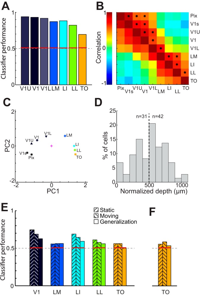
Fig. 10. — Gradual change in information readout over different areas. A: SVM classifier pairwise discrimination performance (averaged across 15 shape pairs) per area, including upper and lower layers of V1 (V1U and V1L). Red lines indicate significance levels obtained through permutations. Dashed line indicates chance level. B: correlation matrix based on dissimilarity scores for 15 shape pairs based on physical stimulus properties (Pix and V1s) and neural responses (in areas V1, LM, LI, LL, and TO and V1U and V1L). C: plot of the first 2 principal components computed for the correlation matrix shown in B. This representation indicates that upper layers of V1 are more similar to physical measures; lower layers code the shapes more like area LM, downstream to V1. D: depth distribution of neurons in orthogonal V1 penetrations for units used in V1U and V1L. Depth is normalized for small differences in electrode tilt. Dashed line indicates division between upper (V1U; *left*) and lower (V1L; *right*) layers. E: SVM classifier discrimination performance averaged over 15 shape pairs per area using the initial peak response (41–240 ms after stimulus onset) only. *Left* bars show discrimination performance for static stimuli, *center* bars show discrimination performance for moving stimuli, and *right* bars show the classifier generalization from static to moving stimuli, obtained after training the SVM classifier on responses to static shapes and testing this classifier on responses to the moving shape. Red lines indicate significance levels obtained through permutations. Dashed line indicates chance level. There is significant generalization from static to moving stimuli in all areas except for TO. In F we show the same generalization data for TO, but here only the responses in a 60-ms interval around the population PSTH peak were used. Significant generalization was observed.

Shape Selectivity: Comparison Between Areas

Population responses for different shapes, the vector of response strengths across all neurons, are not identical, which is how different shapes can be discriminated. Some pairs of shapes are more discriminable than other shape pairs. We analyzed how the pattern of neuronal discriminability across shape pairs changes over areas. Within an hierarchical organization, each transition to a next area typically corresponds to a transformation of the information. This successive transformation enables the visual cortex to extract certain features that may carry behavioral relevance (e.g., presence of an object) at the expense of other properties (e.g., location in the visual field).

We correlated the pattern of variation in neural discriminability across the 15 shape pairs in a given area with first-order measures of (dis)similarity (Pix and V1s; see materials and methods) between these same shape pairs, as these measures capture what can be extracted from the retinal stimulation with purely linear or first-order processing, and with neural discriminability in other areas. The resulting correlation matrix gives an indication of which stimulus properties were represented in each area and visualizes how the representation of stimuli changed across the five cortical areas. All correlations are shown in Fig. 10B.

First, we compared the variation in neural discriminability in each of the five areas with first-order measures of similarity (Pix and V1s). Across the 15 shape pairs, V1 correlated with Pix (r = 0.49, P = 0.03) and V1s (r = 0.61, P = 0.01), while other areas showed little to no correlation to Pix (LM: r = −0.01, P = 0.47; LI: r = −0.18, P = 0.27; LL: r = −0.14, P = 0.34; TO: r = −0.32, P = 0.13) or to V1s (LM: r = −0.12, P = 0.35; LI: r = −0.25, P = 0.19; LL: r = −0.30, P = 0.17; TO: r = −0.41, P = 0.06). Probabilities are based on statistics using permuted data (see materials and methods).

Second, we compared the variation in neural discriminability among the five areas. Pairwise correlations among areas suggested that neighboring areas (e.g., V1 and LM) tended to correlate (V1-LM: r = 0.21, P = 0.24; LM-LI: r = 0.65, P = 0.01; LI-LL: r = 0.48, P = 0.05; LL-TO: r = 0.52, P = 0.05) better than areas that are further apart (average r = 0.24).

These analyses revealed that area V1 processes shapes in terms of simple local properties as they are captured by pixel-based similarity (Pix) and the simulated V1 filters (V1s) and that this representation is gradually transformed along the progression of five areas. To further visualize this overall pattern, we subjected the similarity matrix shown in Fig. 10B to principal component analysis (PCA). The resulting spatial representation, shown in Fig. 10C, illustrates the close correspondence between V1 and Pix/V1s and the gradual progression from V1 to TO.

We performed a similar analysis with the V1 data from the orthogonal penetrations in which we distinguished between upper and lower layers (Fig. 10D). Using these new (nonoverlapping) V1 data we find a further finer transition within V1 itself so that the representation in the upper layers is most similar to pix/V1s while lower layers are already shifted partially toward the extrastriate regions (see Fig. 10, A–D).

In this experiment we showed moving instead of stationary shapes, since moving shapes elicited more sustained responses that led to better decoding of the information in the responses. Evidently, this results in uncertainty as to whether it is the shape information or the movement of the shapes that drives the discrimination performance of the SVM classifier in the different areas. To understand the effect of the shape itself on the discrimination performance, we performed a generalization test from static to moving stimuli based on the 41–240 ms interval after stimulus onset (the peak response for both static and moving stimuli; see Fig. 6, E and F). With this interval, the SVM discrimination performance was roughly equal for both the static and moving stimulus conditions (Fig. 10E, left and middle bars, respectively). We then trained the SVM classifier on responses in this interval to the static stimuli and tested the performance of the discrimination classifier on the responses to the moving stimuli (N cells: V1: 59, LM: 63, LI: 97, LL: 56, TO: 39; 39 per SVM resampling). Although most areas showed a small drop in performance compared with the standard test where training and test conditions are the same, almost all areas, except for TO, showed a generalization performance that is above the significance levels defined by permutations on the data (for details see materials and methods). This finding indicates that in V1, LM, LI, and LL shape information from the static stimuli is at least partially responsible for the SVM performance when we presented the shapes in a moving fashion. In TO the most discriminable feature of moving shapes at this response interval seems to be related to motion, as a classifier trained on stationary shapes fails to generalize to moving shapes. Nevertheless, when we performed the same generalization analysis in TO but with responses in a shorter interval of 60 ms around the peak of the population PSTH for this individual area (Fig. 6F), we did find significant generalization as well (Fig. 10F). Thus in TO at least some of the SVM performance for moving shapes at the early response interval can be explained by response to the shape itself.

Shape Selectivity and Position Invariance

We performed experiment 5 in which we presented the six shapes at two positions, the optimal position and a second, distinct position that was still within the RF but was sufficiently far away from the first position to reduce overlap of the shapes shown at both locations (Fig. 7). We selected neurons that showed sufficient responses at both positions (see materials and methods), which yielded 258 units (38, 25, 96, 49, and 50 per area; with 25 units per SVM resampling). The percentage of selective neurons was 63.2%, 56.0%, 77.9%, 52.0%, and 44.0% for areas V1, LM, LI, LL, and TO, respectively. Figure 7 illustrates the responses of two selective V1 and TO neurons.

These data allowed the comparison of the response to stimuli at the same position (selectivity), similar to the analysis in the previous section. In addition, we now also used the responses at one position to train a classifier and test classification performance at the other position (tolerance). If the five areas along our recording track form a hierarchy as in the primate ventral visual pathway stream (Felleman and Van Essen 1991) (e.g., H-Max; Riesenhuber and Poggio 1999), then we expect no or very limited position tolerance in V1 when stimuli are presented at different nonoverlapping positions and more position tolerance in area TO. Figure 7A shows that in V1 shape selectivity is modulated by position, while this selectivity is maintained for the TO example neuron (Fig. 7B), indicative of position tolerance.

As shown in Fig. 11A, the discrimination performance within the same position was comparable to what was found for the larger population (results shown in Fig. 10A); however, performances were lower because of the decreased number of neurons used to train and test the classifier (25 instead of 63). As before, SVM performance using data from a single position decreased somewhat along the five areas. However, while discrimination performance decreased, tolerance performance did not (Fig. 11A, shaded bars). We summarized position tolerance for each area by the ratio of SVM performance across positions versus within a single position, corrected for guessing (see materials and methods, Fig. 11B). This ratio indicates how much information is retained after moving to another position and would be “0” when no information is retained and “1” in the case of perfect position invariance. The ratio increased along the hierarchy of five areas, with a ratio close to “1” in area TO.

Using this ratio index, we normalize the differences in discriminability between the visual areas. This index is subject to the criticism that the main effect is the decrease in discrimination performance from V1 to TO, not an increase in tolerance performance. To address this problem we implemented another method in which the SVM analysis is restricted to subsets of neurons with matched selectivity. We restricted the SVM analysis to a subset of neurons with either good or poor single-neuron selectivity. In area V1 we selected the 25 neurons with the poorest selectivity, and in area TO we selected the neurons with the best selectivity. The resulting subpopulation shape discriminability of these two visual areas were similar (V1: 72%, TO: 68%; P = 0.24). Nevertheless, when we used this subpopulation to test for position tolerance we again observed a much larger performance decrease in V1 when the classifiers had to generalize across positions (P < 0.01, based on 100 permutations; see Fig. 11C). In this new analysis, the absolute tolerance performance differed among areas, with a significantly (P < 0.01) higher generalization to the untrained position (tolerance) in TO (72%) compared with V1 (56%).

Note that we selected two RF positions in V1 with above-baseline responsiveness. Given that RF size tended to be smaller in V1, we put the two positions closer together for V1 than for other areas (average distance: V1 20.7 ± 0.5°, LM 18.2 ± 0.7°, LI 25.8 ± 0.9°, LL 28.4 ± 1.3°, TO 23.5 ± 0.8°; % of overlap between stimuli: V1 25.9 ± 1.4, LM 19.9 ± 1.5, LI 12.1 ± 1.7, LL 9.5 ± 1.3, TO 8.4 ± 1.1). For LM, since only part of the RF was present on the screen, we could stimulate only the part of the RF that was generally located along the top edge of the screen. As a consequence of this methodology, the ratio of responsiveness between the two RF positions that we included was relatively similar in area V1 and in area TO (V1: 0.74 ± 0.03; TO: 0.79 ± 0.02). If we removed the small remaining difference in this ratio of responsiveness by matching the V1 and TO neurons, the difference in position tolerance (ratio between within-position and across-position tests) remained significant (P < 0.01). Thus the increase in position tolerance from V1 to TO is not caused by an increased RF size but comes on top of any increase in RF size.

Finally, the increase in tolerance relative to selectivity is accompanied by an increase in correlation between selectivity and tolerance for individual pairs (correlation in V1 = 0.52, LM = −0.01, LI = 0.58, LL = 0.69, TO = 0.97; see Fig. 11D). This finding suggests that population responses to stimuli at different positions in the RF get more and more similar as we move up the hierarchy.

To corroborate the findings from the population-level analyses described above, we also used single-unit metrics (Fig. 11E). First, for each unit, we sorted the different stimulus conditions with respect to the strength of the response to that stimulus for one position. The solid line in Fig. 11E represents the mean over all units of the responses as a function of rank for the position that was used to determine the ranking, normalized between 1 and 0. Then we applied the same ranking and response normalization to the data from the second position (dashed line in Fig. 11E). The question is whether there is a significantly stronger response to the higher-ranked stimuli at this second position for all units in each brain area. Already in area V1, we find a stronger response to rank 1 than to rank 6. To assess the significance of this difference, we compared the observed difference between rank 1 and rank 6 with the distribution of differences based upon permuting the stimulus labels of these two ranks (based upon 10,000 permutations). The observed difference was unlikely to occur by chance (P = 0.038). Thus, as in the population-level analyses, the single-neuron metric shows some position tolerance in area V1. According to the same permutation test on the difference in responsiveness between rank 1 and rank 6, all other brain areas also showed a significantly stronger response at rank 1 compared with rank 6 (LM: P = 0.011; LI: P < 0.0001; LL: P < 0.0001; TO: P < 0.0001). Finally, we explicitly compared the difference in response between rank 1 and rank 6 between areas V1 and TO, using a permutation test in which we shuffled the area to which each neuron was assigned (as was also done for the population-level analyses). This analysis revealed a stronger position tolerance in TO compared with V1 (P = 0.026). In sum, the single-neuron-level analyses corroborate the findings from the population-level analyses: 1) significant position tolerance in all brain areas V1, LM, LI, LL, and TO and 2) a stronger position tolerance in TO compared with V1.

DISCUSSION

We described a progression of five visual areas in rat cortex that might contain a functional hierarchy in terms of how shape is processed. Some of these changes happen gradually across the five areas; other changes occur more stepwise, in which case the steps do not always occur at the same level. In Table 1 we summarize the most important changes along the trajectory from V1 to TO. Overall, we confirmed several key properties that have previously been identified in the ventral “object vision” pathway in primates and some properties that are clearly very different between primates and rodents. First, there is an increase in the position tolerance of shape selectivity that goes beyond the tolerance that can be expected given simple RF properties. Second, there is a gradual transition from the V1 representation of the shapes in terms of local physical stimulus properties, similar to the responses of a bank of local spatial filters (De Valois and De Valois 1988) and to pixel-based measures of shape differences, to a representation that shows gradually less similarity to the V1 representation. Third, we did not find evidence for a segregation of form and motion processing in the rodent, with even an increased dependence upon the presence of motion and its direction in area TO compared with area V1. Finally, even up to area TO we find strong selectivity for simple stimuli such as sinusoidal gratings, suggesting that even the most lateral visually responsive regions in the rat temporal cortex do not show a similar preference for complex stimuli as found in the ventral visual pathway in primates.

Identity and Nomenclature of Five Visual Areas from V1 to TO

Our recordings span five visual areas: V1, LM, LI, LL, and TO. The first three areas, V1, LM, and LI, have been identified in many studies, including studies in mice (Wang et al. 2009, 2012; Wang and Burkhalter 2007). These three areas are easily found with tracer injections in V1. Wang and Burkhalter (2007) also showed an increase in RF size from V1 to LI. Recent imaging work in mice has revealed marked functional differences between these areas (Andermann et al. 2011; Marshel et al. 2011). Area LL was first investigated in older electrophysiological work in rats (Espinoza and Thomas 1983; Montero 1993; Thomas and Espinoza 1987; Vaudano et al. 1991). We also identified a fifth physiologically differentiated area, TO.

The anatomical position and the functional properties of these five areas suggest that they form a functional hierarchy. However, to establish a true hierarchy the functional data will have to be corroborated with anatomical connectivity. Interestingly, a recent study (Wang et al. 2012) suggested an anatomical hierarchy from V1 over LM to LI, which then fed into the more posterior areas P and POR (postrhinal cortex); LL and TO have not been identified in mice. These connectivity data in mice, when extrapolated to rats, suggest two potential situations. First, LL and TO could receive direct input from area LI and as such form a five-area pathway from V1 (over LI) to TO that would run in parallel with a pathway from V1 (over LI) to POR. Second, LL and TO could receive input from area POR and no direct input from area LI. In that case, we would have a seven-area pathway of which we have only recorded five areas. This second option would be consistent with our observation that there is a large increase in response latency between LI and LL/TO.

Finally, we have very limited information about the area we refer to as TO. First and foremost, we only have functional data showing a particular retinotopic organization that suggests the presence of a specific area and no anatomical or connectivity information. These data, however, could be used as a starting point for a tracer injection study that could provide this connectivity information. Second, within each single animal, we only have a very limited view of the retinotopic map. As in the other areas, our electrode penetration results in a clear retinotopic progression of the horizontal position of RFs in TO. The mapping of vertical position is not possible with our methods. However, a parsimonious solution would be to extrapolate the scheme of Espinoza and Thomas (1983) for LI and LL to TO, so that in TO there would be a full map of a hemifield with vertical position mapped from posterior to anterior coordinates.

Areal Differences in Selectivity for Gratings

We found a gradual increase in both orientation and direction selectivity from V1 to TO. Compared with previous studies in mice, the mean DSI in V1 was very similar. For orientation selectivity in V1, we found a lower level than Niell and Stryker (2008) or Van den Bergh et al. (2010) but a level very similar to that observed by Marshel et al. (2011). There are several differences between studies, and in particular all these mouse studies were done in anesthetized animals. In terms of choice of stimuli our approach is most similar to that of Marshel et al. (2011), because they also used fixed SF and TF for determining orientation tuning for all cells. The other studies determined orientation selectivity by using gratings with the cell's optimal SF (but a fixed TF). Our fixed SF, which is lower than the optimal SF in rat V1 (Girman et al. 1999), might make the orientations of the grating less defined in V1, resulting in lower OSI measurements. Moreover, using a SF lower than the cell's optimal in V1 might potentially drive the cells to respond to an untuned detection signal, leading to lower OSI in V1 than in the more lateral areas that potentially prefer lower SF. We did not directly investigate tuning for SF in rats, but in mice there is no significant difference in optimal SF between V1 and LI (Marshel et al. 2011). Consequently, any differences in OSI levels, at least between V1 and LI, will probably not be the result of differences in SF. Direction tuning, on the other hand, does not seem to be influenced by the SF used, as DSI measures in V1 in all studies were similar, independent of optimizing the gratings for SF. As a result, the DSI measurements in LM to TO will not be influenced by possible differences in preferred SF in these areas, either.

Finally, and maybe most importantly in the present context, even if part of the increase in orientation and direction selectivity toward TO were explainable by the exact choice of grating parameters, it is striking that this selectivity for gratings is going up instead of going down as is typically observed in the primate visual system when investigating areas with an increasing distance from V1. This could suggest that even in the most lateral temporal visual cortex of rodents complex stimuli are not as strongly preferred as in the primate ventral visual pathway. Of course, we cannot exclude the possibility that in rodents complex stimuli are only strongly represented in these areas when they become behaviorally relevant. Since our animals were only passively viewing the stimuli (i.e., they were not running in place and generally did not make body movements unless a water reward was given), further studies that use complex shapes in a behaviorally relevant task that might also require locomotion while recording from these lateral visual areas will be required to elucidate this question.

It might also be useful to know how much of the shape selectivity could be explained by the orientation selectivity. We did not explicitly test this because the small set of objects we used with a limited number of biased orientations (mostly cardinal and a few diagonal lines) would make this analysis not very convincing with the present data. A specifically designed experiment would be required to address this in detail. This would fall outside the scope of the present study. However, to some extent we did analyze whether a bias in lines in the objects would explain the shape selectivity. The simulated V1 responses (V1s) are highly dependent on the oriented lines within the stimuli. When these responses correlate well with the population SVM performance (as in V1), we can assume that orientation bias in the objects might affect the object selectivity. However, outside of V1, there is no correlation with V1s, suggesting that orientation bias does not play much of a role.

Tolerance to Image Transformations

There is an increase of position tolerance from V1 to TO. In area TO, the position tolerance was much higher than in area V1. This position tolerance provides a neural analog of the position tolerance that has been observed behaviorally in recent studies using rats (Tafazoli et al. 2012; Vermaercke and Op de Beeck 2012).

In primates and humans there is a large literature on position tolerance (for review, see Kravitz et al. 2008). In addition, studies have investigated the tolerance to many other image transformations, such as tolerance for changes in size (Ito et al. 1995), illumination (Braje et al. 1998), in-plane orientation (Guyonneau et al. 2006; Knowlton et al. 2009), and orientation in depth (Logothetis et al. 1994; Wallis and Bulthoff 2001; Wang et al. 2005). In light of behavioral work from Zoccolan and colleagues (Alemi-Neissi et al. 2013; Zoccolan et al. 2009), we also expect some tolerance to these other transformations somewhere in the rat visual cortex, and on the basis of our present data we hypothesize to find this tolerance to be the strongest in and around area TO. Nevertheless, because of the possibly more specialized object recognition abilities of primates compared with rodents, the degree of tolerance in the rat visual system might be lower than the tolerance found very high up in the monkey ventral visual pathway.

No Segregation of Form and Motion in Rat Visual Cortex?

In several respects we find very obvious differences with primates. First, tests with moving gratings show a gradual increase in orientation and motion selectivity toward area TO. In contrast, the orientation selectivity for gratings is very low in monkey IT cortex (Vogels and Orban 1994). Second, neurons in rat visual cortex, and in particular in extrastriate regions, are hardly selective to stationary shapes. In addition, the sustained responses to moving stimuli are also influenced by the motion trajectory of the shapes (see, e.g., the responses of the example TO neuron shown in Fig. 7). In contrast, neurons in monkey IT cortex show clear selectivity and partially sustained responses to stationary shapes. While the segregation of form and motion signals is not absolute even in the primate system (see, e.g., the modulation of the responses in the ventral region by stimulus motion, Schultz and Pilz 2009), it is clearly much more clear-cut than what we see in rat visual cortex, at least as far as this particular succession of five visual areas is concerned and for the stimuli employed in this study.

An investigation of the exact characteristics of motion processing is beyond the scope of the present study. For example, by limiting our stimuli to only one speed of motion, visual areas with different preferred speeds of motion might show lower responses to our stimuli than when using stimuli moving at the optimal speed. There is not much known about the details of preferred speed of motion in rat visual cortex. Still, even with speed of motion and other motion parameters as important factors to be investigated further, it is already clear that motion is a very important stimulus feature for all of the five investigated areas. However, rodent visual cortex might partially inherit the strong and distributed motion selectivity from properties of precortical visual processing, such as the abundance of receptors with transient responses. Nevertheless, part of the motion selectivity is created in cortex, as responses and selectivity were more strongly affected by motion in area TO than in area V1. Further studies will be needed to better understand how motion is represented in these regions and how the motion sensitivity interacts with other factors such as the behavioral relevance of the stimuli.

Conclusions

We identified a progression of five visual areas in rat cortex along which there is an increase of position tolerance and a gradual transformation of the selectivity to moving shapes. This selectivity was most strongly observed for moving shapes. In combination, these findings reveal striking commonalities and differences with object processing in the primate ventral visual pathway and in computational models of object recognition (e.g., Riesenhuber and Poggio 1999). While many questions remain unresolved, our findings provide a first step toward a full characterization of the functional specialization in the lateral regions of the visual cortex in rodents.

GRANTS

This work was funded by the Human Frontier Science Program (Grant CDA-0040/2008), the Research Council Leuven (Grants CREA/07/004 and GOA/12/008), and the Fund for Scientific Research FWO-Flanders (Grant G.0562.10). B. Vermaercke was supported by a postdoctoral fellowship from the Research Council Leuven and is currently a postdoctoral fellow of FWO-Flanders.

DISCLOSURES

No conflicts of interest, financial or otherwise, are declared by the author(s).

AUTHOR CONTRIBUTIONS

Author contributions: B.V., F.J.G., H.P.O.d.B., and G.V.d.B. conception and design of research; B.V., F.J.G., E.Y., and G.V.d.B. performed experiments; B.V. and G.V.d.B. analyzed data; B.V., E.Y., L.A., H.P.O.d.B., and G.V.d.B. interpreted results of experiments; B.V. and G.V.d.B. prepared figures; B.V., H.P.O.d.B., and G.V.d.B. drafted manuscript; B.V., H.P.O.d.B., and G.V.d.B. edited and revised manuscript; B.V., F.J.G., E.Y., L.A., H.P.O.d.B., and G.V.d.B. approved final version of manuscript.

ACKNOWLEDGMENTS

The authors thank D. Balschun, R. D'Hooge, and the members of the Laboratory of Biological Psychology for their support during the implementation of this research and R. Vogels for his comments on an earlier version of this text.

REFERENCES

Alemi-Neissi A, Rosselli FB, Zoccolan D. Multifeatural shape processing in rats engaged in invariant visual object recognition. J Neurosci 33: 5939–5956, 2013 [DOI] [PMC free article] [PubMed] [Google Scholar]
Andermann ML, Kerlin AM, Roumis DK, Glickfeld LL, Reid RC. Functional specialization of mouse higher visual cortical areas. Neuron 72: 1025–1039, 2011 [DOI] [PMC free article] [PubMed] [Google Scholar]
Brainard DH. The Psychophysics Toolbox. Spat Vis 10: 433–436, 1997 [PubMed] [Google Scholar]
Braje WL, Kersten D, Tarr MJ, Troje NF. Illumination effects in face recognition. Psychobiology 26 371–380, 1998 [Google Scholar]
Chelazzi L, Rossi F, Tempia F, Ghirardi M, Strata P. Saccadic eye movements and gaze holding in the head-restrained pigmented rat. Eur J Neurosci 1: 639–646, 1989 [DOI] [PubMed] [Google Scholar]
De Valois RL, De Valois KK. Spatial Vision. Oxford, UK: Oxford Univ. Press, 1988 [Google Scholar]
Dicarlo JJ, Zoccolan D, Rust NC. How does the brain solve visual object recognition? Neuron 73: 415–434, 2012 [DOI] [PMC free article] [PubMed] [Google Scholar]
Espinoza SG, Thomas HC. Retinotopic organization of striate and extrastriate visual cortex in the hooded rat. Brain Res 272: 137–144, 1983 [DOI] [PubMed] [Google Scholar]
Felleman DJ, Van Essen DC. Distributed hierarchical processing in the primate cerebral cortex. Cereb Cortex 1: 1–47, 1991 [DOI] [PubMed] [Google Scholar]
Girman SV, Sauve Y, Lund RD. Receptive field properties of single neurons in rat primary visual cortex. J Neurophysiol 82: 301–311, 1999 [DOI] [PubMed] [Google Scholar]
Goodale MA, Milner AD. Separate visual pathways for perception and action. Trends Neurosci 15: 20–25, 1992 [DOI] [PubMed] [Google Scholar]
Guyonneau R, Kirchner H, Thorpe SJ. Animals roll around the clock: the rotation invariance of ultrarapid visual processing. J Vis 6: 1008–1017, 2006 [DOI] [PubMed] [Google Scholar]
Hung CP, Kreiman G, Poggio T, DiCarlo JJ. Fast readout of object identity from macaque inferior temporal cortex. Science 310: 863–866, 2005 [DOI] [PubMed] [Google Scholar]
Issa EB, DiCarlo JJ. Precedence of the eye region in neural processing of faces. J Neurosci 32: 16666–16682, 2012 [DOI] [PMC free article] [PubMed] [Google Scholar]
Ito M, Tamura H, Fujita I, Tanaka K. Size and position invariance of neuronal responses in monkey inferotemporal cortex. J Neurophysiol 73: 218–226, 1995 [DOI] [PubMed] [Google Scholar]
Knowlton BJ, McAuliffe SP, Coelho CJ, Hummel JE. Visual priming of inverted and rotated objects. J Exp Psychol Learn Mem Cogn 35: 837–848, 2009 [DOI] [PubMed] [Google Scholar]
Kravitz DJ, Vinson LD, Baker CI. How position dependent is visual object recognition? Trends Cogn Sci 12: 114–122, 2008 [DOI] [PubMed] [Google Scholar]
Lehky SR, Sereno AB. Comparison of shape encoding in primate dorsal and ventral visual pathways. J Neurophysiol 97: 307–319, 2007 [DOI] [PubMed] [Google Scholar]
Li S, Ostwald D, Giese M, Kourtzi Z. Flexible coding for categorical decisions in the human brain. J Neurosci 27: 12321–12330, 2007 [DOI] [PMC free article] [PubMed] [Google Scholar]
Logothetis NK, Pauls J, Bulthoff HH, Poggio T. View-dependent object recognition by monkeys. Curr Biol 4: 401–414, 1994 [DOI] [PubMed] [Google Scholar]
Marshel JH, Garrett ME, Nauhaus I, Callaway EM. Functional specialization of seven mouse visual cortical areas. Neuron 72: 1040–1054, 2011 [DOI] [PMC free article] [PubMed] [Google Scholar]
Mishkin M, Ungerleider LG. Contribution of striate inputs to the visuospatial functions of parieto-preoccipital cortex in monkeys. Behav Brain Res 6: 57–77, 1982 [DOI] [PubMed] [Google Scholar]
Montero VM. Retinotopy of cortical connections between the striate cortex and extrastriate visual areas in the rat. Exp Brain Res 94: 1–15, 1993 [DOI] [PubMed] [Google Scholar]
Niell CM, Stryker MP. Highly selective receptive fields in mouse visual cortex. J Neurosci 28: 7520–7536, 2008 [DOI] [PMC free article] [PubMed] [Google Scholar]
Niell CM, Stryker MP. Modulation of visual responses by behavioral state in mouse visual cortex. Neuron 65: 472–479, 2010 [DOI] [PMC free article] [PubMed] [Google Scholar]
Olavarria J, Montero VM. Relation of callosal and striate-extrastriate cortical connections in the rat: morphological definition of extrastriate visual areas. Exp Brain Res 54: 240–252, 1984 [DOI] [PubMed] [Google Scholar]
Op De Beeck HP, Vogels R. Spatial sensitivity of macaque inferior temporal neurons. J Comp Neurol 426: 505–518, 2000 [DOI] [PubMed] [Google Scholar]
Pelli DG. The VideoToolbox software for visual psychophysics: transforming numbers into movies. Spat Vis 10: 437–442, 1997 [PubMed] [Google Scholar]
Pinto N, Cox DD, DiCarlo JJ. Why is real-world visual object recognition hard? PLoS Comput Biol 4: e27, 2008 [DOI] [PMC free article] [PubMed] [Google Scholar]
Prusky GT, Harker KT, Douglas RM, Whishaw IQ. Variation in visual acuity within pigmented, and between pigmented and albino rat strains. Behav Brain Res 136: 339–348, 2002 [DOI] [PubMed] [Google Scholar]
Riesenhuber M, Poggio T. Hierarchical models of object recognition in cortex. Nat Neurosci 2: 1019–1025, 1999 [DOI] [PubMed] [Google Scholar]
Rolls ET, Tovee MJ. Sparseness of the neuronal representation of stimuli in the primate temporal visual cortex. J Neurophysiol 73: 713–726, 1995 [DOI] [PubMed] [Google Scholar]
Rust NC, Dicarlo JJ. Selectivity and tolerance (“invariance”) both increase as visual information propagates from cortical area V4 to IT. J Neurosci 30: 12978–12995, 2010 [DOI] [PMC free article] [PubMed] [Google Scholar]
Rychetsky M. Algorithms and Architectures for Machine Learning Based on Regularized Neural Networks and Support Vector Approaches. Berlin: Shaker, 2001, p. 259 [Google Scholar]
Sary G, Vogels R, Orban GA. Cue-invariant shape selectivity of macaque inferior temporal neurons. Science 260: 995–997, 1993 [DOI] [PubMed] [Google Scholar]
Schultz J, Pilz KS. Natural facial motion enhances cortical responses to faces. Exp Brain Res 194: 465–475, 2009 [DOI] [PMC free article] [PubMed] [Google Scholar]
Shu SY, Ju G, Fan LZ. The glucose oxidase-DAB-nickel method in peroxidase histochemistry of the nervous system. Neurosci Lett 85: 169–171, 1988 [DOI] [PubMed] [Google Scholar]
Sia Y, Bourne JA. The rat temporal association cortical area 2 (Te2) comprises two subdivisions that are visually responsive and develop independently. Neuroscience 156: 118–128, 2008 [DOI] [PubMed] [Google Scholar]
Skottun BC, De Valois RL, Grosof DH, Movshon JA, Albrecht DG, Bonds AB. Classifying simple and complex cells on the basis of response modulation. Vision Res 31: 1079–1086, 1991 [DOI] [PubMed] [Google Scholar]
Sternberger LA, Sternberger NH. Monoclonal antibodies distinguish phosphorylated and nonphosphorylated forms of neurofilaments in situ. Proc Natl Acad Sci USA 80: 6126–6130, 1983 [DOI] [PMC free article] [PubMed] [Google Scholar]
Tafazoli S, Di Filippo A, Zoccolan D. Transformation-tolerant object recognition in rats revealed by visual priming. J Neurosci 32: 21–34, 2012 [DOI] [PMC free article] [PubMed] [Google Scholar]
Thomas HC, Espinoza SG. Relationships between interhemispheric cortical connections and visual areas in hooded rats. Brain Res 417: 214–224, 1987 [DOI] [PubMed] [Google Scholar]
Van den Bergh G, Zhang B, Arckens L, Chino YM. Receptive-field properties of V1 and V2 neurons in mice and macaque monkeys. J Comp Neurol 518: 2051–2070, 2010 [DOI] [PMC free article] [PubMed] [Google Scholar]
Van der Gucht E, Hof PR, Van Brussel L, Burnat K, Arckens L. Neurofilament protein and neuronal activity markers define regional architectonic parcellation in the mouse visual cortex. Cereb Cortex 17: 2805–2819, 2007 [DOI] [PubMed] [Google Scholar]
Van Hooser SD, Heimel JA, Nelson SB. Functional cell classes and functional architecture in the early visual system of a highly visual rodent. Prog Brain Res 149: 127–145, 2005 [DOI] [PubMed] [Google Scholar]
Vangeneugden J, De Maziere PA, Van Hulle MM, Jaeggli T, Van Gool L, Vogels R. Distinct mechanisms for coding of visual actions in macaque temporal cortex. J Neurosci 31: 385–401, 2011 [DOI] [PMC free article] [PubMed] [Google Scholar]
Vaudano E, Legg CR, Glickstein M. Afferent and efferent connections of temporal association cortex in the rat: a horseradish peroxidase study. Eur J Neurosci 3: 317–330, 1991 [DOI] [PubMed] [Google Scholar]
Vermaercke B, Op de Beeck HP. A multivariate approach reveals the behavioral templates underlying visual discrimination in rats. Curr Biol 22: 50–55, 2012 [DOI] [PubMed] [Google Scholar]
Vogels R, Orban GA. Activity of inferior temporal neurons during orientation discrimination with successively presented gratings. J Neurophysiol 71: 1428–1451, 1994 [DOI] [PubMed] [Google Scholar]
Wallis G, Bulthoff HH. Effects of temporal association on recognition memory. Proc Natl Acad Sci USA 98: 4800–4804, 2001 [DOI] [PMC free article] [PubMed] [Google Scholar]
Wang G, Obama S, Yamashita W, Sugihara T, Tanaka K. Prior experience of rotation is not required for recognizing objects seen from different angles. Nat Neurosci 8: 1768–1775, 2005 [DOI] [PubMed] [Google Scholar]
Wang L, Rangarajan KV, Lawhn-Heath CA, Sarnaik R, Wang BS, Liu X, Cang J. Direction-specific disruption of subcortical visual behavior and receptive fields in mice lacking the beta2 subunit of nicotinic acetylcholine receptor. J Neurosci 29: 12909–12918, 2009 [DOI] [PMC free article] [PubMed] [Google Scholar]
Wang Q, Burkhalter A. Area map of mouse visual cortex. J Comp Neurol 502: 339–357, 2007 [DOI] [PubMed] [Google Scholar]
Wang Q, Sporns O, Burkhalter A. Network analysis of corticocortical connections reveals ventral and dorsal processing streams in mouse visual cortex. J Neurosci 32: 4386–4399, 2012 [DOI] [PMC free article] [PubMed] [Google Scholar]
Zilles K. Anatomy of the neocortex: cytoarchitecture and myeloarchitecture. In: The Cerebral Cortex of the Rat, edited by Kolb B, Tees RC. Cambridge, MA: MIT Press, 1990, p. 77–112 [Google Scholar]
Zoccolan D, Graham BJ, Cox DD. A self-calibrating, camera-based eye tracker for the recording of rodent eye movements. Front Neurosci 4: 193, 2010 [DOI] [PMC free article] [PubMed] [Google Scholar]
Zoccolan D, Oertelt N, DiCarlo JJ, Cox DD. A rodent model for the study of invariant visual object recognition. Proc Natl Acad Sci USA 106: 8748–8753, 2009 [DOI] [PMC free article] [PubMed] [Google Scholar]

[B1] Alemi-Neissi A, Rosselli FB, Zoccolan D. Multifeatural shape processing in rats engaged in invariant visual object recognition. J Neurosci 33: 5939–5956, 2013 [DOI] [PMC free article] [PubMed] [Google Scholar]

[B2] Andermann ML, Kerlin AM, Roumis DK, Glickfeld LL, Reid RC. Functional specialization of mouse higher visual cortical areas. Neuron 72: 1025–1039, 2011 [DOI] [PMC free article] [PubMed] [Google Scholar]

[B3] Brainard DH. The Psychophysics Toolbox. Spat Vis 10: 433–436, 1997 [PubMed] [Google Scholar]

[B4] Braje WL, Kersten D, Tarr MJ, Troje NF. Illumination effects in face recognition. Psychobiology 26 371–380, 1998 [Google Scholar]

[B5] Chelazzi L, Rossi F, Tempia F, Ghirardi M, Strata P. Saccadic eye movements and gaze holding in the head-restrained pigmented rat. Eur J Neurosci 1: 639–646, 1989 [DOI] [PubMed] [Google Scholar]

[B6] De Valois RL, De Valois KK. Spatial Vision. Oxford, UK: Oxford Univ. Press, 1988 [Google Scholar]

[B7] Dicarlo JJ, Zoccolan D, Rust NC. How does the brain solve visual object recognition? Neuron 73: 415–434, 2012 [DOI] [PMC free article] [PubMed] [Google Scholar]

[B8] Espinoza SG, Thomas HC. Retinotopic organization of striate and extrastriate visual cortex in the hooded rat. Brain Res 272: 137–144, 1983 [DOI] [PubMed] [Google Scholar]

[B9] Felleman DJ, Van Essen DC. Distributed hierarchical processing in the primate cerebral cortex. Cereb Cortex 1: 1–47, 1991 [DOI] [PubMed] [Google Scholar]

[B10] Girman SV, Sauve Y, Lund RD. Receptive field properties of single neurons in rat primary visual cortex. J Neurophysiol 82: 301–311, 1999 [DOI] [PubMed] [Google Scholar]

[B11] Goodale MA, Milner AD. Separate visual pathways for perception and action. Trends Neurosci 15: 20–25, 1992 [DOI] [PubMed] [Google Scholar]

[B12] Guyonneau R, Kirchner H, Thorpe SJ. Animals roll around the clock: the rotation invariance of ultrarapid visual processing. J Vis 6: 1008–1017, 2006 [DOI] [PubMed] [Google Scholar]

[B13] Hung CP, Kreiman G, Poggio T, DiCarlo JJ. Fast readout of object identity from macaque inferior temporal cortex. Science 310: 863–866, 2005 [DOI] [PubMed] [Google Scholar]

[B14] Issa EB, DiCarlo JJ. Precedence of the eye region in neural processing of faces. J Neurosci 32: 16666–16682, 2012 [DOI] [PMC free article] [PubMed] [Google Scholar]

[B15] Ito M, Tamura H, Fujita I, Tanaka K. Size and position invariance of neuronal responses in monkey inferotemporal cortex. J Neurophysiol 73: 218–226, 1995 [DOI] [PubMed] [Google Scholar]

[B16] Knowlton BJ, McAuliffe SP, Coelho CJ, Hummel JE. Visual priming of inverted and rotated objects. J Exp Psychol Learn Mem Cogn 35: 837–848, 2009 [DOI] [PubMed] [Google Scholar]

[B17] Kravitz DJ, Vinson LD, Baker CI. How position dependent is visual object recognition? Trends Cogn Sci 12: 114–122, 2008 [DOI] [PubMed] [Google Scholar]

[B18] Lehky SR, Sereno AB. Comparison of shape encoding in primate dorsal and ventral visual pathways. J Neurophysiol 97: 307–319, 2007 [DOI] [PubMed] [Google Scholar]

[B19] Li S, Ostwald D, Giese M, Kourtzi Z. Flexible coding for categorical decisions in the human brain. J Neurosci 27: 12321–12330, 2007 [DOI] [PMC free article] [PubMed] [Google Scholar]

[B20] Logothetis NK, Pauls J, Bulthoff HH, Poggio T. View-dependent object recognition by monkeys. Curr Biol 4: 401–414, 1994 [DOI] [PubMed] [Google Scholar]

[B21] Marshel JH, Garrett ME, Nauhaus I, Callaway EM. Functional specialization of seven mouse visual cortical areas. Neuron 72: 1040–1054, 2011 [DOI] [PMC free article] [PubMed] [Google Scholar]

[B22] Mishkin M, Ungerleider LG. Contribution of striate inputs to the visuospatial functions of parieto-preoccipital cortex in monkeys. Behav Brain Res 6: 57–77, 1982 [DOI] [PubMed] [Google Scholar]

[B23] Montero VM. Retinotopy of cortical connections between the striate cortex and extrastriate visual areas in the rat. Exp Brain Res 94: 1–15, 1993 [DOI] [PubMed] [Google Scholar]

[B24] Niell CM, Stryker MP. Highly selective receptive fields in mouse visual cortex. J Neurosci 28: 7520–7536, 2008 [DOI] [PMC free article] [PubMed] [Google Scholar]

[B25] Niell CM, Stryker MP. Modulation of visual responses by behavioral state in mouse visual cortex. Neuron 65: 472–479, 2010 [DOI] [PMC free article] [PubMed] [Google Scholar]

[B26] Olavarria J, Montero VM. Relation of callosal and striate-extrastriate cortical connections in the rat: morphological definition of extrastriate visual areas. Exp Brain Res 54: 240–252, 1984 [DOI] [PubMed] [Google Scholar]

[B27] Op De Beeck HP, Vogels R. Spatial sensitivity of macaque inferior temporal neurons. J Comp Neurol 426: 505–518, 2000 [DOI] [PubMed] [Google Scholar]

[B28] Pelli DG. The VideoToolbox software for visual psychophysics: transforming numbers into movies. Spat Vis 10: 437–442, 1997 [PubMed] [Google Scholar]

[B29] Pinto N, Cox DD, DiCarlo JJ. Why is real-world visual object recognition hard? PLoS Comput Biol 4: e27, 2008 [DOI] [PMC free article] [PubMed] [Google Scholar]

[B30] Prusky GT, Harker KT, Douglas RM, Whishaw IQ. Variation in visual acuity within pigmented, and between pigmented and albino rat strains. Behav Brain Res 136: 339–348, 2002 [DOI] [PubMed] [Google Scholar]

[B31] Riesenhuber M, Poggio T. Hierarchical models of object recognition in cortex. Nat Neurosci 2: 1019–1025, 1999 [DOI] [PubMed] [Google Scholar]

[B32] Rolls ET, Tovee MJ. Sparseness of the neuronal representation of stimuli in the primate temporal visual cortex. J Neurophysiol 73: 713–726, 1995 [DOI] [PubMed] [Google Scholar]

[B33] Rust NC, Dicarlo JJ. Selectivity and tolerance (“invariance”) both increase as visual information propagates from cortical area V4 to IT. J Neurosci 30: 12978–12995, 2010 [DOI] [PMC free article] [PubMed] [Google Scholar]

[B34] Rychetsky M. Algorithms and Architectures for Machine Learning Based on Regularized Neural Networks and Support Vector Approaches. Berlin: Shaker, 2001, p. 259 [Google Scholar]

[B35] Sary G, Vogels R, Orban GA. Cue-invariant shape selectivity of macaque inferior temporal neurons. Science 260: 995–997, 1993 [DOI] [PubMed] [Google Scholar]

[B36] Schultz J, Pilz KS. Natural facial motion enhances cortical responses to faces. Exp Brain Res 194: 465–475, 2009 [DOI] [PMC free article] [PubMed] [Google Scholar]

[B37] Shu SY, Ju G, Fan LZ. The glucose oxidase-DAB-nickel method in peroxidase histochemistry of the nervous system. Neurosci Lett 85: 169–171, 1988 [DOI] [PubMed] [Google Scholar]

[B38] Sia Y, Bourne JA. The rat temporal association cortical area 2 (Te2) comprises two subdivisions that are visually responsive and develop independently. Neuroscience 156: 118–128, 2008 [DOI] [PubMed] [Google Scholar]

[B39] Skottun BC, De Valois RL, Grosof DH, Movshon JA, Albrecht DG, Bonds AB. Classifying simple and complex cells on the basis of response modulation. Vision Res 31: 1079–1086, 1991 [DOI] [PubMed] [Google Scholar]

[B40] Sternberger LA, Sternberger NH. Monoclonal antibodies distinguish phosphorylated and nonphosphorylated forms of neurofilaments in situ. Proc Natl Acad Sci USA 80: 6126–6130, 1983 [DOI] [PMC free article] [PubMed] [Google Scholar]

[B41] Tafazoli S, Di Filippo A, Zoccolan D. Transformation-tolerant object recognition in rats revealed by visual priming. J Neurosci 32: 21–34, 2012 [DOI] [PMC free article] [PubMed] [Google Scholar]

[B42] Thomas HC, Espinoza SG. Relationships between interhemispheric cortical connections and visual areas in hooded rats. Brain Res 417: 214–224, 1987 [DOI] [PubMed] [Google Scholar]

[B43] Van den Bergh G, Zhang B, Arckens L, Chino YM. Receptive-field properties of V1 and V2 neurons in mice and macaque monkeys. J Comp Neurol 518: 2051–2070, 2010 [DOI] [PMC free article] [PubMed] [Google Scholar]

[B44] Van der Gucht E, Hof PR, Van Brussel L, Burnat K, Arckens L. Neurofilament protein and neuronal activity markers define regional architectonic parcellation in the mouse visual cortex. Cereb Cortex 17: 2805–2819, 2007 [DOI] [PubMed] [Google Scholar]

[B45] Van Hooser SD, Heimel JA, Nelson SB. Functional cell classes and functional architecture in the early visual system of a highly visual rodent. Prog Brain Res 149: 127–145, 2005 [DOI] [PubMed] [Google Scholar]

[B46] Vangeneugden J, De Maziere PA, Van Hulle MM, Jaeggli T, Van Gool L, Vogels R. Distinct mechanisms for coding of visual actions in macaque temporal cortex. J Neurosci 31: 385–401, 2011 [DOI] [PMC free article] [PubMed] [Google Scholar]

[B47] Vaudano E, Legg CR, Glickstein M. Afferent and efferent connections of temporal association cortex in the rat: a horseradish peroxidase study. Eur J Neurosci 3: 317–330, 1991 [DOI] [PubMed] [Google Scholar]

[B48] Vermaercke B, Op de Beeck HP. A multivariate approach reveals the behavioral templates underlying visual discrimination in rats. Curr Biol 22: 50–55, 2012 [DOI] [PubMed] [Google Scholar]

[B49] Vogels R, Orban GA. Activity of inferior temporal neurons during orientation discrimination with successively presented gratings. J Neurophysiol 71: 1428–1451, 1994 [DOI] [PubMed] [Google Scholar]

[B50] Wallis G, Bulthoff HH. Effects of temporal association on recognition memory. Proc Natl Acad Sci USA 98: 4800–4804, 2001 [DOI] [PMC free article] [PubMed] [Google Scholar]

[B51] Wang G, Obama S, Yamashita W, Sugihara T, Tanaka K. Prior experience of rotation is not required for recognizing objects seen from different angles. Nat Neurosci 8: 1768–1775, 2005 [DOI] [PubMed] [Google Scholar]

[B52] Wang L, Rangarajan KV, Lawhn-Heath CA, Sarnaik R, Wang BS, Liu X, Cang J. Direction-specific disruption of subcortical visual behavior and receptive fields in mice lacking the beta2 subunit of nicotinic acetylcholine receptor. J Neurosci 29: 12909–12918, 2009 [DOI] [PMC free article] [PubMed] [Google Scholar]

[B53] Wang Q, Burkhalter A. Area map of mouse visual cortex. J Comp Neurol 502: 339–357, 2007 [DOI] [PubMed] [Google Scholar]

[B54] Wang Q, Sporns O, Burkhalter A. Network analysis of corticocortical connections reveals ventral and dorsal processing streams in mouse visual cortex. J Neurosci 32: 4386–4399, 2012 [DOI] [PMC free article] [PubMed] [Google Scholar]

[B55] Zilles K. Anatomy of the neocortex: cytoarchitecture and myeloarchitecture. In: The Cerebral Cortex of the Rat, edited by Kolb B, Tees RC. Cambridge, MA: MIT Press, 1990, p. 77–112 [Google Scholar]

[B56] Zoccolan D, Graham BJ, Cox DD. A self-calibrating, camera-based eye tracker for the recording of rodent eye movements. Front Neurosci 4: 193, 2010 [DOI] [PMC free article] [PubMed] [Google Scholar]

[B57] Zoccolan D, Oertelt N, DiCarlo JJ, Cox DD. A rodent model for the study of invariant visual object recognition. Proc Natl Acad Sci USA 106: 8748–8753, 2009 [DOI] [PMC free article] [PubMed] [Google Scholar]

PERMALINK

Functional specialization in rat occipital and temporal visual cortex

Ben Vermaercke

Florian J Gerich

Ellen Ytebrouck

Lutgarde Arckens

Hans P Op de Beeck

Gert Van den Bergh

Abstract

MATERIALS AND METHODS

Animal Preparation, Surgery, and Habituation

Fig. 1.

Electrophysiological Recordings

Fig. 2.

Fig. 3.

Experiments: Visual Stimulation and Design

Experiment 1: defining optimal position.

Experiment 2: orientation and direction tuning.

Shape experiments (experiments 3–5).

Experiment 3: estimating latency and selectivity for static shape stimuli.

Experiment 4: shape selectivity for moving stimuli.

Experiment 5: position tolerance of shape selectivity.

Data Analysis

Experiment 1: defining optimal position.

Experiment 2: orientation and direction tuning.

Experiment 3: estimating latency and selectivity for static shape stimuli.

Experiment 4: selectivity for moving shapes.

Experiment 5: position tolerance of shape selectivity.

Calculation of sustained responses relative to peak response with static shapes (experiment 3) and moving shapes (experiment 4 or best position of experiment 5).

Population discriminability.

Reliability and significance of population discriminability (SVM performance).

SVM analysis of position tolerance in experiment 5.

Table 1.

Ratio between selectivity and tolerance.

Generalization of response patterns for static stimuli to moving stimuli using SVM.

Matching of population selectivity based on selectivity of single neurons.

Matching of selectivity based on ratio of responsiveness of single neurons.

Single-neuron metrics for position tolerance.

Fig. 7.

Histology and Immunohistochemistry

Control of Retinal Stimulation

Fig. 4.

RESULTS

A Progression of Four Physiologically Distinct Visual Areas Lateral to V1

Fig. 5.

Static vs. Moving Shapes

Fig. 6.

Shape Selectivity: Single-Unit Responses

Fig. 8.

Fig. 9.

Shape Selectivity: Population-Level Analysis

Fig. 10.

Shape Selectivity: Comparison Between Areas

Shape Selectivity and Position Invariance

Fig. 11.

DISCUSSION

Identity and Nomenclature of Five Visual Areas from V1 to TO

Areal Differences in Selectivity for Gratings

Tolerance to Image Transformations

No Segregation of Form and Motion in Rat Visual Cortex?

Conclusions

GRANTS

DISCLOSURES

AUTHOR CONTRIBUTIONS

ACKNOWLEDGMENTS

REFERENCES

ACTIONS

PERMALINK

RESOURCES

Similar articles

Cited by other articles

Links to NCBI Databases