A Hydration Study of (1→4) and (1→6) Linked α-Glucans by Comparative 10 ns Molecular Dynamics Simulations and 500-MHz NMR

Abstract

The hydration behavior of two model disaccharides, methyl-α-D-maltoside (1) and methyl-α-D-isomaltoside (2), has been investigated by a comparative 10 ns molecular dynamics study. The detailed hydration of the two disaccharides was described using three force fields especially developed for modeling of carbohydrates in explicit solvent. To validate the theoretical results the two compounds were synthesized and subjected to 500 MHz NMR spectroscopy, including pulsed field gradient diffusion measurements (1: 4.0 · 10⁻⁶ cm² · s⁻¹; 2: 4.2 · 10⁻⁶ cm² · s⁻¹). In short, the older CHARMM-based force field exhibited a more structured carbohydrate–water interaction leading to better agreement with the diffusional properties of the two compounds, whereas especially the α-(1→6) linkage and the primary hydroxyl groups were inaccurately modeled. In contrast, the new generation of the CHARMM-based force field (CSFF) and the most recent version of the AMBER-based force field (GLYCAM-2000a) exhibited less structured carbohydrate–water interactions with the result that the diffusional properties of the two disaccharides were underestimated, whereas the simulations of the α-(1→6) linkage and the primary hydroxyl groups were significantly improved and in excellent agreement with homo- and heteronuclear coupling constants. The difference between the two classes of force field (more structured and less structured carbohydrate–water interaction) was underlined by calculation of the isotropic hydration as calculated by radial pair distributions. At one extreme, the radial O…O pair distribution function yielded a peak density of 2.3 times the bulk density in the first hydration shell when using the older CHARMM force field, whereas the maximum density observed in the GLYCAM force field was calculated to be 1.0, at the other extreme.

Introduction

Carbohydrate structure and dynamics are significantly influenced by localized interactions with water,^{1– 4} and thus continuum solvent models are inadequate for describing their behavior. The majority of the hydrogen-bonding interactions with water occurs through hydroxyl groups, which in their hydrogen-bonding scheme behave much like the water molecules themselves. It is thus not surprising that carbohydrates perturb the surrounding water structure and that, in return, the water affects the structure of the “dissolved” carbohydrate molecules. It is the nature of their interactions with water that is responsible for most carbohydrate biological functionalities. Moreover, the carbohydrate–water interactions are also responsible for a wide range of macroscopic properties of different carbohydrates; for example, the presence of water causes significant shifts in the glass transition temperature observed for both amylose and amylopectin.⁵ Unfortunately, the understanding of these interactions at the molecular level remains fragmentary. For this reason the next frontier in the understanding of the carbohydrate structure and functionality must be focused around their hydration.⁶

Although advanced experimental methods such as nuclear magnetic resonance (NMR),⁷ X-ray, neutron and electron diffraction,^8;9 and optical spectroscopies^{10 –12} have a long and successful history of describing carbohydrate structure, these methods generally fail to adequately describe the detailed dynamic properties, especially the interactions with water on the molecular level. Only by coupling the experimental techniques with theoretical computational methods, such as molecular dynamics (MD), is it possible to investigate the structure and dynamics of important solute–water interactions.^13,14 Advanced NMR techniques, in combination with MD simulations, are most promising for this purpose, despite the fact that the time scale of the NMR experiments only allows for generation of average structural and dynamics descriptors. Although vicinal coupling ³J_C,H couplings, and the nuclear Overhauser effect (nOe) provide valuable information, on the average, NMR relaxation times^15,16 and field gradient experiments^4,17 give significant information about the dynamics properties of the solutes in solution.^{18 –21} One important limitation of this combined molecular modeling approach is that carbohydrates are especially difficult to model²² due to their highly polar functionality, their flexibility and the differences in electronic arrangements that occur during conformational and configurational changes, such as the anomeric, exoanomeric and gauche effects. Fortunately, these problems inherent to carbohydrates have been addressed in recent years, and several contributions have been made to set up appropriate parameterizations.

We have previously advocated the use of two or more force fields for simulation of a given carbohydrate system due to the relatively large diversity of solutions among different force fields.²² In this work we compare molecular dynamics trajectories obtained in three force fields especially developed for the simulation of carbohydrates in aqueous solutions, two of which were implemented in the general molecular mechanics program CHARMM²³ (HGFB²⁴ and the most recent CSFF²⁵) and the last release of GLYCAM force field (GLYCAM-2000a²⁶), implemented in AMBER.²⁷ The study focusses on the detailed hydration of solute–solvent interactions of two representative molecules synthesized previously by our group, methyl-α-maltoside (1) and methyl-α-isomaltoside (2), two α-glucan model compounds for the α-(1→4) and α-(1→6) linkages, respectively (Fig. 1). The validity of the different molecular dynamics simulations is assessed by 500 MHz NMR experiments, yielding homo- and heteronuclear coupling constants, molecular tumbling, and self-diffusion coefficients.

Figure 1.

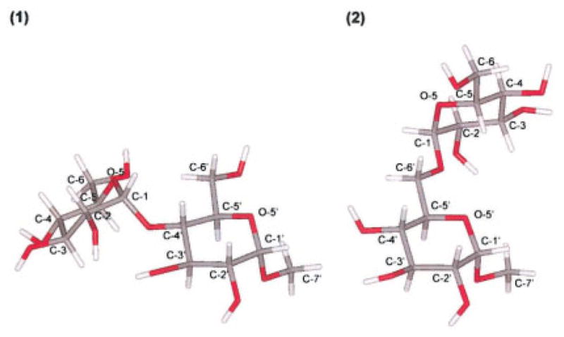
Molecular structure of compounds 1 and 2 including atomic labels. (1) methyl-α-D-maltoside, and (2) methyl-α-D-isomaltoside.

MATERIALS AND METHODS

Nomenclature

Conformational flexibility around the glycosidic linkage α-(1→4) in compound 1 is described by the two torsional angles: Φ=O5–C1–O1–C4′ and Ψ=C1–O1–C4′–C5′ and by the three torsional angles in the case of the α-(1→6) linkage in compounds 2: Φ=O5–C1–O1–C6′, Ψ=C1–O1–C6′-C5′ and ω =O1–C6′–C5′–O5′. The orientation of the hydroxymethyl groups is given by Θ(O5–C5–C6–O6), the gauche conformers being denoted by the standard notation gg, gt, and tg (corresponding to angles of Θ of 300°, 60°, and 180°, respectively). The sign of the torsion angles is defined in agreement with the IUPAC Commission of Biochemical Nomenclature.²⁸

Synthesis

Methyl α-maltoside (1) and methyl α-isomaltoside (2) were obtained from methyl hepta-O-benzyl-α-D-maltoside (3) and methyl hepta-O-benzyl-α-D-isomaltoside (4), respectively, by the conventional catalytic hydrogenolysis procedure for O-debenzylation using 10% palladium on carbon. Compounds 3 and 4 were synthesized according to Garcia et al.²⁹ and references therein.

NMR Measurements

The samples were lyophilized three times against D₂O (98.6%) and dissolved oxygen was vacuum-removed prior to sealing in NMR tubes under argon. The NMR spectra were recorded on 60 and 65 mM solutions of methyl-O-α-D-maltoside and methyl-O--D-isomaltoside in 99.96% D₂O at 25°C. The chemical shift and homonuclear coupling constant data are listed in Table 1. ¹H chemical shift assignments were obtained from phase-sensitive DQCOSY spectra and carbon assignments were extracted from gHSQC and HMBC 2D spectra (Bruker Avance 500 and Varian INOVA 500 spectrometers). Homo- and heteronuclear coupling constants were measured at 500 MHz on Varian INOVA and Unityplus spectrometers. The digital resolution in the latter 1D spectra were 0.1 and 0.2 Hz/pt, respectively. The selective proton-detected heteronuclear long-range 1D coupling constant measurements from the Varian library were according to Blechta et al.³⁰ The raw data were multiplied by an exponential line-broadening factor of 0.5 prior to applying the Fourier transform. In some cases, band-selective homonuclear decoupling was implemented during acquisition to simplify the antiphase multiplet that contained the ³J_C,H values, thus increasing the accuracy of these data. The methylene proton resonating at low field in the vast majority of glucose derivatives is H6S, and it typically displays the smallest vicinal coupling to H5 (i.e., J_H5,H6R and J_H5,H6S are 5.5 and 2.4 Hz, respectively, in methyl α-glucoside^31–33). However, in 2 vicinal coupling of the low- (4.5 Hz) and highfield (2.0 Hz) prochiral H6′ methylene protons to H5′ of the methylated glucose residue showed the reverse pattern. Thus, a NOESY spectrum (500-ms mixing time) and intraresidue ³J_C4,H6 couplings were acquired to confirm the inversion in the chemical shifts of these proR and proS methylene protons using the approach described by Poppe in a study of gentiobiose.³⁴

Table 1.

¹H (500 MHz) and ¹³C (125 MHz) Chemical Shift and Homonuclear Coupling Constant Data for 60 mM Methyl-O-α-D-maltoside and 65 mM Methyl-O-α-D -isomaltoside Solutions in D₂O at 25°C.

Compound	H-1	H-2	H-3	H-4	H-5	H-6a,b
Sugar	(C-1)	(C-2)	(C-3)	(C-4)	(C-5)	(C-6)
Residue	3JH1,H2	3JH2,H3	3JH3,H4	3JH4,H5	3JH5,H6a 3JH5,H6b	3JH6a,H6b
Methyl-O-α-D-maltosidea
α-Glcp(1→4	5.317 (100.00) 3.9	3.491 (72.10) 9.8	3.603 (73.23) 8.2	3.333 (69.70) 9.8	3.630 (73.05) 1.8, 5.0	3.806, 3.725 (60.90b) 11.7
→4)-Me-O-α-Glcp	4.733 (99.46) 3.8	3.515 (71.41) 9.8	3.85 (73.92) 8.5	3.558 (77.18) 10.0	3.667 (70.46) 2.2, 5.0	3.775, 3.683 (60.84b) 11.7
Methyl-O-α-D- isomaltosidec
α-Glcp(1→6	4.866 (98.05) 3.7	3.468 (71.35) 9.8	3.637 (73.25) 9.2	3.340 (69.59) 9.8	3.630 (72.01) 2.3, 5.0	3.759, 3.677 (60.64) 12.2
→6)-Me-O-α-Glcp	4.731 (99.56) 3.8	3.484 (71.67) 9.8	3.571 (73.56) 9.0	3.429 (69.69) 10.1	3.740 (70.25) 4.5, 2.0	3.905, 3.653 (65.66) 11.3

H6a (H6b) designates the methylene proton that resonates at low field (high field).

^aOMe— −3.339, 55.6 ppm.

^bAssignments may be reversed.

^cOMe−03.339, 55.38 ppm.

Carbon T₁ and heteronuclear nOes were measured at 100.6 MHz (Bruker Avance 400 with either H/C z-gradient or QNP probes) with the inversion recovery and inverse-gated pulse sequences. The recycle times were between five and seven times the T₁ longest values. In the case of the T₁ measurements 12–15 spectra with delay times ranging from 0 to 2×T₁ were acquired. The values in Table 2 were obtained using the ratio of the integrals in the composite-pulse decoupled and inverse-gated spectra (sensitivity enhanced with line-broadening factors of 0.5 Hz). All relaxation experiments were repeated at least once. Translational self-diffusion coefficients were obtained as previously reported¹⁷ using the pulsed-field gradient stimulated spin-echo pulse sequence.³⁵

Table 2.

100.6 MHz Methine Carbon T₁ and Heteronuclear nOe Factor (η_CH) Data for 60 mM Methyl-O-α-D-maltoside and 65 mM Methyl-O-α-D-isomaltoside Solutions in D₂O at 25°C.

Compound	C1	C2	C3	C4	C5	Average Value
Sugar
Residue
Methyl-O-α-D-maltoside
α-Glcp(1→4	508 ±12 (1.65)	452 ±1 (1.48)	523 ±46 (1.48)	440 ±6 (1.38)	437 ±6 (1.57)	472 (1.51)
→4)-Me-O-α-Glcp	428 ±8 (1.76)	507 ±22 (1.63)	536 ±5 (1.42)	522 ±10 (1.37)	522 ±26 (1.32)	503 (1.50)
Methyl-O-α-D-isomaltoside
α-Glcp(1→6	496 ±23 (1.47)	507 ±21 (1.42)	457 ±21 (1.30)	465 ±18 (1.34)	451 ±20 (1.57)	475 (1.44)
→6)-Me-O-α-Glcp	508 ±17 (1.37)	465 ±24 (1.45)	476 ±19 (1.32)	465 ±26 (1.50)	487 ±22 (1.57)	480 (1.44)

A rough estimate of the overall tumbling time was extracted from a plot of the reciprocal of the average methine carbon T₁ value as a function of the theoretical spectral densities. These longitudinal relaxation times were homogeneous and showed typical average deviations (±5%). As the values of the heteronuclear nOes were also very uniform, it appears that overall motion is nearly isotropic. The standard deviations (~10–15%) of the heteronuclear nOes were much larger than for the T₁ data and these parameters were not used to estimate the global correlation time, τ_c.

Molecular Modeling

In the present investigation the aim was to investigate the force fields using simulation protocols that developers use. The simulation protocols may not be theoretically optimal, but have proven to give accurate results when applied to carbohydrates.

Constant nTP Molecular Dynamics Simulations Using AMBER

Simulations were performed by using the AMBER-6.0 program package²⁷ together with the GLYCAM-2000a parameters designed for carbohydrates.²⁶ The molecules were hydrated in the Xleap module of AMBER by a periodic box of TIP3P waters.³⁶ All the simulations were run with the SANDER module of AMBER with SHAKE algorithm³⁷ (tolerance =0.0005 Å) to constrain covalent bonds to hydrogens, using periodic boundary conditions, a 1-fs time step, a temperature of 300 K with Berendsen temperature coupling,³⁸ a 9-Å cutoff applied to the Lennard–Jones interactions, and constant pressure of 1 atm using isotropic position scaling.³⁸ The nonbonded list was updated every 10 steps. Scaling factors of 2.0 and 1.2 were used for 1–4 electrostatic and van der Waals interactions, respectively.

For both compounds, a periodic box of TIP3P waters was extended by 8 Å in each direction from the carbohydrate atoms to contain 578 water molecules in the case of compound 1 and 536 water molecules to solvate compound 2. Equilibration was performed by first restraining the atoms of the disaccharide (water molecules were allowed to move) and running 1000 iterations of energy minimization, of which the first 50 were made using the steepest descent method while subsequent iterations used the conjugated gradient method. After this initial minimization, all subsequent simulations were run by using the particle mesh Ewald method³⁹ with a cubic B-spline interpolation order and a 10⁻⁶ tolerance for the direct space sum cutoff. The first step was followed by 25 ps of dynamics with the position of the disaccharide fixed. At this point the density of the system reaches a value close to 1 g · cm⁻³. Equilibration was continued with 25 kcal · mol⁻¹ · Å⁻¹ restraints placed on all the solute atoms, minimization for 1000 steps, followed by 3 ps of molecular dynamics, which allowed the water to relax around the solute. This equilibration was followed by five rounds of 600 steps of minimization where the solute restraints were reduced by 5 kcal · mol⁻¹ · Å⁻¹ during each round. Finally, the system was heated from 100 to 300 K over 20 ps and the production run was initiated. Initial velocity for all atoms was assigned from a Boltzmann distribution at 300 K. Trajectory coordinates were sampled for 10 ns, with a spacing of 40 fs.

Constant nTV Molecular Dynamics Simulations Using CHARMM

Microcanonical molecular dynamics simulations at 300 K were performed using the CHARMM program package, together with HGFB or CSFF force field. The water molecules of the solvent were modeled using the TIP3P potential energy function.³⁶ In the simulation, Newton’s equations of motion were integrated for each atom using the two-step velocity Verlet algorithm⁴⁰ with a 1-fs time step. All hydrogen atoms were explicitly included in the simulations, although bond lengths involving hydrogen atoms were kept fixed throughout the simulation using the constraint algorithm SHAKE. Minimum convention boundary conditions were used during the simulations, and interactions between atoms more than 12 Å apart were truncated and switching functions were used to smoothly turn off long-range interactions between 10 and 11 Å. The nonbonded list was updated every 10 steps.

For both compounds, the coordinates of the starting conformation were superimposed upon the coordinates of a well-equilibrated (at 300 K) box of 512 water molecules. In the case of compound 1, this procedure left 490 water molecules in the primary box when deleting those water molecules, whose van der Waals radii overlapped with any of the atoms of the solute. In the case of compound 2, 492 water molecules were left in the periodic box. After this virtual solvation, the system was energy minimized with 50 steepest descent iterations with the original box size to relax steric conflicts that might have been created in the generation of the box and to relax the solute structure in the new environment. Then the cubic box length was slightly adjusted to give a density of 1.00 g · cm⁻³. Initial velocity for all atoms was assigned from a Boltzmann distribution at 300 K. The system was equilibrated for 100 ps to relax any artificial starting conditions produced by the solvation procedure, with occasional scaling of the atomic velocities when the average temperature deviated from the desired temperature of 300 K by more than an acceptable tolerance of ±3 K. Following the equilibration period, the Verlet integration was continued without any further interference for a subsequent 10 ns. Complete phase points were saved every 20 fs for later analysis.

Calculation of Homo- and Heteronuclear Coupling Constants

³J coupling constants were calculated from the trajectories, utilizing the dependence of molecular dihedral structure on vicinal coupling constants through the Karplus relationship⁴¹ by averaging all frames in the trajectories. In this work the heteronuclear coupling constants ³J_C,H were calculated using the Karplus-type equation for the C–O–C–H segment parametrized by Tvaroska et al.,^{42 and 3}J_H,H homonuclear coupling constants were calculated using the parametrization by Stenutz et al.⁴³

RESULTS AND DISCUSSIONS

Solute Geometry and NMR Coupling Constants

Methyl-α-D-maltoside

Figure 2A shows the MM3⁴⁴ potential energy surface in (Φ, Ψ)-space in vacuum of α-maltose adapted from Dowd et al.⁴⁵ This map exhibits two major minima, of which only the upper large energy minimum well is populated. This potential energy well can be subdivided into three minima. (1) The global minimum B (Φ=100°, Ψ=223°), which encompasses the crystal structure of α-maltose⁴⁶ (Φ=116, Ψ=242°) favored by an intramolecular hydrogen bond between O-2…O-3′; (2) minimum A (Φ=68°, Ψ=198°), which is similar in energy to minimum B, but does not promote the above mentioned intramolecular hydrogen bond; and (3) minimum C (Φ=153°, Ψ=260°), which is higher in energy but, like minimum B, allows for an intramolecular O-2…O-3′ hydrogen bond.

Figure 2.

Population density maps and MM3-generated relaxed-residue steric energy maps. (A) The adiabatic map of α-maltose as a function of Φ and Ψ. Isoenergy contours are drawn at 1 kcal · mol⁻¹ increments to 8 kcal · mol⁻¹ above the global minimum. (B) Population density maps of methyl-α-D-maltoside in aqueous solution as a function of Φ and Ψ calculated from the three trajectories. Contours are drawn at (0.1, 0.01, 0.001, and 0.0001) population levels. All three figures have been superimposed on the outer contour of the MM3 energy maps of α-maltose. (C) Adiabatic maps of α-isomaltose as a function of Φ and Ψ and three staggered ω conformations. Isoenergy contours are drawn at 1 kcal · mol⁻¹ increments to 8 kcal · mol⁻¹ above the global minimum. (D) Population density maps of methyl-α-D-isomaltoside in aqueous solution as a function of Φ and Ψ calculated from the three trajectories. Contours are drawn at (0.1, 0.01, 0.001, and 0.0001) population levels. All three figures have been superimposed on the outer contour of the MM3 energy maps of α-isomaltose. (E) Population density maps of methyl-α-D-isomaltoside in aqueous solution as a function of Ψ and ω calculated from the three trajectories. Contours are drawn at (0.1, 0.01, 0.001, and 0.0001) population levels. All three figures have been superimposed on the outer contour of the corresponding MM3 energy maps. All figures include positions of the global minimum (+).

The methyl-α-D-maltoside trajectories (Table 3) were all initiated from the conformation found in the crystal structure of α-maltose⁴⁶ corresponding to minimum B. Figure 2B (left) shows the population density map of the 10-ns trajectory carried out using the HBFG force field (denoted T1–CH). As indicated by the figure, there is a shift away from minimum B towards minimum A with a peak density at (Φ = 61°, Ψ = 191°) and average density at (〈Φ〉 = 66°, 〈Ψ〉 = 199°). It is characteristic of this trajectory that the intramolecular hydrogen bond between O-2…O-3′ occurs only about 11% of the time (distance O…O ≤ 3.3 Å). In T1–CH the hydroxyl groups apparently prefer to form intermolecular hydrogen bonds with the water molecules, and thus the intramolecular hydrogen bond contributes little to the stabilization of glycosidic linkage conformation. The trajectory calculated in the present work matches the gross features of previous MD studies on maltose in solution in which mainly the A well is populated and only occasionally the B well.^47–51 The absence of the O-2…O-3′ intramolecular hydrogen bond in water is in agreement with experimental studies on maltose.^52–55

Table 3.

Details about the Different MD Simulations Carried Out in This Work.

Compound	HGFB	CSFF	Amber
Me-α-D-maltoside (1)	T1—CH (490)	T1—CSFF (490)	T1—AMB (578)
Me-α-D-isomaltoside (2)	T2—CH (492)	T2—CSFF (490)	T2—AMB (536)

The number of TIP3P water molecules used in each calculation is given in parentheses. The time recorded for each trajectory was 10 ns.

The 10 ns trajectory recorded in the CSFF force field, denoted T1–CSFF, displays a different population distribution map (Fig. 2B, middle) from that of the older force field. In this case, that minimum at B continues to be significantly populated and the intramolecular hydrogen bond between O-2 and O-3′ occurs about 27% of the time. The relatively high occurrence of this intramolecular hydrogen bond has also been reported in recent theoretical studies of the aqueous solution for α-maltose,⁵⁶ α-panose, and for the tetrasaccharide α-D-glucosylmaltotriose.¹⁶ Figure 2B (right) shows the result of the 10-ns trajectory carried out using the GLYCAM force field (denoted T1–AMB). In this case, the maltoside resides most of the time in the global minimum B and the intramolecular hydrogen bond between O-2…O-3′ persists about 30% of the time. This result is in agreement with Brady and Schmidt,⁴⁷ who reported the presence of this hydrogen bond for β-maltose in aqueous solution using a CHARMM-type force field.⁴⁸ The average values of the torsion angles Φ and Ψ obtained from T1–CH, T1–CSFF, and T1–AMB were (〈Φ〉=66°, 〈Ψ〉=199°), (〈Φ〉=80°, 〈Ψ〉=212°), and (〈Φ〉=86°, 〈Ψ〉=224°), respectively.

In this study, we measured the two heteronuclear coupling constants across the glycosidic linkage of the methyl α-D-maltoside: ³J_C-4′,H-1 and ³J_C-1,H-4′ to 4.1 and 4.9 Hz, respectively, which is in relatively good agreement with the values measured on methyl β-D-maltoside by Perez et al.⁵² (³J_C4′–H1 = 4.0, ³J_C1–H4′ = 4.5 Hz). The ensemble averaged calculated coupling constants are listed in Table 4. As observed from the table, the calculated coupling constants obtained with the GLYCAM-2000a force fields are almost in perfect agreement with the experimental coupling constants, whereas the two CHARMM based force fields fail to model the dihedral behavior correctly. However, the calculated values obtained using the CSFF force field were considerably better than those obtained using the HBFG force field.

Table 4.

Measured and Calculated ³J Coupling Constants (Hz) of Compounds 1 and 2.

	3JC4′—H1 (ϕ)	3JC1—H4′ (φ)	3JC6′ —H1 (ϕ)	3JC1—H6′R (φ)	3JC1—H6′S (φ)	3JH5—H6R (ω)	3JH5′ H6S (ω)	3JH5′ —H6′R (ω)	3JH5′ —H6′S (ω)	3JC1′ —CH3
(1)	4.1	4.9	—	—	—	5.0	1.8	5.0	2.2	4.4
T1—CH	1.88	2.92	—	—	—	4.13	6.45	3.40	4.07	3.34
T1—CSFF	3.38	3.92	—	—	—	4.09	2.77	2.07	2.02	3.34
T1—AMB	3.99	4.88	—	—	—	5.82	2.01	2.26	1.72	3.34
(2)a	—	—	3.2	3.3a	3.8a	5.0	2.3	4.5	2.0	4.2
T2—CH	—	—	2.45	2.37	2.05	4.48	7.27	3.52	4.51	3.34
T2—CSFF	—	—	2.68	3.10	2.00	3.76	2.79	9.30	1.42	3.34
T2—AMB	—	—	2.44	2.75	2.00	6.47	1.92	5.65	1.88	3.36

Heteronuclear coupling constants (Hz) of 60 mM methyl-O-α-D-maltoside and 65 mM methyl-O-α-D-isomaltoside solutions in D₂O at 25°C.

^aStereospecific assignments were established with the approach used for gentiobiose;³⁴ homonuclear nOes (a_ij) for the methylated glucose—a_H5′,H6′S > a_H5′,H6′R, and a_H4′,H6′S <a_H4′,H6′R; terminal glucose—³J_C4,H6S = 3.5 Hz.

Methyl-α-D-isomaltoside

The starting conformation in compound 2 was taken as the geometry of the α(1→6) linkage found in the crystal structure of α-panose⁵⁷ (Φ = 71°, Ψ = 165°, ω= 75°). Compared to 1, methyl-α-D-isomaltose is much more flexible due to the three-bond glycosidic linkage. Figure 2C displays the MM3 adiabatic maps obtained for α-isomaltose as a function of Φ, Ψ dihedrals for the three staggered orientations of ω, 300° (gg), 60° (gt), and 180° (tg), presented here in order of increasing energy.⁵⁸ All the wells have Φ in the proximity of 80° in accordance with the exoanomeric effect and Ψ has a value of 180° in the three lowest energy conformations. Figures 2D and 2E displays the population density maps for the α-(1→6) linkage obtained in the three trajectories. From the plots two observations are readily made: the geometry of the crystal conformation of panose is nearly perfect, centered in the most populated region, and Φ appears to be the most constrained parameter, in good agreement with the exoanomeric effect. While the Ψ dihedral takes an average value around 180° in T2–CH and T2–AMB, it is more flexible in trajectory T2–CSFF, in which it adopts two different values centered around Ψ=60 and Ψ=180. This double-well characteristic of the Ψ dihedral has been previously reported by Naidoo et al.¹⁵ for β-isomaltose, α-panose, and α-D-glucosylmaltotriose¹⁶ using the force field developed by Palma et al.⁵⁹ The authors explain the frequent transitions of the Ψ dihedral for the tri- and tetrasaccharides by hypothesizing that the addition of an extra residue provides alternative interactions on either side of the branch point increasing its flexibility. Concerning the ω-dihedral, which together with the Φ-dihedral (restricted by the exoanomeric effect) is the least flexible dihedral angle present in the simulations, transitions are observed between all three possible staggered conformers (gg, gt, and tg) in T2–CH (see Fig. 3). This fact indicates that the energy difference between the three minima wells (gg, gt, and tg) in the HBFG force field is relatively low, giving a quite flexible system. However, the presence of a tg conformation has not been experimentally observed in α-(1→6) linked oligosaccharides.⁶⁰ The ratio between the three conformers gg:gt:tg obtained from HGFB was equal to 47:20:33. In T2–AMB, the ω torsion angle adopts mainly a gg or a gt conformation (gg:gt:tg = 43:56:1), whereas in trajectory T2–CSFF only the gt conformation is sampled. When starting the latter simulation in other geometries, the isomaltoside readily jumped back to the preferred gt ω-orientation.

Figure 3.

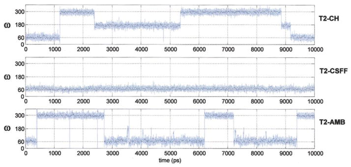
Time series monitoring the ω-dihedral in the 10 ns methyl-α-D-isomaltoside trajectories: T2–CH (HBFG), T2–CSFF (CSFF), and T2–AMB (GLYCAM-2000a). [Color figure can be viewed in the online issue, which is available at www.interscience.wiley.com.]

In contrast to the results for the methyl-α-D-maltoside, the measured and calculated heteronuclear coupling constants across the glycosidic linkage for the isomaltoside are not very conclusive. As can be observed from Table 4, the heteronuclear coupling constants calculated in the three trajectories are very similar, which is logical if we consider that the population of dihedrals Φ,Ψ is almost identical in all the simulations. Nevertheless, the values obtained with the CSFF force field are consistently closer to the experimental results, which could be related to a small population observed for dihedrals Φ,Ψ at (70, 70°) in this force field (Fig. 2).

Common Features

In all three trajectories of both compounds 1 and 2 the methyl group adopts a gt conformation most of the time in accordance with the exoanomeric effect. The gg conformation is not sampled due to steric interactions between the methyl group and the axial hydrogens of the ring. The heteronuclear coupling constant between C-1 and HMe measured in this work at 4.2–4.4 Hz is calculated to 3.3 Hz from all three trajectories, probably within the margins of uncertainty for this type of Karplus relationships.

In the case of the maltoside in the T1–CH trajectory, the hydroxymethyl groups visited all three staggered conformations with a ratio of gg:gt:tg = 22:21:57 and 48:23:29 for the nonreducing and reducing residue, respectively. In T1–AMB, the tg conformation was not sampled, yielding to gg:gt:tg ratios of 44: 56:0 and 85:15:0. Although the GLYCAM force field has been specially developed to obtain the correct rotamer population of ω dihedral,³ this particular rotamer distribution is a well-documented problem of the HBFG force field, which normally gives inconsistent primary alcohol sampling (tg > gt >gg) compared to that predicted by experiments (gg ≥ gt >tg).^{31–33,61,62} This peculiarity has been corrected in the new CSFF, which has been tested with β-glucose and β-galactose, and generates a rotamer population of primary alcohols that is in conformity with NMR data. In this maltoside study the T1–CSFF trajectory led to a gg:gt:tg ratio of 66:33:1 for the nonreducing residue and 88:12:0 for the reducing residue.

For compound 2, the overall picture of the conformational characteristics of the hydroxymethyl group remains inconsistent. In the T2–CH trajectory the hydroxymethyl group visits the three staggered conformations according to the ratio gg:gt:tg of 12:22: 66, which is in complete contrast to that obtained from the GLY-CAM trajectory T2–AMB (gg:gt:tg = 36:64:0). Also in the trajectory T2–CSFF (which exhibits considerably more transitions compared to the T2–AMB trajectory) the tg conformation is not sampled, but in this case the most stable hydroxymethyl rotamer is the gg conformation (gg:gt:tg =69:30:1).

The homonuclear ³J_H-5,H-6 coupling constants that probe the conformation of the hydroxymethyl group and the ω angle of the α(1–6) linkage display a remarkably constant pattern for these two model α-glucans (Table 4). Independent of the nature of the glucose unit, the maltoside and the participation in the glycosidic linkage the proR and proS coupling remains fairly constant near the values observed for α-D-glucose (approximately 5 and 2 Hz) as a monomer and in a range of different oligomeric compounds.^33,63 Not even the participation in the α(1–6) linkage perturbs the experimental ³J_H-5,H-6 values. In contrast, the theoretically derived coupling constant from the molecular dynamics trajectories displays large variations between the force fields used and between the positions of the C5–C6 groups in the α-glucan, with the values obtained with GLYCAM force field being closer to the experimental results (Table 4).

Solute Diffusion

The self-diffusion coefficients of methyl-α-D-maltoside 1 and methyl-α-D-isomaltoside 2 were obtained from a pulsed field gradient (PFG) NMR experiment¹⁷ yielding self-diffusion coefficients of 4.0 · 10⁻⁶ cm² · s⁻¹ and 4.2 ·10⁻⁶ cm² · s⁻¹, not significantly different from those of α-maltose⁴ and α-isomaltose (4.1¹⁷ and 3.8 10⁻⁶ cm² · s⁻¹, unpublished results, respectively). In comparison, the calculated self-diffusion obtained via the Stokes–Einstein relation and the center of mass mean-square displacement autocorrelation yielded a value of 3.8 ·10⁻⁶ cm² · s⁻¹ for trajectory T1–CH, 3.5 ·10⁻⁶ cm² · s⁻¹ for trajectory T1–CSFF, and 8.4 · 10⁻⁶ cm² · s⁻¹ for trajectory T1–AMB. Figure 4A shows the diffusion coefficient of compound 1 as a function of time for the three different trajectories. As previously experienced with sucrose and trehalose, the translational diffusion is modeled fairly well in the HBFG force field and also in the new generation force field CSFF. However, in T1–AMB the self-diffusion coefficient was calculated to be more than twice the experimental value, indicating a less structured carbohydrate–water system. However, in this context it should be emphasized that the self-diffusion coefficient for the TIP3P model employed in the simulations is almost twice the experimental value of pure water,⁶⁴ and thus can be expected to influence the disaccaride’s self-diffusion towards higher values.

Figure 4.

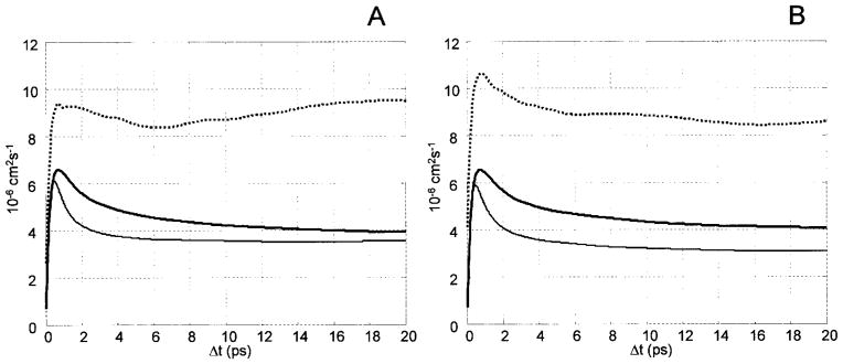
Calculated translational diffusion of (A) methyl-α-D-maltoside, and (B) methyl-α-D-isomaltoside. Thick line = HBFG, thin line =CSFF, and dotted line =GLYCAM-2000a.

Figure 4B shows the calculated translational diffusion of compound 2 as a function of time calculated for the three different trajectories. As for compound 1, the calculated value obtained from trajectory T2–CH (4.20 · 10⁻⁶ cm² · s⁻¹) conforms perfectly with the experimental observations, whereas the value calculated from trajectory T2–CSFF is a little lower and the value calculated from the T2–AMB trajectory is more than twice the experimental self-diffusion.

Rotational diffusion was assessed from the global correlation time: τ_c obtained from T₁ experiments and theoretically from the angular evolution of the solute dipole moment, as expressed by the autocorrelation function of the angular displacement of the dipole moment vector as a function of Δt. The autocorrelation function was subsequently fitted to a exponential relaxation function using the equation:

$$\mathbf{I}(\mathit{t})=\sum _{i=1}^N{M}_{0,i}·(1-2\times e^{(-\mathit{t}/T_{1,i})})$$

where t is the time displacement and T₁ the characteristic rotational diffusion coefficient. Interestingly, this quite labile approach (due to relatively short trajectories) led to a bi-exponential relaxation phenomenon: a relatively fast relaxation component (of typically 10 ps) dominating at short times and a slow relaxing component that represents the global molecular tumbling. In the case of methyl-α-D-maltoside this approach led to global autocorrelation times of approximately 160 ps for trajectory T1–CH, 140 ps for trajectory T1–CSFF, and 80 ps for trajectory T1–AMB. In the case of the methyl-α-D-isomaltoside, the corresponding values were 160 ps for T2–CH, 140 ps for T2–CSFF, and 80 ps for T2–AMB. In comparison, the experimental global correlation time was measured to be approximately 150 ps for both compounds. This may provide supporting evidence to the fact that the two CHARMM based force fields give more realistic solute–water interactions.

Isotropic Hydration

Detailed solute–solvent interactions were characterized by radial pair distribution functions (RPD). Figure 5 shows the RPD of water oxygen and a characteristic oxygen (O-3) of compound 1 (the corresponding RPDs of compound 2 are practically identical) in the three trajectories. The pair distribution obtained when using the HBFG force field displays a typical hydrophilic interaction with a well-defined first hydration shell with a density peak at 2.8 Å and a peak density of about 2.3, much like the corresponding interaction between water molecules (the experimental RPD for O…O interactions in water at 298 K is the gray shadow⁶⁵). In comparison, the RDP calculated when using CSFF force field displays a density at 2.8 Å of only 1.6, in agreement with the value calculated by Naidoo and Kuttel⁵⁶ for β-maltose using the same force field. In contrast, the RDP calculated from the GLYCAM 2000a force field has a peak at about 3.0 Å with a peak density of only 1.0 and no well-defined secondary hydration shell. It is beyond the scope of this investigation to provide experimental evidence for such RDPs, but the mean O…Ow distance for carbohydrates in crystals is 2.77 Å⁶⁶ and the distance between O…Ow found in the crystal structure of β-maltose monohydrate is 2.8 Å.⁶⁷

Figure 5.

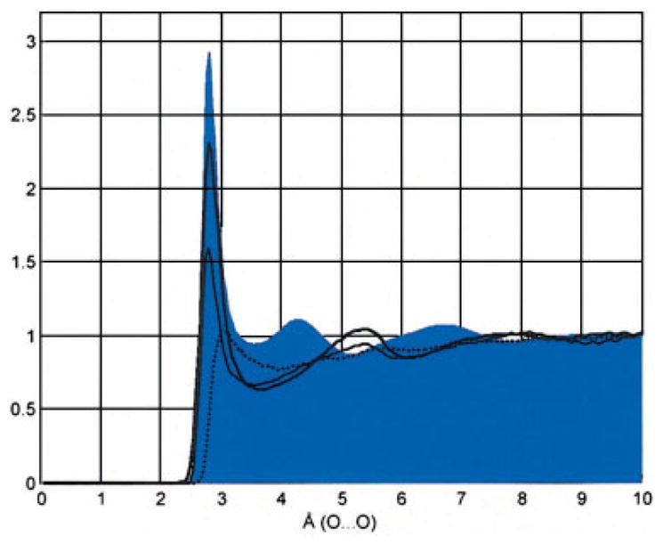
Radial pair distribution function (RPD) of water and oxygen O-3 of methyl-α-D-maltoside. Thick line = HBFG, thin line = CSFF, and dotted line =GLYCAM-2000a. The gray background contour is the experimental Ow…Ow radial pair distribution of water. [Color figure can be viewed in the online issue, which is available at www.interscience.wiley.com.]

To further assess this fundamental property of the carbohydrate–water interaction we estimated the dimerization energy of methanol using the carbohydrate parameters of the three force fields. In CSFF and HBFG, the energy and the geometry of the optimized methanol dimer is quite close to that calculated with quantum mechanics⁶⁸ (Table 5). The same calculation using GLY-CAM-2000a yielded a similar energy of −4.48 kcal · mol⁻¹ at a much longer O…O distance. In comparison, the OPLS force field⁶⁹ developed to be able to reproduce experimental pure liquid properties and the free energies of solvation yields an O…O distance similar to the CHARMM force fields, but with a higher interaction energy. The pairwise additive approximation makes it necessary to have about 10–20% larger interaction energies and shorter interatomic distances in comparison to the ab initio gas phase dimers. The most significant difference between the three force fields is the Van der Waals radii of the hydroxyl oxygens, which for the GLYCAM force field has a value of 1.96 Å to be compared with 1.77 Å for CSFF and 1.60 Å for the HBFG force field.

Table 5.

Calculated Dimerization Energy of Methanol and Equilibrium Distances between the Two Oxygens in the Optimized Geometry.

Method	Δ Edimer kcal · mol−1	Rdimer Å
CSFF	−4.38	2.82
HGFB	−4.48	2.85
GLYCAM-2000a	−4.48	3.16
OPLS	−5.63	2.81
QM76}	−5.44	2.89
QM (H2O)77}	−5.00	2.90
Experimental78}		~2.92

To compare the solvent structure around compounds 1 and 2 with that of previous molecular dynamics studies conducted for the nonreducing disaccharides sucrose⁷⁰ and trehalose⁷¹ in the HBFG force field a principal component analysis (PCA)⁷² of the O…Ow RPDs was carried out. The result of the PCA is shown in Figure 6 and displays a clear clustering into three groups. Interestingly, 95% of the variation in the RPDs can be described by only two principal components (PCs), which represent the first hydration shell (peak at 2.8 Å) and the secondary hydration shell (peak at 4.4 Å), respectively, and moreover, this result suggests that the presence of a first hydration shell does not necessarily imply a secondary hydration shell. On the left side of the PC1 axis (describing the largest variation, which in this case is the magnitude of the first hydration shell) we find the ether and methyl oxygens that can act only as hydrogen bond acceptors and which are largely devoid of a primary hydration shell. On the right side of the PC1 axis we find a large cluster of hydroxyl oxygens that can act both as hydrogen bond acceptors and donors and that possess a highly populated primary hydration shell. PC2, which primarily characterizes the magnitude of the secondary hydration shell, divides the ether oxygens into methyl oxygens and ring and glycosidic oxygens, the methyl oxygens having a more well-defined secondary hydration shell. It is also observed (along PC1) that the ring oxygens (O-5) are consistently better hydrated than the glycosidic oxygens (O-1) and that O1g in the less compact α(1–6)-linkage of compound 2 is the better hydrated of the glycosidic oxygens.

Figure 6.

PCA on RPD of all oxygens of methyl-α-maltoside (■ black), methyl-α-isomaltoside (◆ black), trehalose (☆ blue), and sucrose (◆ red). [Color figure can be viewed in the online issue, which is available at www.interscience.wiley.com.]

Upon scrutinizing the large cluster of hydroxyl oxygens we observe that O-2, O-3, and O-6 are placed towards the right of PC1 with large magnitudes of the first hydration shell, and that O-4 tends to be less hydrated. Along the PC2 axis it is observed that the O-6 oxygen atoms of the more accessible primary hydroxyl groups have more water density at 4.4 Å, while the O-2 oxygen atoms have less. The two hydroxyl oxygens, O-3f of sucrose and O-4′ of methyl-α-D-isomaltose, are extremes. We have previously discussed the fructosyl O-3f of sucrose that is particular in several aspects, as it interacts in a cooperative water bridge between O-1f of the fructofuranosyl ring and O-2g of the glucose ring. It has particularly long water residence times (2.3 ps), which may indicate that it acts as a fixed point with respect to the water structure.¹⁴ Of greater interest to this study is the outlying position of O-4′ of compound 2 and the relatively extreme positions of O-3′ and O-6′ of compound 1. Oxygen O3′ in compound 1 exhibits a significant lack of water structure due to its participation in the most populated intramolecular hydrogen bond in which it acts as donor most of the time. Oxygen O-6′ in 1 is not involved in any significant intramolecular hydrogen bond, but participates in a water bridge to O-6. Last, but not least, O-4′ of 2 is active in two intraring water bridges to O-6 and O-2 (vide infra).

Table 6 shows the calculated hydration numbers of the two maltoside compounds as given by the average number of water molecules in strong interaction with the solute (less than 2.8 Å form the solute oxygens). At first observation the calculated hydration numbers are quite similar, but large differences are found amongst the three force fields. For example, trajectory T1–CH revealed an average hydration number of seven water molecules per methyl-α-D-maltoside molecule (Table 6), a value that decreases to 4.8 in the case of the T1–CSFF trajectory and to only 0.5 in the T1–AMB. Besides being temperature and concentration dependent, hydration numbers are also dependent on the experimental technique applied.⁷³ In the case of α-D-maltose, the hydration number has been determined experimentally by differential scanning calorimetry to 2.4–4,⁵⁰ by ultrasonic measurements to 14.1 and by quasielastic neutron scattering to 8.4.⁷⁴

Table 6.

Calculated Hydration Numbers of Compounds 1 and 2.

	Methyl-α-D-maltoside (1)		Methyl-α-D-isomaltoside (2)
	r < 3.5 Å	r <2.8 Å	R <3.5 Å	r <2.8 Å
T—CH	24.9	7.0	25.5	7.2
T—CSFF	19.1	4.8	20.1	4.9
T—AMB	17.4	0.5	18.3	0.6

Anisotropic Hydration

In this study we use normalized two-dimensional radial pair distributions⁷⁵ to quantify the magnitude of the localized water density. Figure 7 displays the maximum magnitude of all the shared water densities (Os…Ow…Os) for compounds 1 and 2 in the first hydration shell. Again the highest shared densities are obtained when the old CHARMM-type force field is used, and for both compounds the highest shared water density is observed between the two neighboring intraring hydroxyl groups rather than interring hydroxyl groups. Only in the HBFG force field we observe the existence of interring water bridges. The most significant interring water bridge found in compound 1 (Fig. 7A) is the one between the two primary hydroxyl groups (O-6…Ow…O-6′). In the methyl-α-D-isomaltoside (Fig. 7B) we observe three interring water bridges. Curiously, the behavior of O-4′ is quite similar to that exhibited by oxygen O-3f in sucrose⁷⁰ and most likely the reason why it was outlying in the PCA described in the previous section. In sucrose, O-3f and O-1f participates in a significant interresidue water bridge with O-2g. In compound 2, O4′ participates in two water bridges, one between O-6 and O-4′, with a maximum density of 3.3 obtained from HGFB force field, and another one between O-2 and O-4′. The last one, which has an average maximum density of 3.6 throughout the whole trajectory, is present only when ω dihedral adopts a gt conformation. The most significant localized water density site for compound 2 was found between O-2 and O-5′, which have previously been reported for isomaltose.¹⁵ The high water density around these two oxygens was about 4.8 times the bulk density in T2–CH, creating an interresidue water bridge.

Figure 7.

Maximum shared water densities among (A) methyl-α-D-maltoside, and (B) methyl-α-D-isomaltoside oxygens as calculated by normalized 2D pair distribution functions at Os…Ow distance between 2.8–3.5 Å. Densities crossing the glycosidic linkages are indicated with dashed lines. Normal = CSFF, bold =HGFB, and italic =GLYCAM-2000a. [Color figure can be viewed in the online issue, which is available at www.interscience.wiley.com.]

Figure 8A shows the normalized 2D radial pair distribution of water for compound 1 in which neighboring atoms O-4 and O-3 are the reference sites. In HGFB, the contour plot is highly symmetric and the peak is situated at about (2.8, 2.8 Å). The magnitude of the shared water density is about 6.4 times the bulk water density. Curiously, in CSFF force field an asymmetric situation is obtained. The fact that the peak (with a magnitude of 2.0 times the bulk density) is moved upward to (2.8, 3.3 Å) suggests that such a situation is sterically restricted, being the shared water molecule closer to atom O-4. Based on the RDPs calculated previously from GLYCAM, it is not surprising to find a shared water density around the two neighboring hydroxyl groups about only 1.2 times the bulk density and a peak situated at about (3.0, 3.0 Å).

Figure 8.

Two-dimensional radial pair distribution functions of different bridging water situations of methyl-α-D-maltoside. Isocontours: 0.96, 1.2, 2.0, 3.0, 4.0, 5.0, 6.0, and 7.0 cal · mol⁻¹. [Color figure can be viewed in the online issue, which is available at www.interscience.wiley.com.]

The most significant interring water bridge found in compound 1, in which atoms O-6 and O-6′ are the reference sites, is shown in Figure 8B. The maximum density of the shared water was calculated to 4.4 in T1–CH, but only to 1.4 in T1–CSFF and T1–AMB. Again, an asymmetric situation was found in CSFF as well as in GLYCAM. An additional weak localized water density site is present between O-2 and O-3′(Figure 8C). In this case the water density between the two oxygens is approximately 2.9 in T1–CH, 1.4 in T1–CSFF, and 1.4 in T1–AMB.

The interring water density values obtained using the HBFG force field are different from those calculated previously for sucrose and trehalose, supporting the hypothesis that all carbohydrates are hydrated uniquely. Although sucrose exhibits an extremely strong and sharp shared water density with a peak maximum of approximately nine times the bulk density between O-2g and O-1f, the maximum two-dimensional RDP density of an interring shared water in trehalose⁷¹ was calculated for O-2…O-4′ to be 2.4. This value is comparable in level to the maximum water density in the one-dimensional RDP, that is, trehalose is isotropically hydrated.

Conclusions

The conclusions of this study are twofold: (1) the internal motions of the solute, and (2) the solute–-water interactions.

Ad. I

With the precaution that the average J-couplings are not fully converged with the 10-ns simulations presented here it would appear from the heteronuclear coupling constants that in the case of the α(1→4) linkage the new generations of force fields give much better reproduction of the most important molecular degree of flexibility, namely the glycosidic linkage. The GLYCAM force field is near perfect. Regarding the α(1→6) linkage, the situation is not very obvious, but it would appear as if none of the force fields are sufficiently balanced to model the delicate interactions between intramolecular and intermolecular forces of this flexible and accommodating linkage. Exactly the same conclusion can be reached when discussing the reproduction of the primary hydroxyl rotamers and related homonuclear coupling constants. Although it is well known that these sensitive conformational parameters are poorly reproduced in the HBFG force field, the agreement with the experimental data of the two new generation force fields was disappointing. Worst is the fact that the relatively low variation of the homonuclear H5–H6 coupling constants (independent of position and participation in the glycosidic linkage) is not reflected in the theoretical models. The extent to which we can attribute discrepancy to the crude Karplus equation approach remains to be elucidated (this becomes a secondary remaining question).

Ad. II

Solute–water interactions were investigated from several angles: (1) 1D and 2D radial pair distributions scrutinizing localized carbohydrate-water interactions, (2) the translational diffusion of the solute, and (3) the rotational diffusion of the solute.

The radial pair distribution functions between water oxygens and the hydroxyl oxygens of the solute best resemble the RPD of water–water interactions when the HBFG force field is applied. It provides the most structured water–solute system, giving a density of at least 2.3 times the bulk water density in the first hydration shell. This hydration property of HGFB force field appears to lead to better reproduction of experimental translational and rotational diffusion coefficients than both of the new force fields. Along with simple calculations on the methanol dimer, circumstantial evidence is accumulating to support the validity of this more structured carbohydrate–water model. The low water density obtained for the first hydration shell for GLYCAM was only about the level of bulk water density that led to very low hydration numbers (only 0.5 water molecules in methyl-α-D-maltoside) in comparison to 7.0 obtained in the old CHARMM-type force field. In CSFF, the water density observed in the first hydration shell was calculated to 1.6 and the hydration numbers, as well as the translational diffusion coefficients, were slightly lower than those obtained with the HGFB force field.

Although all three force fields agree that intramolecular interring hydrogen bonds contribute little (less than 30%) to the stabilization of glycosidic linkage conformation of the two compounds, the simulations carried out in the old CHARMM-type force field suggest that the interresidue water bridges found in both compounds contribute to stabilize the structures in water solution. Moreover, the interring water density values obtained using the HBFG force field are different from those calculated previously for sucrose and trehalose, supporting the hypothesis that all carbohydrates are hydrated uniquely.

The preferred conformation for each of the two model compounds of amylopectin studied in this work, methyl-α-D-maltoside and methyl-α-D-isomaltoside, appears to be significantly influenced by water. The study reveals that especially the α-(1→6) glycosidic linkage is to some extent flexible in aqueous solution, exhibiting transitions of the ω dihedral throughout the simulations. The old CHARMM-type force field (HGFB) suggests an important population of the tg conformer when the α-(1→6) linkage was simulated, which is not in accordance with experimental data. This situation has been notably improved in the new force fields where GLYCAM presents the more flexible structure for the α-(1→6) linkage exhibiting transitions for ω dihedral between the gg and gt conformers throughout the simulation. In contrast, in the CFSS trajectory only the gt conformer was present.

This study indicates that future carbohydrate force field developments should emphasize and integrate carbohydrate–water interactions. Before this is possible, high-level ab initio calculations and advanced experiments (light scattering) are required to further establish the nature and magnitude of these basic intermolecular interactions. Only when such data have been collected will it be possible to evaluate whether a more appropriate modeling of the charge density (including lone pairs and perhaps also multipole charges and polarizabilities) is required to provide fully satisfactory models.

References

- 1.Brady JW. J Am Chem Soc. 1989;111:5155. [Google Scholar]
- 2.Engelsen SB, Hervé du Penhoat C, Pérez S. J Phys Chem. 1995;99:13334. [Google Scholar]
- 3.Kirschner KN, Woods RJ. Proc Natl Acad Sci USA. 2001;98:10541. doi: 10.1073/pnas.191362798. [DOI] [PMC free article] [PubMed] [Google Scholar]
- 4.Engelsen SB, Monteiro C, Hervé du Penhoat C, Pérez S. Biophys Chem. 2001;93:103. doi: 10.1016/s0301-4622(01)00215-0. [DOI] [PubMed] [Google Scholar]
- 5.Di Bari M, Cavatorta F, Deriu A, Albanese G. Biophys J. 2001;81:1190. doi: 10.1016/S0006-3495(01)75776-1. [DOI] [PMC free article] [PubMed] [Google Scholar]
- 6.Franks F. In: In Water Relationships in Food. Levine H, Slade L, editors. Plenum Press; New York: 1991. p. 1. [Google Scholar]
- 7.Duus JØ, Gotfredsen CH, Bock K. Chem Rev. 2000;100:4589. doi: 10.1021/cr990302n. [DOI] [PubMed] [Google Scholar]
- 8.Jeffrey GA. Acta Crystallogr B Struct Sci. 1990;46:89. doi: 10.1107/s0108768189012449. [DOI] [PubMed] [Google Scholar]
- 9.Pérez S. Methods Enzymol. 1991;203:510. doi: 10.1016/0076-6879(91)03029-g. [DOI] [PubMed] [Google Scholar]
- 10.Stroyan EP, Stevens ES. Carbohydr Res. 2000;327:447. doi: 10.1016/s0008-6215(00)00072-0. [DOI] [PubMed] [Google Scholar]
- 11.Kacuráková M, Wilson RH. Carbohydr Polym. 2001;44:291. [Google Scholar]
- 12.Mathlouthi M, Koenig JL. Adv Carbohydr Chem Biochem. 1986;44:7. doi: 10.1016/s0065-2318(08)60077-3. [DOI] [PubMed] [Google Scholar]
- 13.Imberty A, Pérez S. Chem Rev. 2000;100:4567. doi: 10.1021/cr990343j. [DOI] [PubMed] [Google Scholar]
- 14.Engelsen SB. In: In Water in Biomaterials Surface Science. Morra M, editor. John Wiley and Sons; Chichester, UK: 2001. p. 53. [Google Scholar]
- 15.Best RB, Jackson GE, Naidoo KJ. J Phys Chem B. 2001;105:4742. [Google Scholar]
- 16.Best RB, Jackson GE, Naidoo KJ. J Phys Chem B. 2002;106:5091. [Google Scholar]
- 17.Monteiro C, Hervé du Penhoat C. J Phys Chem A. 2001;105:9827. [Google Scholar]
- 18.Diaz MD, Berger S. Carbohydr Res. 2000;329:1. doi: 10.1016/s0008-6215(00)00239-1. [DOI] [PubMed] [Google Scholar]
- 19.Hamelin B, Jullien L, Derouet C, Hervé du Penhoat C, Berthault P. J Am Chem Soc. 1998;120:8838. [Google Scholar]
- 20.Rampp M, Buttersack C, Lüdemann HD. Carbohydr Res. 2000;328:561. doi: 10.1016/s0008-6215(00)00141-5. [DOI] [PubMed] [Google Scholar]
- 21.Petrova P, Monteiro C, Koca J, Hervé du Penhoat C, Imberty A. Biopolymers. 2001;58:617. doi: 10.1002/1097-0282(200106)58:7<617::AID-BIP1035>3.0.CO;2-1. [DOI] [PubMed] [Google Scholar]
- 22.Pérez S, Imberty A, Engelsen SB, Gruza J, Mazeau K, Jiménez–Barbero J, Poveda A, Espinoza JF, van Eijck BP, Johnson G, French AD, Kouwijzer MLCE, Grootenhuis PDJ, Bernardi A, Raimondi L, Senderowitz H, Durier V, Vergoten G, Rasmussen K. Carbohydr Res. 1998;314:141. [Google Scholar]
- 23.Brooks BR, Bruccoleri RE, Olafson BD, States DJ, Swaminathan S, Karplus M. J Comput Chem. 1983;4:187. [Google Scholar]
- 24.Ha SN, Giammona A, Field M, Brady JW. Carbohydr Res. 1988;180:207. doi: 10.1016/0008-6215(88)80078-8. [DOI] [PubMed] [Google Scholar]
- 25.Kuttel M, Brady JW, Naidoo KJ. J Comput Chem. 2002;23:1236. doi: 10.1002/jcc.10119. [DOI] [PubMed] [Google Scholar]
- 26.Woods RJ, Dwek RA, Edge CJ, Fraser–Reid B. J Phys Chem. 1995;99:3832. [Google Scholar]
- 27.Case DA, Pearlman DA, Caldwell JW, Cheatham TE, Ross WS, Simmerling CL, Darden TA, Merz KM, Stanton RV, Cheng AL, Vicent JJ, Crowley M, Tsui V, Radmer RJ, Duan Y, Pitera J, Massova I, Seibel GL, Singh UC, Weiner PK, Kollman PA. AMBER 6.0. University of California; San Francisco: 1999. [Google Scholar]
- 28.IUPAC-IUB. Carbohydr Res. 1997;297:1. doi: 10.1016/s0008-6215(97)83449-0. [DOI] [PubMed] [Google Scholar]
- 29.Garcia BA, Poole JL, Gin DY. J Am Chem Soc. 1997;119:7597. [Google Scholar]
- 30.Blechta V, del Rio-Portilla F, Freeman RJ. Magn Reson Chem. 1994;32:134. [Google Scholar]
- 31.Nishida Y, Ohrui H, Meguro H. Tetrahedron Lett. 1984;25:1575. [Google Scholar]
- 32.Ohrui H, Nishida Y, Watanabe M, Hori H, Meguro H. Tetrahedron Lett. 1985;26:3251. [Google Scholar]
- 33.Bock K, Duus JØ. Carbohydr Chem. 1994;13:513. [Google Scholar]
- 34.Poppe L. J Am Chem Soc. 1993;115:8421. [Google Scholar]
- 35.Tanner JE. J Chem Phys. 1970;52:2523. [Google Scholar]
- 36.Jorgensen WL. J Am Chem Soc. 1981;103:335. [Google Scholar]
- 37.Ryckaert JP, Ciccotti G, Berendsen HJC. J Comput Phys. 1977;23:327. [Google Scholar]
- 38.Berendsen HJC, Postma JPM, van Gunsteren WF, Dinola A, Haak JR. J Chem Phys. 1984;81:3684. [Google Scholar]
- 39.Essmann U, Perera L, Berkowitz ML, Darden TA, Lee H, Pedersen LG. J Chem Phys. 1995;103:8577. [Google Scholar]
- 40.Verlet L. Phys Rev. 1967;159:98. [Google Scholar]
- 41.Karplus M. J Chem Phys. 1959;30:11. [Google Scholar]
- 42.Tvaroska I, Hricovini M, Petrakova E. Carbohydr Res. 1989;189:359. [Google Scholar]
- 43.Stenutz R, Carmichael I, Widmalm G, Serianni AS. J Org Chem. 2002;67:949. doi: 10.1021/jo010985i. [DOI] [PubMed] [Google Scholar]
- 44.Allinger NL, Rahman M, Lii JH. J Am Chem Soc. 1990;112:8293. [Google Scholar]
- 45.Dowd MK, Zeng J, French AD, Reilly PJ. Carbohydr Res. 1992;230:223. doi: 10.1016/0008-6215(92)84035-q. [DOI] [PubMed] [Google Scholar]
- 46.Takusagawa F, Jacobsen RA. Acta Crystallogr B Struct Sci. 1978;34:213. [Google Scholar]
- 47.Brady JW, Schmidt RK. J Phys Chem. 1993;97:958. [Google Scholar]
- 48.Ha SN, Madsen LJ, Brady JW. Biopolymers. 1988;27:1927. doi: 10.1002/bip.360271207. [DOI] [PubMed] [Google Scholar]
- 49.Astley T, Birch G, Drew MGB, Rodger PM. J Phys Chem A. 1999;103:5080. [Google Scholar]
- 50.Fringant C, Tvaroska I, Mazeau K, Rinaudo M, Desbrieres J. Carbohydr Res. 1995;278:27. doi: 10.1016/0008-6215(95)00232-1. [DOI] [PubMed] [Google Scholar]
- 51.Ott KH, Meyer B. Carbohydr Res. 1996;281:11. [Google Scholar]
- 52.Pérez S, Taravel FR, Vergelati C. New J Chem. 1985;9:561. [Google Scholar]
- 53.Stevens ES, Sathyanarayana BK. J Am Chem Soc. 1989;111:4149. [Google Scholar]
- 54.Lipkind GM, Verovsky VE, Kochetkov NK. Carbohydr Res. 1984;133:1. [Google Scholar]
- 55.Shashkov AS, Lipkind GM, Kochetkov NK. Carbohydr Res. 1986;147:175. doi: 10.1016/0008-6215(88)80156-3. [DOI] [PubMed] [Google Scholar]
- 56.Naidoo KJ, Kuttel M. J Comput Chem. 2001;22:445. doi: 10.1002/jcc.10119. [DOI] [PubMed] [Google Scholar]
- 57.Imberty A, Pérez S. Carbohydr Res. 1988;181:41. [Google Scholar]
- 58.Dowd MK, Reilly PJ, French AD. Biopolymers. 1994;34:625. doi: 10.1002/bip.360340505. [DOI] [PubMed] [Google Scholar]
- 59.Palma R, Himmel ME, Liang G, Brady JW. In: In Glycosyl Hydrolases in Biomass Conversion. Himmel ME, editor. Americal Chemical Society; Washington, DC: 2001. p. 112. [Google Scholar]
- 60.Imberty A, Pérez S, Hricovini M, Shah RN, Carver JP. Int J Biol Macromol. 1993;15:17. doi: 10.1016/s0141-8130(05)80083-2. [DOI] [PubMed] [Google Scholar]
- 61.Jeffrey GA, McMullan RK, Takagi S. Acta Crystallogr. 1977;B33:728. [Google Scholar]
- 62.Marchessault RH, Pérez S. Biopolymers. 1979;18:2369. [Google Scholar]
- 63.Engelsen SB, Pérez S, Braccini I, Hervé du Penhoat C. J Comput Chem. 1995;16:1096. doi: 10.1016/0008-6215(95)00152-j. [DOI] [PubMed] [Google Scholar]
- 64.Tasaki K, McDonald S, Brady JW. J Comput Chem. 1993;14:278. [Google Scholar]
- 65.Soper AK. Chem Phys. 2000;258:121. [Google Scholar]
- 66.Jeffrey GA. J Mol Struct. 1994;322:21. [Google Scholar]
- 67.Gress ME, Jeffrey GA. Acta Crystallogr. 1977;B33:2490. [Google Scholar]
- 68.Bakó I, Pálinkás G. J Mol Struct (Theochem) 2002;594:179. [Google Scholar]
- 69.Jorgensen WL, Maxwell DS, TiradoRives J. J Am Chem Soc. 1996;118:11225. [Google Scholar]
- 70.Engelsen SB, Pérez S. J Mol Graph Model. 1997;15:122. doi: 10.1016/s1093-3263(97)00002-8. [DOI] [PubMed] [Google Scholar]
- 71.Engelsen SB, Pérez S. J Phys Chem B. 2000;104:9301. [Google Scholar]
- 72.Hotelling H. J Ed Psychol. 1933;24:417. [Google Scholar]
- 73.Allen AT, Wood RM, Macdonald MP. Sugar Technol Rev. 1974;2:165. [Google Scholar]
- 74.Magazù S, Villari V, Migliardo P, Maisano G, Telling MTF, Middendorf HD. Phys B. 2001;301:130. [Google Scholar]
- 75.Andersson CA, Engelsen SB. J Mol Graph Model. 1999;17:101. doi: 10.1016/s1093-3263(99)00022-4. [DOI] [PubMed] [Google Scholar]
- 76.Mooij WTM, van Duijneveldt FB, van Duijneveldt–van de Rijdt JGCM, van Eijck BP. J Phys Chem A. 1999;103:9872. [Google Scholar]
- 77.Halkier A, Koch H, Jørgensen P, Christiansen O, Nielsen IMB, Helgaker T. Theor Chem Acc. 1997;97:150. [Google Scholar]
- 78.Lovas FJ, Hartwig H. J Mol Spectrosc. 1997;185:98. doi: 10.1006/jmsp.1997.7371. [DOI] [PubMed] [Google Scholar]
Associated Data
This section collects any data citations, data availability statements, or supplementary materials included in this article.