Generalized Least-Squares CT Reconstruction with Detector Blur and Correlated Noise Models

Abstract

The success and improved dose utilization of statistical reconstruction methods arises, in part, from their ability to incorporate sophisticated models of the physics of the measurement process and noise. Despite the great promise of statistical methods, typical measurement models ignore blurring effects, and nearly all current approaches make the presumption of independent measurements – disregarding noise correlations and a potential avenue for improved image quality. In some imaging systems, such as flat-panel-based cone-beam CT, such correlations and blurs can be a dominant factor in limiting the maximum achievable spatial resolution and noise performance. In this work, we propose a novel regularized generalized least-squares reconstruction method that includes models for both system blur and correlated noise in the projection data. We demonstrate, in simulation studies, that this approach can break through the traditional spatial resolution limits of methods that do not model these physical effects. Moreover, in comparison to other approaches that attempt deblurring without a correlation model, superior noise-resolution trade-offs can be found with the proposed approach.

INTRODUCTION

Statistical reconstruction methods have demonstrated an improved trade-off between dose and image-quality. [1, 2] One of the key elements of achieving this improved performance arises from more sophisticated physical models of the acquisition process. High-fidelity modeling efforts have included extended detector elements [3, 4], detector blur [5, 6], the polychromatic nature of the x-ray beam and energy-dependence of the object, and a variety of noise models for measured data [7, 8]. The relative importance of these various modeling elements can be highly dependent on the imaging scenario and the particular acquisition equipment. For example, for high spatial resolution applications including visualization of microcalcifications in mammography and temporal bone imaging using flat-panel-based cone-beam CT (CBCT), an extended source and blurring in the detection process can place limits on the diagnostic utility of the scans. Advanced modeling approaches provide one potential avenue for extending spatial resolution, where accurate modeling of blur during acquisition is important.

In flat-panel CBCT, blur in the acquisition model arises from a number of sources including light spread in the scintillator, charge sharing effects between detector elements, detector lag, and an extended focal spot for the x-ray source. In this work, we will focus on detector effects only. While algorithms for including detector blur have been suggested in previous work [5, 6], these approaches have generally ignored that many detector blur effects also introduce noise correlations in the data. Thus, there is a fundamental mismatch between the usual presumption of independent measurements and the nature of the acquisition data. There are a few reconstruction algorithms with the potential to model noise correlations with examples in nuclear imaging [9] and in sinogram deblurring [10]. In this work, we focus on a generalized model-based approach that accommodates both detector blur and a correlated noise model as part of the reconstruction process. While the methodology is sufficiently general to incorporate various kinds of detector blur, we focus on a model that will accommodate the blur and correlations due to the indirect process whereby x-ray photons are converted in a phosphor or scintillator to visible light photons, which in turn spread within the scintillator (causing blur and correlation) as well as an additive uncorrelated readout noise. We demonstrate this novel approach in high-resolution phantom study simulations and compare the new methodology to other reconstruction alternative that neglects blur and/or correlated noise models.

METHODS

To construct our model-based approach that incorporates blur and correlation effects, we begin with the specification of a mean measurement model. Specifically, we consider the following mean measurement model:

$$\overline{y}={\mathbf{B}}_1\mathbf{D}\left\{g\right\}exp(-\mathbf{A}\mu )={\mathbf{B}}_1{\mathbf{D}}_{g}exp(-\mathbf{A}\mu )$$ (1)

where ȳ denotes a vector comprised of N mean measurements (where each element of the vector is a specific detector measurement at a specific gantry position), B₁ represents an operator that models blur in the detection process, D{} denotes a diagonal matrix operator (placing elements of the vector operand onto the diagonal of a square matrix), the vector g contains measurement-specific gain values (e.g., x-ray intensity, detector sensitivities, etc), A represents the so-called system matrix that performs the projection operation, and μ denotes a vector comprising the voxelized image.

The standard assumption at this point is to presume that the measurements are independent of one another and elements of the (noisy) measurement vector, y, have a known probability distribution. For example, y_i ~ Gaussian(ȳ_i, σ²_i) or y_i ~ Poisson(ȳ_i), where the subscript, i, denotes the i^th element of a vector, and σ²_i represents the variance of the i^th measurement. As mentioned previously, in many systems, including those using flat-panel detectors, the presumption of independence is violated. In this case, one should consider the joint probability distribution of the measurement vector. We adopt a Gaussian noise model with non-independent measurements such that:

$$y~\text{Gaussian}\left(\overline{y},{\mathbf{K}}_y\right){\mathbf{K}}_y={\mathbf{B}}_2\mathbf{D}\left\{{\sigma }_{\text{quantum}}^2\right\}{\mathbf{B}}_2^T+\mathbf{D}\left\{{\sigma }_{\text{readout}}^2\right\}={\mathbf{B}}_2{\mathbf{D}}_q{\mathbf{B}}_2^T+{\mathbf{D}}_r$$ (2)

where K_y denotes a N x N covariance matrix for the vector y. While the following methodology is completely general for any K_y, we select specific structure for K_y based on a simplified model where quantum noise associated x-ray photons is independent prior to detection, but becomes correlated due to spatial blur (e.g. light spread) after photon conversion in a scintillator, followed by the addition of readout noise. Thus, in (2), the vector, σ²_quantum, captures pre-detection quantum noise, the vector, σ²_readout, models the independent readout noise, and the matrix B₂ is responsible for adding correlations between measurements. (We have allowed for the possibility that B₁ ≠ B_2.) Given this forward model and a noise model, one may write a generalized nonlinear least-squares estimation objective function for reconstruction. Specifically,

$$\widehat{\mu }=arg{min}_{\mu }\mathrm{\Phi }(\mu ;y)\text{where}\mathrm{\Phi }(\mu ;y)={\Vert y-y(\mu )\Vert }_{{\mathbf{K}}_y^{-1}}^2={(y-y(\mu ))}^T{\mathbf{K}}_y^{-1}(y-y(\mu ))$$ (3)

where μ̂ represents the solution to this implicitly defined reconstruction.

While one could develop an algorithm to solve this nonlinear objective function, we have explored another option where the problem may be transformed to a linear generalized least-squares problem. Specifically, using a transformation of the measurements including a deconvolution step, we may obtain estimates of the line integrals and their associated covariance matrix as:

$$\widehat{l}(y)=-log\left({\mathbf{D}}_g^{-1}{\mathbf{B}}_1^{-1}y\right){\mathbf{K}}_l\approx log\left(1+\frac{{\mathbf{B}}_1^{-1}\left[{\mathbf{B}}_2{\mathbf{D}}_q{\mathbf{B}}_2^T+{\mathbf{D}}_r\right]{\left[{\mathbf{B}}_1^{-1}\right]}^T}{{\mathbf{B}}_1^{-1}{\overline{yy}}^T{\left[{\mathbf{B}}_1^{-1}\right]}^T}\right).$$ (4)

Note that the data transformation requires a deblurring operation, B⁻¹, normalization of the gains, and log-transform. The expression for the covariance of these line integral estimates, K_l, is based on Taylor series expansions for the moments of functions of random variables. With this data transformation, we may now define a new objective function:

$$\mathrm{\Phi }\left(\mu ;\widehat{l}(y)\right)={\Vert \widehat{l}(y)-\mathbf{A}\mu \Vert }_{{\mathbf{K}}_l^{-1}}^2+\beta R(\mu )={\left(\widehat{l}(y)-\mathbf{A}\mu \right)}^T{\mathbf{K}}_l^{-1}\left(\widehat{l}(y)-\mathbf{A}\mu \right)+\beta {\mu }^T\mathbf{R}\mu$$ (5)

which includes quadratic regularization, R(μ)=μ^TRμ, and penalty strength given by β, yielding the following estimator:

$$\widehat{\mu }=arg{min}_{\mu }\mathrm{\Phi }\left(\mu ;\widehat{l}(y)\right)={\left[{\mathbf{A}}^T{\mathbf{K}}_l^{-1}\mathbf{A}+\beta \mathbf{R}\right]}^{-1}{\mathbf{A}}^T{\mathbf{K}}_l^{-1}\widehat{l}(y).$$ (6)

It is straightforward to solve equation (6) using a standard approach like conjugate gradients. The greater difficulty in implementation is in the application of the B⁻¹ and K⁻¹ operations within an iterative algorithm. However, we note that both B and K tend to be highly structured with block diagonal forms and high sparsity (when the spatial blurs/correlations are relatively compact). While these highly structured forms can be leveraged for fast applications of B⁻¹ and K⁻¹ operations, in this preliminary work, we have focused on a system geometry where we can store and invert these forms, and apply them within a conjugate gradient solution.

RESULTS

To investigate the performance of the generalized least-squares estimator represented in (6), a series of simulation studies were conducted. Specifically, these studies used the digital line pair phantom illustrated in Figure 1. Projection data was created using a system geometry that approximates a C-arm system with 1200 mm source-to-detector distance, 600 mm source-axis distance, and 360 angles over 360 degrees. A linear detector was simulated with 768 0.194 mm pixels and a Gaussian blur model of 0.5 mm full-width half-maximum (FWHM). Correlated noise was added to the data using Poisson quantum noise with 10⁵ photons per detector element in the unattenuated beam, and the same 0.5 mm Gaussian blur (e.g., B₁=B₂). An additional uncorrelated Gaussian readout noise with σ_readout = 25 photons (equivalent) was also added to the projection data.

Figure 1.

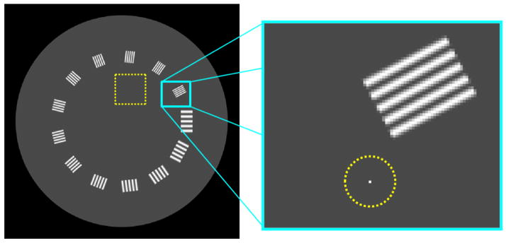
Digital phantom used for investigation of imaging performance of various reconstruction algorithms. The phantom is comprised of line pair blocks (from 7 lp/cm to 19 lp/cm), a uniform water-equivalent background with a square region-of-interest identified with dotted line used for empirical variance estimates, and a point target identified in a zoomed region that was used for estimating the reconstructed spatial resolution. The phantom is composed of 700x700 0.1 mm voxels.

Five different reconstruction approaches were investigated: 1) FBP – traditional filtered-backprojection of ordinary log-transformed data (i.e., no deblurring) using a raised cosine apodization; 2) UPWLS – quadratically penalized weighted least-squares estimation of ordinary log-transformed data with an uncorrelated noise model (K_l=D_q); 3) Deblur+FBP – deblurred projections using the transformation in (4) followed by filtered-backprojection with raised cosine apodization; 4) Deblur+UPWLS – deblurred projections followed by penalized weighted least-squares with an uncorrelated noise model (K_l=D_q); and 5) Deblur+CPWLS – deblurred projections followed by penalized weighted least-squares with the correlated noise model in (4). Each of these approaches allows for control of the noise-resolution trade-off in reconstruction: using a cut-off frequency in FBP methods, and adapting β in PWLS approaches. All PWLS techniques used 400 iterations of a conjugate gradients approach.

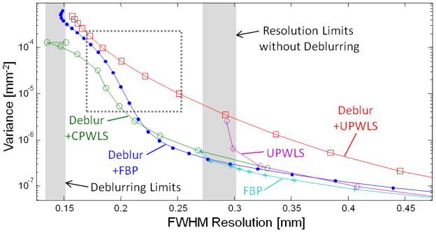
For each method a noise-resolution trade-off curve was generated in the following fashion. Reconstructions of both noisy and noiseless projection data over a range of parameter settings (cut-off frequency for FBP and β for PWLS) were performed. For each noisy reconstruction the variance in a uniform (artifact-free) region of the phantom (see Figure 1) was computed. For each noiseless reconstruction a point target in the reconstruction was fit to a Gaussian kernel to estimate the spatial resolution of the reconstruction. (Noiseless data was used to approximate the mean reconstruction and eliminate any fitting to noise.) Thus, these two values correspond to one point on a noise-resolution tradeoff curve with the entire parameter sweep identifying the achievable performance characteristics of each algorithm. These curves are plotted in Figure 2. It is important to note that not all spatial resolutions are achievable by a given algorithm. There resolution limits for each algorithm due to fundamental limits of sampling and geometry, as well as the reconstruction model. The resolution limits fall into two categories based on whether the reconstruction attempted to deblur projection data or did not include deblurring. Specifically, traditional approaches without deblurring were limited at ~0.275 mm FWHM resolution, whereas the deblurring approaches were able to achieve resolutions down to ~0.15 mm FWHM. As one would expect, across all methods, finer spatial resolutions are associated with higher noise in the reconstruction. At more coarse resolutions (above 0.3 mm FWHM), all of the methods except Deblur+UPWLS, performed comparably (note the logarithmic noise scale), suggesting that blur modeling is not particularly important if only moderate spatial resolutions are needed. The relatively poor performance of Deblur+UPWLS is somewhat unexpected. It appears that having the wrong noise model in this case for the deblurred data is worse than having no noise model at all (i.e., Deblur+FBP). In the high spatial resolution regime the proposed methods, Deblur+CPWLS, generally outperforms the other approaches. This is investigated in greater detail in Figure 3, which is a zoomed version of Figure 2.

Figure 2.

Resolution versus noise plots for various reconstruction methods. Traditional approaches that do not model detector blur cannot achieve spatial resolutions below approximately 0.275 mm FWHM resolution, whereas approaches that include deblurring can achieve resolutions down to about 0.15 mm with increased noise. These limits are marked with gray vertical bands. The proposed approach provides the best noise-resolution tradeoffs for the finest resolution reconstructions. A zoomed region of this plot (dotted rectangle) is discussed in Figure 3.

Figure 3.

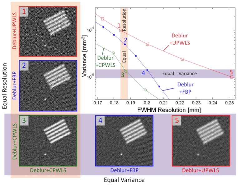
Relative performance of deblurring reconstruction approaches in the high spatial resolution regime. Both resolution-noise curves for each method and zoomed reconstructions that are either nearly matched in resolution (1–3) or nearly matched in noise (3–5) are presented. The points on the noise-resolution curve representing these reconstructions fall within the orange vertical band for the equal resolution cases, or within the purple horizontal band for equal variance cases. The improved noise handling of Deblur+CPWLS over other approaches at matched resolution is apparent in the background noise. Similarly, the improved spatial resolution of Deblur+CPWLS at matched noise is evident, particularly in resolving the line pairs. (Note some artifacts are apparent in the lower right, particularly in FBP, associated with line pairs on the opposite side of the phantom.)

Figure 3 concentrates on the performance of the three deblurring approaches at high spatial resolutions. In addition to showing the noise-resolution curves, (zoomed) reconstructions for these methods are also shown. Specifically, we have included reconstructions for each technique at nearly matched noise levels of ~1.1x10⁻⁵ mm⁻² (horizontal band), and at nearly matched spatial resolutions at ~0.186 mm FWHM (vertical band). For matched spatial resolutions, the order of magnitude decrease in variance between Deblur+UPWLS and Deblur+CPWLS, and the variance reduction factor of ~3.8 between Deblur+FBP and Deblur+CPWLS is readily apparent in the reconstruction. Similarly, at matched noise, the fine resolution of Deblur+CPWLS and the more coarse resolution of Deblur+FBP and Deblur+UPWLS are particularly conspicuous in the 19 lp/cm features.

CONCLUSION

In this paper a novel reconstruction approach that models both system blur and correlated noise was introduced and applied to simulated data. Not only does this approach allow for reconstruction of finer spatial resolution features than traditional methods that do not include blur models, but the proposed method also better handles the noise in the reconstructed images than approaches without a noise model or an incorrect noise model. Thus, the proposed methodology provides a tool for breaking traditional spatial resolution limits with better noise control. This methodology could have particular impact in high-resolution imaging scenarios like flat-panel CBCT for mammography, temporal bone imaging, quantitative analysis of trabecular bone analysis, etc. where traditional systems often have difficult resolving some of the fine structures pertinent to the diagnostic task.

References

- 1.Thibault JB, Sauer KD, Bouman CA, et al. A three-dimensional statistical approach to improved image quality for multislice helical CT. Med Phys. 2007;34(11):4526–44. doi: 10.1118/1.2789499. [DOI] [PubMed] [Google Scholar]
- 2.Yoon MA, Kim SH, Lee JM, et al. Adaptive statistical iterative reconstruction and Veo: assessment of image quality and diagnostic performance in CT colonography at various radiation doses. J Comput Assist Tomogr. 2012;36(5):596–601. doi: 10.1097/RCT.0b013e31826092be. [DOI] [PubMed] [Google Scholar]
- 3.De Man B, Basu S. Distance-driven projection and backprojection in three dimensions. Phys Med Biol. 2004;49(11):2463–75. doi: 10.1088/0031-9155/49/11/024. [DOI] [PubMed] [Google Scholar]
- 4.Long Y, Fessler JA, Balter JM. 3D forward and back-projection for X-ray CT using separable footprints. IEEE Trans Med Im. 2010;29(11):1839–50. doi: 10.1109/TMI.2010.2050898. [DOI] [PMC free article] [PubMed] [Google Scholar]
- 5.Yu DF, Fessler JA, Ficaro EP. Maximum-likelihood transmission image reconstruction for overlapping transmission beams. IEEE Trans Med Imaging. 2000;19(11):1094–105. doi: 10.1109/42.896785. [DOI] [PubMed] [Google Scholar]
- 6.Feng B, Fessler JA, King MA. Incorporation of system resolution compensation (RC) in the ordered-subset transmission (OSTR) algorithm for transmission imaging in SPECT. IEEE Trans Med Imaging. 2006;25(7):941–9. doi: 10.1109/tmi.2006.876151. [DOI] [PubMed] [Google Scholar]
- 7.Whiting B, Earl O, Snyder D, et al. X-ray CT signal statistics. Medical Physics. 2004;31(6):1744–1744. [Google Scholar]
- 8.Nuyts J, De Man B, Fessler JA, et al. Modelling the physics in the iterative reconstruction for transmission computed tomography. Phys Med Biol. 2013;58(12):R63–96. doi: 10.1088/0031-9155/58/12/R63. [DOI] [PMC free article] [PubMed] [Google Scholar]
- 9.Alessio A, Sauer K, Kinahan P. Statistical image reconstruction from correlated data with applications to PET. Phys Med Biol. 2007;52(20):6133–50. doi: 10.1088/0031-9155/52/20/004. [DOI] [PMC free article] [PubMed] [Google Scholar]
- 10.La Riviere PJ, Bian J, Vargas PA. Penalized-likelihood sinogram restoration for computed tomography. IEEE Trans Med Imaging. 2006;25(8):1022–36. doi: 10.1109/tmi.2006.875429. [DOI] [PubMed] [Google Scholar]