Más-o-menos: a simple sign averaging method for discrimination in genomic data analysis

Abstract

Motivation: The successful translation of genomic signatures into clinical settings relies on good discrimination between patient subgroups. Many sophisticated algorithms have been proposed in the statistics and machine learning literature, but in practice simpler algorithms are often used. However, few simple algorithms have been formally described or systematically investigated.

Results: We give a precise definition of a popular simple method we refer to as más-o-menos, which calculates prognostic scores for discrimination by summing standardized predictors, weighted by the signs of their marginal associations with the outcome. We study its behavior theoretically, in simulations and in an extensive analysis of 27 independent gene expression studies of bladder, breast and ovarian cancer, altogether totaling 3833 patients with survival outcomes. We find that despite its simplicity, más-o-menos can achieve good discrimination performance. It performs no worse, and sometimes better, than popular and much more CPU-intensive methods for discrimination, including lasso and ridge regression.

Availability and Implementation: Más-o-menos is implemented for survival analysis as an option in the survHD package, available from http://www.bitbucket.org/lwaldron/survhd and submitted to Bioconductor.

Contact: sdzhao@illinois.edu

1 INTRODUCTION

The successful translation of genomic signatures into clinical settings relies on good discrimination between patient subgroups that should receive different clinical management. Relatively, sophisticated methods such as penalized regression, support vector machines, random forests, bagging and boosting have seen detailed treatments in the statistics and machine learning literature (Bühlmann and Van De Geer, 2011; Hastie et al., 2005; Schölkopf and Smola, 2002); however, in practice many researchers prefer simpler algorithms (Hand, 2006). A systematic meta-analysis of prognostic models for late-stage ovarian cancer (Waldron et al., 2014) found that the most common methods in the field, and those used to generate the best-performing models on independent datasets, were of the ‘univariate ensemble’ type, where results of univariate regressions are aggregated to formulate a risk score.

The simplest of the univariate ensemble class of prediction methods sets the coefficients of a linear risk score for standardized covariates equal to the signs of their univariate associations with the clinical outcome of interest. In other words, for survival analysis it produces a risk score equal to the sum of the ‘bad prognosis’ features minus the sum of the ‘good prognosis’ features. This method and closely related variants can be found in the top clinical, bioinformatic and general science journals (Bell et al., 2011; Colman et al., 2010; Dave et al., 2004; Rème et al., 2013) and in commercially available prognostic gene signatures, such as the MyPRS signature for multiple myeloma prognosis (Shaughnessy et al., 2007). It has even been proposed, in a formula-free article, as a practical algorithm that can be performed in a spreadsheet with the ‘software and skill sets available to the cancer biologist’ (Hallett et al., 2010).

Despite the popularity and apparent effectiveness of this simplest of methods, to our knowledge, it has never been formally described or systematically investigated. We give a precise definition of the procedure and study its behavior theoretically, in simulations and in an extensive analysis of 27 independent gene expression studies of bladder, breast and ovarian cancer, altogether totaling 3833 patients with survival outcomes. We provide theoretical arguments that this method has good discrimination power and low variability when positively correlated features tend to have the same directions of marginal association with outcome. In simulations under a variety of sparsity and covariance structures, it performs competitively with lasso and ridge regression under all situations except the unlikely scenario of independent features, and was more than an order of magnitude faster. In application to survival analysis of three large microarray databases, it performed better than lasso and ridge regression in two of three cancer types, and comparably in the third. We refer to the method as más-o-menos because in Spanish the phrase ‘más o menos’ means both ‘plus or minus’, describing the method’s implementation, and ‘so-so’, describing its theoretically non-optimal but still practically useful discrimination ability.

2 METHODS

2.1 Más-o-menos

Let each component X_ij of the $p\times 1$ covariate vector $X_i={(X_{i1},\dots ,X_{ip})}^T$ be a quantitative measurement of the j^th gene from the i^th subject. The X_ij could represent various types of genomic information, such as expression levels from microarrays or next-generation sequencing experiments, or non-genomic data. Más-o-menos uses a patient’s $X_i$ to calculate a signed sum of that patient’s covariate values. The procedure is as follows:

1. Standardize the covariates such that ${(n-1)}^{-1}{\displaystyle \sum {(X_{ij}-{\overline{X}}_j)}^2}=1,j=1,\dots ,p$, where ${\overline{X}}_j=n^{-1}{\displaystyle \sum _i{X}_{ij}}$.

2. Perform univariate regressions of the outcome on each gene to obtain marginal estimates of the regression coefficient ${\widehat{\alpha }}_j$.

3. Let ${\widehat{v}}_j=\text{sgn}({\widehat{\alpha }}_j)/p^{1/2}$, where $\text{sgn}(c)=2I(c>0)-1$ for $c\ne 0$ and $\text{sgn}(c)=0$ for c = 0.

4. The risk score for the i^th patient is calculated as $X_i^T\widehat{v}$, where $\widehat{v}={({\widehat{v}}_1,\dots ,{\widehat{v}}_p)}^T$.

The factor of $p^{1/2}$ in the definition of the ${\widehat{v}}_j$ merely serves to ensure the arbitrary scaling $||\widehat{v}|{|}_2=1$. By changing the regression model used in step (3), más-o-menos can be used with clinical outcomes of any type, such as continuous, binary or censored data. The discrimination performance of $X_i^T\widehat{v}$ can be quantified using correlation for continuous outcomes, the area under the receiver operating characteristic curve for binary outcomes (Bamber, 1975) or the C-statistic for censored outcomes (Uno et al., 2011).

Más-o-menos, and procedures similar to it, is already in use for analyzing genomic data. For example, Donoho and Jin (2008) introduced a family of classifiers, one of which, called HCT-clip, is equivalent to más-o-menos. They found that HCT-clip performed surprisingly well in cross-validation experiments using standard datasets with uncensored outcomes. Some also use marginal regression to identify good and bad prognosis covariates, which are then used to rank patients by risk. Ranking methods include the t-statistic for difference in expression of good versus bad prognosis genes (Bell et al., 2011; Verhaak et al., 2013) and signed averaging of discretized or continuous expression values (Colman et al., 2010; Dave et al., 2004; Hallett et al., 2010; Kang et al., 2012; Rème et al., 2013). Replacing lasso coefficients by their signs has been proposed for summarizing gene pathway activity (Eng et al., 2013).

It may sometimes be helpful to perform an initial feature selection step before implementing más-o-menos, as we argue in Section 2.3. Feature selection has been the subject of a great deal of research, and a detailed discussion is beyond the scope of this article. In our data analysis in Section 3.3, we found that selection had little effect on the discrimination ability of más-o-menos. However, selection can provide more interpretable models by dramatically reducing the number of genes required for prediction.

2.2 Discrimination for survival outcomes

We focus on survival outcomes because they are typically the most difficult to deal with and the most clinically relevant and are the outcomes collected in our real data. Let T_i be the survival time of the i^th subject. To measure discrimination in the survival setting, we use the C-statistic over the follow-up period $(0,\tau )$, defined by Uno et al. (2011) as

$$C_{\tau }(\mathit{\beta })=P\{g(X_i)>g(X_j)|T_i<T_j,T_i<\tau \},$$ (1)

where $g(X)$ is the risk score for a subject with covariate vector X. We consider linear risk scores of the form $g(X)=X^T\mathit{\beta }$ for $\mathit{\beta }={({\beta }_1,\dots ,{\beta }_p)}^T$. We define the optimal weight vector to be

$${\mathit{\beta }}_0=\underset{{}_{\mathit{\beta }:{\left|{\mathit{\beta }}_0\right|}_2=1}}{\text{arg}\text{max}}P(X_i^T\mathit{\beta }>X_j^T\mathit{\beta }|T_i<T_j,T_i<\tau ),$$

where we have arbitrarily scaled ${\mathit{\beta }}_0$ to have norm 1 because $C_{\tau }(\mathit{\beta })$ is invariant to scaling of β.

To implement más-o-menos in this setting, we will obtain the ${\widehat{\alpha }}_j$ by fitting univariate Cox models. We choose the Cox model because it is a well-established and well-understood procedure in clinical research. In addition, the estimators ${\widehat{\alpha }}_j$ converge to well-defined ${\alpha }_{0j}$ even when the Cox model is not correctly specified (Lin and Wei, 1989; Struthers and Kalbfleisch, 1986), as is likely to be the case in our marginal regressions. Finally, if the data truly come from a Cox model, the true parameter vector should maximize $C_{\tau }$ and should be a scalar multiple of the optimal ${\mathit{\beta }}_0$.

2.3 Statistical properties

We show that under certain conditions, the más-o-menos weights can have good discrimination power along with low variability. Hand (2006) provided similar arguments to justify equalization of regression coefficients when all covariates have the same directions of effect on the outcome, and this direction is known a priori. Hand describes this in terms of the ‘flat maximum effect’: that in the context of classifiers, often little advantage can be gained in prediction accuracy over simple models. Here, we do not assume that the directions of effect are known.

Let $v^{*}={(v_1^{*},\dots ,v_p^{*})}^T$ be the probability limit of $\widehat{v}$, such that $\widehat{v}\to v^{*}$. Because ${\widehat{v}}_j=\text{sgn}({\widehat{\alpha }}_j)$, if ${\widehat{\alpha }}_j\to {\alpha }_{0j}$ in probability, then by the continuous mapping theorem $v_j^{*}=\text{sgn}({\alpha }_{0j})$. We will analyze the performance of the más-o-menos estimator $\widehat{v}$ in terms of the discrimination ability of $v^{*}$ relative to that of ${\mathit{\beta }}_0$, and the variability of $\widehat{v}$ around $v^{*}$. For now, we assume $v_j^{*}\ne 0$ for all genes j. At the end of the section we discuss the implications if this is not true.

By the definition of $C_{\tau }$, the discrimination performance of $v^{*}={(v_1^{*},\dots ,v_p^{*})}^T$ depends only on the degree of linear association between $X_i^T{\mathit{\beta }}_0$ and $X_i^T{v}^{*}$. In addition,

$$\begin{array}{l}\text{cov}(X_i^T{\mathit{\beta }}_0,X_i^T{v}^{*})={\displaystyle \sum _{j,k}{\beta }_{0j}}\text{cov}(X_{ij},X_{ik}{v}_k^{*})\\ ={\displaystyle \sum _j{\beta }_{0j}}{v}_j^{*}{\displaystyle \sum _k\text{cov}}(X_{ij}{v}_j^{*},X_{ik}{v}_k^{*})\ge \overline{\rho }{\displaystyle \sum _j{\beta }_{0j}}{v}_j^{*},\end{array}$$

where $\overline{\rho }={\min }_j{p}^{-1}\sum _k\text{cov}(X_{ij}{v}_j^{*},X_{ik}{v}_k^{*})$. The second equality follows because $v_j^{*}·v_j^{*}$ always equals 1. Thus, $X_i^T{v}^{*}$ will be highly correlated with $X_i^T{\mathit{\beta }}_0$, and will have similar discriminative ability, under the condition that ${\displaystyle \sum _j{\beta }_{0j}}{v}_j^{*}$ and $\overline{\rho }$ have the same sign.

It is not unreasonable to expect these terms to be positive. First, each ${\beta }_{0j}$ quantifies the association between X_ij and T_i conditional on all genes in $X_i$, while each $v_j^{*}$ reflects its univariate association. If a gene has the same direction of effect in both the conditional and marginal models, then ${\beta }_{0j}{v}_j^{*}>0$. This is plausible for at least some genes, and even if it does not hold for all genes $\sum _j{\beta }_{0j}{v}_j^{*}$ can still be positive. Second, the $\overline{\rho }$ term is the minimum average covariance between $X_{ij}{v}_j^{*}$ and $X_{ik}{v}_k^{*}$. This will be positive if genes with the same marginal directions of effect tend to be positively correlated, while genes with different marginal directions of effect tend to be negatively correlated. Indeed, the encoded proteins of conserved co-expressed gene pairs are likely to be part of the same biological pathway (van Noort et al., 2003). Again, $\overline{\rho }$ can be positive even if this covariance condition holds only for some pairs of genes, as we merely need the average covariance to be positive.

Restricting the más-o-menos weights to be either +1 or −1 endows it with low variability, which has been shown to be especially important in classification (Friedman, 1997). The variability of ${\widehat{v}}_j$ is given by

$$P({\widehat{v}}_j\ne v_j^{*})=\{\begin{array}{cc}P({\widehat{\alpha }}_j<0)& \text{if}{\alpha }_{0j}>0,\\ P({\widehat{\alpha }}_j>0)& \text{if}{\alpha }_{0j}<0,\\ P({\widehat{\alpha }}_j\ne 0)& \text{if}{\alpha }_{0j}=0.\end{array}$$

Lin and Wei (1989) showed that ${\widehat{\alpha }}_j\to N({\alpha }_{0j},{\sigma }_j^2/n)$ for some ${\alpha }_{0j}$ and ${\sigma }_j^2$. This approximation, combined with Mill’s inequality, gives the approximate relation

$$P({\widehat{v}}_j\ne v_j^{*})\mathrm{\lesssim }\frac{{\sigma }_j}{n^{1/2}|{\alpha }_{0j}|\sqrt{2\pi }}\exp \left(-\frac{1}{2}\frac{{\alpha }_{0j}^{2}n}{{\sigma }_j^2}\right)$$

when ${\alpha }_{0j}\ne 0$, which approaches 0 much faster than $\text{var}({\widehat{\alpha }}_j)$. For large n and/or large $|{\alpha }_{0j}|$, the variability of ${\widehat{v}}_j$ will be close to zero. Thus, $\widehat{v}$ is likely to be less susceptible to overfitting and, as a result, can have better out-of-sample discrimination performance.

Difficulties arise when $v_j^{*}=0$ for some marginally unimportant genes j. First, $\text{cov}(X_i^T{\mathit{\beta }}_0,X_i^T{v}^{*})$ will depend in part on the covariances between these genes and the marginally important ones, and it is unclear how these covariances will behave. Second, as ${\widehat{\alpha }}_j$ is a continuous estimator, $P({\widehat{\alpha }}_j\ne 0)$ will equal 1 for any sample size. In other words, más-o-menos may be less predictive and more variable when used on data where many of the covariates are not marginally associated with the outcome. An initial feature screening step may remove many such covariates, so that there are few j such that ${\alpha }_{0j}=0$. On the other hand, because gene expression levels tend to be correlated, even genes not involved in the disease process may be correlated to important genes and may have non-zero marginal associations.

3 RESULTS

3.1 Competing methods

We compared más-o-menos to three popular analysis methods that also generate linear risk scores, lasso (Tibshirani, 1996, 1997), ridge regression (Hoerl and Kennard, 1970; Verweij and Van Houwelingen, 1994) and marginal regression (Emura et al., 2012), which gives risk scores of the form $\sum _j{X}_{ij}{\widehat{\alpha }}_j$. For all methods we first standardized all covariates to have unit variance. We also included two negative controls: (i) the single gene with the largest ${\widehat{\alpha }}_j$ estimated from the training set and (ii) randomly generated risk scores $\sum _j{X}_{ij}{Z}_j$, where the Z_j were drawn independently from a standard normal.

We implemented lasso and ridge regression for the Cox model using the package glmnet (Friedman et al., 2010), selecting the penalty parameter using 3-fold cross-validation using the built-in function. Marginal Cox regressions and más-o-menos are implemented in the package survHD (Bernau et al., 2012).

3.2 Simulations

To simulate training data, we generated $p\times 1$ covariate vectors $X_i$ and survival times from a Cox model with a $p\times 1$ true parameter vector ${\mathit{\beta }}_0$. We let the true Cox regression coefficient vector ${\mathit{\beta }}_0$ have s non-zero components all with magnitude $s^{-1/2}$, such that ${||{\mathit{\beta }}_0||}_2=1$. The first $s/2$ non-zero components were positive and the rest were negative. We generated censoring times from an independent exponential distribution to give ∼50% censoring. In each testing dataset, we replaced the positive entries of ${\mathit{\beta }}_0$ by random uniform draws from $(0,4/s^{1/2})$, and the negative entries by random draws from $(-4/s^{1/2},0)$. Each training and testing dataset contained n = 200 observations.

We considered the low-dimensional case of P = 100 and the high-dimensional one of P = 10 000. To generate sparse ${\mathit{\beta }}_0$, we let s = 10, and for non-sparse ${\mathit{\beta }}_0$ we let s = P. We drew $X_i$ from a multivariate normal with mean zero and unit marginal variance. From Section 2.3, the discrimination ability of más-o-menos depends on the covariance structure of the $X_i$. In an ‘easy’ setting, the covariates were divided into two blocks, with X_ij positively correlated within blocks and negatively correlated between blocks. Those X_ij with ${\beta }_{0j}>0$ were assigned to one block, those with ${\beta }_{0j}<0$ were assigned to the other and those with ${\beta }_{0j}=0$ were assigned equally between the blocks. In a ‘hard’ setting, we let $\text{cov}(X_{ij},X_{ik})>0$ for j and k both even or both odd, and $\text{cov}(X_{ij},X_{ik})<0$ otherwise. We let $|\text{cov}(X_{ij},X_{ik})|=0$, 0.3 or 0.5 for all j and k and ran 200 simulations.

The computations in this article were run on the Odyssey cluster supported by the Faculty of Arts and Sciences (FAS) Science Division Research Computing Group at Harvard University. Table 1 illustrates the speed advantage enjoyed by más-o-menos.

Table 1.

Average simulation runtimes

Method	P = 100	P = 10 000
Lasso	8.914	47.238
Ridge	0.645	30.124
Marginal	0.016	2.209
Más-o-menos	0.023	2.408
Single	0.017	1.674
Random	0.001	0.004

Runtimes are reported in seconds

In general, más-o-menos kept pace with lasso, ridge and marginal regression. Each of these performed better than the single best gene and the randomly generated negative control. Figure 1 reports the average out-of-sample C-statistics obtained by the different methods. The C-statistics were calculated at $\tau =2$, where τ is defined in (1). Confidence intervals represent the empirical 2.5 and 97.5% quantiles. The results clearly illustrate the importance of the covariance structure. All of the methods except for the negative control performed better under the easy covariance setting than under the hard one. The easy covariance satisfies the assumptions of the theoretical discussion in Section 2.3: $\text{cov}(X_{ij}{v}_j^{*},T_i)>0$ and $\text{cov}(X_{ij}{v}_j^{*},X_{ik}{v}_k^{*})>0$ for all j, k. The difficulty of the hard covariance structure arises from the fact that it is impossible to meet this condition. For example, by construction, $\text{cov}(X_{i1},T_i)>0$ and $\text{cov}(X_{i2},T_i)>0$, but $\text{cov}(X_{i1},X_{i2})<0$. In other words, the signs of the ${\beta }_{0j}$ and the covariances are incoherent in the hard covariance case.

Fig. 1.

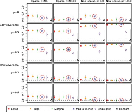
Average validation C-statistics of different discrimination methods in simulated data. Más-o-menos results highlighted by circle. Vertical bars represent confidence intervals

When the covariates were independent, higher dimensionality made discrimination harder regardless of sparsity, perhaps because there was no way to borrow information across the covariates. Under the easy covariance structure with a dense ${\mathit{\beta }}_0$, however, high dimensionality was actually beneficial, perhaps because if the effects of some covariates were by chance incorrectly estimated, there were many other correlated ones that could be used as surrogates. On the other hand, with a hard covariance matrix, dimensionality added difficulty even in the non-sparse case because of the incoherence between the ${\beta }_{0j}$ and the covariate correlations.

With no correlation, sparsity allowed for easier discrimination. When correlation was introduced in the easy covariance setting, sparsity was detrimental to prediction. This might have been owing to the screening step because univariate screening is liable to retain unimportant covariates simply because they are correlated with important ones. These incorrectly retained covariates can degrade performance. In the hard covariance setting, however, sparsity was helpful regardless of the level of correlation. This may be because in the sparse case, there were fewer important covariates with which the hard covariance structure could cause difficultly.

3.3 Application to bladder, breast and ovarian cancer

We applied más-o-menos, lasso, ridge, marginal regression and the two negative control methods to an extensive compendium of real cancer gene expression data (Table 2). We obtained six bladder cancer datasets totaling 679 patients from Riester et al. (2012), seven breast cancer datasets totaling 1709 patients from Haibe-Kains et al. (2012) and 14 ovarian cancer datasets totaling 1445 patients from Ganzfried et al. (2013). We processed the breast cancer data as in Bernau et al. (2014). The bladder and ovarian cancer data have been manually curated to have standardized clinical annotations, probeset identifiers and microarray preprocessing, and are available in the Bioconductor packages curatedBladderData and curatedOvarianData, respectively.

Table 2.

Cancer gene expression datasets

Reference	Sample size	Events
Bladder, 2463 common probesets
Als et al. (2007)	30	25
Blaveri et al. (2005)	80	44
Kim et al. (2010)	165	69
Lindgren et al. (2010)	87	26
Riester et al. (2012)	93	65
Sjödahl et al. (2012)	224	25
Breast, 9768 common probesets
Desmedt et al. (2007)	134	35
Foekens et al. (2006)	710	191
Minn et al. (2005)	245	76
Minn et al. (2007); Wang et al. (2005)	209	80
Schmidt et al. (2008)	162	33
Sotiriou et al. (2006)	85	19
Symmans et al. (2010)	164	38
Ovarian, 6138 common probesets
Bentink et al. (2012)	128	73
Crijns et al. (2009)	98	72
Bonome et al. (2008)	185	129
Denkert et al. (2009)	41	13
Dressman et al. (2007)	59	36
Ferriss et al. (2012)	30	22
Konstantinopoulos et al. (2010)	28	17
Konstantinopoulos et al. (2010)	42	23
Mok et al. (2009)	53	41
Bell et al. (2011)	452	239
Tothill et al. (2008)	140	72
Yoshihara et al. (2010)	43	22
Yoshihara et al. (2012)	129	60
Yoshihara et al. (2012)	17	10

For each disease, we limited our analyses to the probesets common to all studies. We trained each algorithm on the largest available study and evaluated its performance on each of the remaining datasets using the C-statistic calculated at $\tau =5$ years, where τ is defined in (1). Roughly 60% of all study participants, combined across all diseases, were still alive after 5 years. The C-statistic is robust to the choice of τ unless few deaths or censoring events occur at times greater than τ (Uno et al., 2011).

We generated 100 bootstrap samples of each validation dataset to obtain 95% confidence intervals. In addition to applying the methods without feature selection, we also implemented higher criticism thresholding (Donoho and Jin, 2008), which screens out covariates with high marginal Cox regression P-values but is entirely data-driven and automatically chooses the number of covariates to retain. Summary statistics were calculated by fixed effects meta-analysis with the metafor package (Viechtbauer, 2010).

Figure 2 reports the results. Selecting only a single gene or using random weights gave the lowest performance, confirming the appropriateness of our negative controls. Más-o-menos was consistently on par with lasso, and even outperformed lasso in several cases. Its performance was much more similar to those of ridge and marginal regression. Screening did not dramatically affect the performances of any of the methods.

Fig. 2.

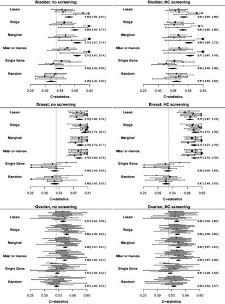
Validation C-statistics at $\tau =5$ years using different discrimination methods

A referee noted that it is unclear how well más-o-menos performs within a single dataset, as opposed to across datasets. To answer this question, we evaluated the performance of each risk prediction algorithm within each dataset of each disease type by calculating the average 3-fold cross-validated C-statistic at $\tau =5$ years. No feature screening was implemented. Figure 3 reports the results and shows that más-o-menos was again on par or better than the other methods. It appears that in addition to being robust across studies, más-o-menos is also simply a good predictor.

Fig. 3.

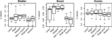
Average 3-fold cross-validation C-statistics at $\tau =5$ years, calculated within each dataset of each disease type; no feature screening was implemented

4 DISCUSSION

We have studied más-o-menos, a simple algorithm for classification and discrimination that has seen popular adoption but has not been formally investigated. We gave a precise definition of the algorithm, showed theoretically and in simulations that it can perform well and demonstrated in an extensive analysis of real cancer gene expression studies that it can achieve good discrimination performance in realistic settings, even compared with lasso and ridge regression. Our results provide some justification to support its widespread use in practice. We hope our work will help shift the emphasis of ongoing prediction modeling efforts in genomics from the development of complex models to the more important issues of study design, model interpretation and independent validation.

One reason why más-o-menos is comparable with more sophisticated methods such as penalized regression may be that we often use a prediction model trained on one set of patients to discriminate between subgroups in an independent sample, usually collected from a slightly different population and processed in a different laboratory. This cross-study variation is not captured by standard theoretical analyses, so theoretically optimal methods may not perform well in real applications (Hand, 2006). Bernau et al. (2014) proposed a method for giving a realistic measure of the practical utility of algorithms in the presence of cross-study variation. At the same time, we found using cross-validation experiments that even within the same dataset, más-o-menos remained competitive with more sophisticated methods.

Batch effects create study-specific measurement bias, and are widespread and often unidentified in genomic data (Leek et al., 2010). They may be responsible for the cross-study variation that degrades the performance of algorithms such as lasso or ridge regression. Although certain batch-correction techniques have gained widespread use (Leek and Storey, 2007; Li and Rabinovic, 2007), these have been motivated primarily by class comparison rather than class prediction. In a genomic prediction competition, batch correction was seen to provide no overall benefit for validation accuracy (MAQC Consortium, 2010). Rather, we propose that the impact of unknown batch effects may be best mitigated by using methods less prone to over-fitting. Más-o-menos risk scores have lower variability, and may be less associated with batch, than those of the other methods, which might explain its robust performance in both cross-validation and cross-study validation in 27 datasets from three cancer types.

While we focused on microarray data and survival endpoints, más-o-menos can be applied to any type of outcome variable, using any regression model, and has precedents for application in diverse settings outside of genomics (Davis-Stober et al., 2010; Wainer, 1976; Laughlin, 1978; Lovie and Lovie, 1986). It is fast to implement, simple to interpret, comparable in performance with more complex methods and appears robust to cross-study variation. Más-o-menos should be useful for developing prediction models from high-dimensional data in any situation where the covariates are sufficiently correlated and the true effect is roughly linear.

REFERENCES

- Als AB, et al. Emmprin and survivin predict response and survival following cisplatin-containing chemotherapy in patients with advanced bladder cancer. Clin. Cancer Res. 2007;13:4407–4414. doi: 10.1158/1078-0432.CCR-07-0109. [DOI] [PubMed] [Google Scholar]
- Bamber D. The area above the ordinal dominance graph and the area below the receiver operating characteristic graph. J. Math. Psychol. 1975;12:387–415. [Google Scholar]
- Bell D, et al. Integrated genomic analyses of ovarian carcinoma. Nature. 2011;474:609–615. doi: 10.1038/nature10166. [DOI] [PMC free article] [PubMed] [Google Scholar]
- Bentink S, et al. Angiogenic mRNA and microRNA gene expression signature predicts a novel subtype of serous ovarian cancer. PloS One. 2012;7:e30269. doi: 10.1371/journal.pone.0030269. [DOI] [PMC free article] [PubMed] [Google Scholar]
- Bernau C, et al. survHD: Synthesis of Microarray-based Survival Analysis. 2012. R package version 0.5.0. https://bitbucket.org/lwaldron/survhd. [Google Scholar]
- Bernau C, et al. Cross-study validation for assessment of prediction models and algorithms. Bioinformatics. 2014;30:i105–i112. doi: 10.1093/bioinformatics/btu279. [DOI] [PMC free article] [PubMed] [Google Scholar]
- Blaveri E, et al. Bladder cancer outcome and subtype classification by gene expression. Clin. Cancer Res. 2005;11:4044–4055. doi: 10.1158/1078-0432.CCR-04-2409. [DOI] [PubMed] [Google Scholar]
- Bonome T, et al. A gene signature predicting for survival in suboptimally debulked patients with ovarian cancer. Cancer Res. 2008;68:5478–5486. doi: 10.1158/0008-5472.CAN-07-6595. [DOI] [PMC free article] [PubMed] [Google Scholar]
- Bühlmann P, Van De Geer S. Statistics for High-dimensional Data: Methods, Theory and Applications. Heidelberg: Springer; 2011. [Google Scholar]
- Colman H, et al. A multigene predictor of outcome in glioblastoma. Neuro-oncology. 2010;12:49–57. doi: 10.1093/neuonc/nop007. [DOI] [PMC free article] [PubMed] [Google Scholar]
- Crijns A, et al. Survival-related profile, pathways, and transcription factors in ovarian cancer. PLoS Med. 2009;6:e1000024. doi: 10.1371/journal.pmed.1000024. [DOI] [PMC free article] [PubMed] [Google Scholar]
- Dave SS, et al. Prediction of survival in follicular lymphoma based on molecular features of tumor-infiltrating immune cells. N. Engl. J. Med. 2004;351:2159–2169. doi: 10.1056/NEJMoa041869. [DOI] [PubMed] [Google Scholar]
- Davis-Stober C, et al. A constrained linear estimator for multiple regression. Psychometrika. 2010;75:521–541. [Google Scholar]
- Denkert C, et al. A prognostic gene expression index in ovarian cancer-validation across different independent data sets. J. Pathol. 2009;218:273–280. doi: 10.1002/path.2547. [DOI] [PubMed] [Google Scholar]
- Desmedt C, et al. Strong time dependence of the 76-gene prognostic signature for node-negative breast cancer patients in the transbig multicenter independent validation series. Clin. Cancer Res. 2007;13:3207–3214. doi: 10.1158/1078-0432.CCR-06-2765. [DOI] [PubMed] [Google Scholar]
- Donoho D, Jin J. Higher criticism thresholding: Optimal feature selection when useful features are rare and weak. Proc. Nat Acad. Sci. USA. 2008;105:14790–14795. doi: 10.1073/pnas.0807471105. [DOI] [PMC free article] [PubMed] [Google Scholar]
- Dressman H, et al. An integrated genomic-based approach to individualized treatment of patients with advanced-stage ovarian cancer. J. Clin. Oncol. 2007;25:517–525. doi: 10.1200/JCO.2006.06.3743. [DOI] [PubMed] [Google Scholar]
- Emura T, et al. Survival prediction based on compound covariate under cox proportional hazard models. PLoS One. 2012;7:e47627. doi: 10.1371/journal.pone.0047627. [DOI] [PMC free article] [PubMed] [Google Scholar]
- Eng KH, et al. Pathway index models for construction of patient-specific risk profiles. Stat. Med. 2013;32:1524–1535. doi: 10.1002/sim.5641. [DOI] [PMC free article] [PubMed] [Google Scholar]
- Ferriss JS, et al. Multi-gene expression predictors of single drug responses to adjuvant chemotherapy in ovarian carcinoma: predicting platinum resistance. PloS One. 2012;7:e30550. doi: 10.1371/journal.pone.0030550. [DOI] [PMC free article] [PubMed] [Google Scholar]
- Foekens JA, et al. Multicenter validation of a gene expression–based prognostic signature in lymph node–negative primary breast cancer. J. Clin. Oncol. 2006;24:1665–1671. doi: 10.1200/JCO.2005.03.9115. [DOI] [PubMed] [Google Scholar]
- Friedman JH. On bias, variance, 0/1loss, and the curse-of-dimensionality. Data Min. Knowl. Discov. 1997;1:55–77. [Google Scholar]
- Friedman JH, et al. Regularization paths for generalized linear models via coordinate descent. J. Stat. Softw. 2010;33:1–22. [PMC free article] [PubMed] [Google Scholar]
- Ganzfried BF, et al. curatedOvarianData: clinically annotated data for the ovarian cancer transcriptome. Database. 2013;2013:bat013. doi: 10.1093/database/bat013. [DOI] [PMC free article] [PubMed] [Google Scholar]
- Haibe-Kains B, et al. A three-gene model to robustly identify breast cancer molecular subtypes. J. Nat Cancer Inst. 2012;104:311–325. doi: 10.1093/jnci/djr545. [DOI] [PMC free article] [PubMed] [Google Scholar]
- Hallett RM, et al. An algorithm to discover gene signatures with predictive potential. J. Exp. Clin. Cancer Res. 2010;29:120. doi: 10.1186/1756-9966-29-120. [DOI] [PMC free article] [PubMed] [Google Scholar]
- Hand DJ. Classifier technology and the illusion of progress. Stat. Sci. 2006;21:1–14. [Google Scholar]
- Hastie T, et al. The elements of statistical learning: data mining, inference and prediction. Math. Intell. 2005;27:83–85. [Google Scholar]
- Hoerl A, Kennard R. Ridge regression: biased estimation for nonorthogonal problems. Technometrics. 1970;12:55–67. [Google Scholar]
- Kang J, et al. A dna repair pathway-focused score for prediction of outcomes in ovarian cancer treated with platinum-based chemotherapy. J. Nat Cancer Inst. 2012;104:670–681. doi: 10.1093/jnci/djs177. [DOI] [PMC free article] [PubMed] [Google Scholar]
- Kim WJ, et al. Predictive value of progression-related gene classifier in primary non-muscle invasive bladder cancer. Mol. Cancer. 2010;9:3. doi: 10.1186/1476-4598-9-3. [DOI] [PMC free article] [PubMed] [Google Scholar]
- Konstantinopoulos P, et al. Gene expression profile of BRCAness that correlates with responsiveness to chemotherapy and with outcome in patients with epithelial ovarian cancer. J. Clin. Oncol. 2010;28:3555–3561. doi: 10.1200/JCO.2009.27.5719. [DOI] [PMC free article] [PubMed] [Google Scholar]
- Laughlin JE. Comment on Estimating coefficients in linear models: it don’t make no nevermind. Psychol. Bull. 1978;85:247–253. [Google Scholar]
- Leek JT, Storey JD. Capturing heterogeneity in gene expression studies by surrogate variable analysis. PLoS Genet. 2007;3:e161–e161. doi: 10.1371/journal.pgen.0030161. [DOI] [PMC free article] [PubMed] [Google Scholar]
- Leek JT, et al. Tackling the widespread and critical impact of batch effects in high-throughput data. Nat. Rev. Genet. 2010;11:733–739. doi: 10.1038/nrg2825. [DOI] [PMC free article] [PubMed] [Google Scholar]
- Li C, Rabinovic A. Adjusting batch effects in microarray expression data using empirical Bayes methods. Biostatistics. 2007;8:118–127. doi: 10.1093/biostatistics/kxj037. [DOI] [PubMed] [Google Scholar]
- Lin D, Wei L. The robust inference for the Cox proportional hazards model. J. Am. Stat. Assoc. 1989;84:1074–1078. [Google Scholar]
- Lindgren D, et al. Combined gene expression and genomic profiling define two intrinsic molecular subtypes of urothelial carcinoma and gene signatures for molecular grading and outcome. Cancer Res. 2010;70:3463–3472. doi: 10.1158/0008-5472.CAN-09-4213. [DOI] [PubMed] [Google Scholar]
- Lovie A, Lovie P. The flat maximum effect and linear scoring models for prediction. J. Forecast. 1986;5:159–168. [Google Scholar]
- MAQC Consortium. The microarray quality control (maqc)-ii study of common practices for the development and validation of microarray-based predictive models. Nat. Biotechnol. 2010;28:827–865. doi: 10.1038/nbt.1665. [DOI] [PMC free article] [PubMed] [Google Scholar]
- Minn AJ, et al. Genes that mediate breast cancer metastasis to lung. Nature. 2005;436:518–524. doi: 10.1038/nature03799. [DOI] [PMC free article] [PubMed] [Google Scholar]
- Minn AJ, et al. Lung metastasis genes couple breast tumor size and metastatic spread. Proc. Nat Acad. Sci. USA. 2007;104:6740–6745. doi: 10.1073/pnas.0701138104. [DOI] [PMC free article] [PubMed] [Google Scholar]
- Mok S, et al. A gene signature predictive for outcome in advanced ovarian cancer identifies a survival factor: microfibril-associated glycoprotein 2. Cancer Cell. 2009;16:521–532. doi: 10.1016/j.ccr.2009.10.018. [DOI] [PMC free article] [PubMed] [Google Scholar]
- Rème T, et al. Modeling risk stratification in human cancer. Bioinformatics. 2013;29:1149–1157. doi: 10.1093/bioinformatics/btt124. [DOI] [PubMed] [Google Scholar]
- Riester M, et al. Combination of a novel gene expression signature with a clinical nomogram improves the prediction of survival in high-risk bladder cancer. Clin. Cancer Res. 2012;18:1323–1333. doi: 10.1158/1078-0432.CCR-11-2271. [DOI] [PMC free article] [PubMed] [Google Scholar]
- Schmidt M, et al. The humoral immune system has a key prognostic impact in node-negative breast cancer. Cancer Res. 2008;68:5405–5413. doi: 10.1158/0008-5472.CAN-07-5206. [DOI] [PubMed] [Google Scholar]
- Schölkopf B, Smola AJ. Learning with Kernels: Support Vector Machines, Regularization, Optimization, and Beyond. MIT press; 2002. [Google Scholar]
- Shaughnessy J, et al. A validated gene expression model of high-risk multiple myeloma is defined by deregulated expression of genes mapping to chromosome 1. Blood. 2007;109:2276–2284. doi: 10.1182/blood-2006-07-038430. [DOI] [PubMed] [Google Scholar]
- Sjödahl G, et al. A molecular taxonomy for urothelial carcinoma. Clin. Cancer Res. 2012;18:3377–3386. doi: 10.1158/1078-0432.CCR-12-0077-T. [DOI] [PubMed] [Google Scholar]
- Sotiriou C, et al. Gene expression profiling in breast cancer: understanding the molecular basis of histologic grade to improve prognosis. J. Nat Cancer Inst. 2006;98:262–272. doi: 10.1093/jnci/djj052. [DOI] [PubMed] [Google Scholar]
- Struthers C, Kalbfleisch J. Misspecified proportional hazard models. Biometrika. 1986;73:363–369. [Google Scholar]
- Symmans WF, et al. Genomic index of sensitivity to endocrine therapy for breast cancer. J. Clin. Oncol. 2010;28:4111–4119. doi: 10.1200/JCO.2010.28.4273. [DOI] [PMC free article] [PubMed] [Google Scholar]
- Tibshirani RJ. Regression shrinkage and selection via the lasso. J. R. Stat. Soc. Ser. B. 1996;58:267–288. [Google Scholar]
- Tibshirani RJ. The lasso method for variable selection in the Cox model. Stat. Med. 1997;16:385–395. doi: 10.1002/(sici)1097-0258(19970228)16:4<385::aid-sim380>3.0.co;2-3. [DOI] [PubMed] [Google Scholar]
- Tothill R, et al. Novel molecular subtypes of serous and endometrioid ovarian cancer linked to clinical outcome. Clin. Cancer Res. 2008;14:5198–5208. doi: 10.1158/1078-0432.CCR-08-0196. [DOI] [PubMed] [Google Scholar]
- Uno H, et al. On the c-statistics for evaluating overall adequacy of risk prediction procedures with censored survival data. Stat. Med. 2011;30:1105–1117. doi: 10.1002/sim.4154. [DOI] [PMC free article] [PubMed] [Google Scholar]
- van Noort V, et al. Predicting gene function by conserved co-expression. Trends Genet. 2003;19:238–242. doi: 10.1016/S0168-9525(03)00056-8. [DOI] [PubMed] [Google Scholar]
- Verhaak RG, et al. Prognostically relevant gene signatures of high-grade serous ovarian carcinoma. J. Clin. Invest. 2013;123:517. doi: 10.1172/JCI65833. [DOI] [PMC free article] [PubMed] [Google Scholar]
- Verweij P, Van Houwelingen H. Penalized likelihood in cox regression. Stat. Med. 1994;13:2427–2436. doi: 10.1002/sim.4780132307. [DOI] [PubMed] [Google Scholar]
- Viechtbauer W. Conducting meta-analyses in R with the metafor package. J. Stat. Softw. 2010;36:1–48. [Google Scholar]
- Wainer H. Estimating coefficients in linear models: it don’t make no nevermind. Psychol. Bull. 1976;83:213–217. [Google Scholar]
- Waldron L, et al. Comparative meta-analysis of prognostic gene signatures for Late-Stage ovarian cancer. J. Nat Cancer Inst. 2014;106 doi: 10.1093/jnci/dju049. pii: dju049. [DOI] [PMC free article] [PubMed] [Google Scholar]
- Wang Y, et al. Gene-expression profiles to predict distant metastasis of lymph-node-negative primary breast cancer. Lancet. 2005;365:671–679. doi: 10.1016/S0140-6736(05)17947-1. [DOI] [PubMed] [Google Scholar]
- Yoshihara K, et al. Gene expression profile for predicting survival in advanced-stage serous ovarian cancer across two independent datasets. PloS One. 2010;5:e9615. doi: 10.1371/journal.pone.0009615. [DOI] [PMC free article] [PubMed] [Google Scholar]
- Yoshihara K, et al. High-risk ovarian cancer based on 126-gene expression signature Is uniquely characterized by downregulation of antigen presentation pathway. Clin. Cancer Res. 2012;18:1374–1385. doi: 10.1158/1078-0432.CCR-11-2725. [DOI] [PubMed] [Google Scholar]