Massive parallelization of serial inference algorithms for a complex generalized linear model

Abstract

Following a series of high-profile drug safety disasters in recent years, many countries are redoubling their efforts to ensure the safety of licensed medical products. Large-scale observational databases such as claims databases or electronic health record systems are attracting particular attention in this regard, but present significant methodological and computational concerns. In this paper we show how high-performance statistical computation, including graphics processing units, relatively inexpensive highly parallel computing devices, can enable complex methods in large databases. We focus on optimization and massive parallelization of cyclic coordinate descent approaches to fit a conditioned generalized linear model involving tens of millions of observations and thousands of predictors in a Bayesian context. We find orders-of-magnitude improvement in overall run-time. Coordinate descent approaches are ubiquitous in high-dimensional statistics and the algorithms we propose open up exciting new methodological possibilities with the potential to significantly improve drug safety.

1 Motivation and Background

Increasing scientific, regulatory and public scrutiny focuses on the obligation of the medical community, pharmaceutical industry and health authorities to ensure that marketed drugs have acceptable benefit-risk profiles (Coplan et al., 2011). Longitudinal observational databases provide time-stamped patient-level medical information, such as periods of drug exposure and dates of diagnoses, and are emerging as important data sources for associating the occurrence of adverse events (AEs) with specific drug use in the post-marketing setting once drugs are in wide-spread clinical use (Stang et al., 2010). Some relevant papers focusing on drug safety from observation databases include Curtis et al. (2008); Jin et al. (2008); Li (2009); Norén et al. (2008); Schneeweiss et al. (2009); Kulldor et al. (2011) Typical examples of these observation databases encompass administrative medical claims databases and electronic health record systems, with larger claims databases containing upwards of 50 million lives with up to 10 years of data per life and exposure to 1000s of different drugs (Ryan et al., 2012).

The scale of these massive databases presents compelling computational challenges when attempting to estimate the strength of association between each drug and each of several AEs, while appropriately accounting for covariates such as other concomitant drugs, patient demographics and concurrent disease. Generalized linear models (GLMs) with unknown parameter regularization or Bayesian priors offer one thriving opportunity to estimate association strength while controlling for many other covariates (Madigan et al., 2011). However, naive implementation even to find maximum a posteriori (MAP) point-estimates in standard statistical packages grind to an almost stand-still with millions of outcomes and thousands of predictors, and hope of estimating even poor measures of uncertainty on drug-specific association estimates vanishes.

One usual approach to the computationally intensive task of statistical model fitting entertains distributing the work across a specialized and costly cluster or cloud of computers. This approach achieves most success when the distributed jobs consist of lengthy “embarrassingly parallel” (EP) operations, such as the independent simulation of whole Markov chains in MCMC (Wilkinson, 2006). However, the cluster with its distributed memory commands high communication latency between operations, rendering even MAP estimation in a GLM often unworkable, let alone estimation of second order terms such as standard errors. MAP estimation is generally an iterative algorithm, and the potentially parallizable work within each step is rarely sufficient to outweigh the communication latency and thread management costs.

For massive parallelization that overcomes many of these issues, there exists a much less expensive resource available in many desktop and laptop computers, the graphics processing unit (GPU); see, for example, Suchard et al. (2010) for a gentle introduction in statistical model fitting. GPUs are dedicated numerical processors originally designed for rendering 3-dimensional computer graphics. A GPU consists of tens to hundreds of processor cores on a single chip. These can be programmed to perform a sequence of numerical operations simultaneously to each element of a large data array. The acronym SPMD summarizes this single program, multiple data paradigm. Because the same operations, called kernels, function simultaneously, GPUs can achieve extremely high arithmetic intensity provided one can transfer input data and output results onto and off of the processors efficiently. Because the parallel threads driving the kernels operate on the same computer card, the cost of spawning and destroying millions of threads within each iterative step of the MAP estimation is neglible, and communication latency between threads is minimal. However, statisticians have been slow to embrace the new technology, due in part to a preconception that GPUs work best with EP operations. To dispell these ideas, Silberstein et al. (2008) first demonstrated the potential for GPUs in fitting simple Bayesian networks. Recently, Suchard and Rambaut (2009) and Suchard et al. (2010) have seen greater than 100-fold speed-ups in MCMC simulations involving highly structured graphical models and mixture models. Lee et al. (2010) and Tibbits et al. (2011) are following suit with Bayesian model fitting via particle filtering and slice sampling, and Zhou et al. (2010) demonstrate GPU utility for high-dimensional optimization.

In this paper, we explore the use of GPU parallelization in fitting a real-world problem involving a penalized GLM to massive observation datasets with high-throughput computing needs. We entertain recent advances in a Bayesian self-controlled case series (BSCCS) model (Madigan et al., 2011) and by exploiting the sparsity of the resulting database design matrix, we optimize a cyclic coordinate descent (CCD) algorithm to generate MAP estimates for this high-dimensional GLM. Given the substantial speed-up that optimization and the GPU afford, we provide for the first time rough estimates of the prior hyperparameters and limited measures of coefficient uncertainty.

2 Methods

GLMs assume subject outcomes arise from an exponential family distribution whose mean is a deterministic function of an outcome-specific linear predictor (Nelder and Wedderburn, 1972). These models include, for example, logistic regression, Poisson regression and several survival models. Often, study designs necessiate matching subjects or conditioning on sufficient statistics of the generative distribution to infer the relative effects of predictors; this leads to complex GLMs with likelihood-functions that grow computationally expensive in massive datasets. We explore one such model as a case-study in optimization and parallelization.

2.1 Bayesian Self-Controlled Case Series Model

Farrington (1995) proposed the self-controlled case series (SCCS) method in order to estimate the relative incidence of AEs to assess vaccine safety. SCCS provides a cases-only (subjects with at least one AE) design that automatically controls for time-fixed covariates. Since each subject serves as her own control, all individual-specific effects drop out of the model likelihood and the method compares AE rates between exposed and unexposed time-intervals through an underlying inhomogeneous Poisson process assumption.

Suppose an observational database tracks the drug exposure and AE history of i = 1, … , N subjects who each experience at least one AE. Figure 1 cartoons such a history. During observation, subjects start and stop individual regiments of j = 1, … , J possible drugs accumulated across all subjects. These regiments partition each subject’s observational period into k = 1, … , K_i eras, during which drug exposure is (assumed to be) constant. Drug exposure indicators x_ik = (x_ik1, … , x_ikJ)’ and time-lengths l_ik (generally recorded in days) fully characterize each era for each subject, where x_ikj = 1 if exposed to drug j or otherwise 0. Finally, y_ik counts the number of AEs for subject i during era k and, for convenience, we group y_i = (y_i1, … , y_iKi)’, x_i = (x_i1, … , x_iKi)’ and l_i = (l_i1, … , l_iKi)’.

Figure 1.

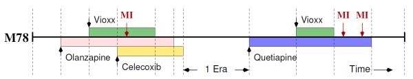
Representative drug exposure and adverse event (myocardial infarction, MI) history for one 78 year-old male. In constant exposure era k = 4, this subject suffers an MI (y_i,4 = 1) and is taking Vioxx, Olanzapine and Celecoxib (x_i,4,V = x_i,4,C = 1). In era k = 10, this subject suffers two MIs (y_i,10 = 2) and is taking Quetiapine (x_i,10,Q = 1).

A SCCS assumes that these AEs arise according to an inhomogeneous Poisson process, where a subject baseline effect e^ϕi and drug exposures multiplicatively modulate the underlying instantaneous event intensity ${\lambda }_{\mathit{ik}}=e^{{\varphi }_i+{\mathbf{x}}_{\mathit{ik}}^{\prime }\beta }$ for subject i during era k. Here, β = (β₁, … , β_J)’ are unknown relative risks attributable to each drug. Consequentially, y_ik ~ Poisson(λ_ik). Due to computational demand, researchers have typically applied this model to study only one potential exposure at a time, ignoring correlation between drugs. Madigan et al. (2011) provide further details on the development of the multivariate SCCS involving multiple drugs simultaneously as used here.

In order to avoid estimating parameters ϕ_i for all i, the SCCS method conditions on their sufficient statistics. Under the Poisson assumptions, these sufficient statistics are the total number of AEs n_i = Σ_k y_ik that a subject experiences over her observation period, yielding the model likelihood contribution for each subject,

$$\mathrm{Pr}({\mathbf{y}}_i\mid {\mathbf{x}}_i,n_i)=\frac{\mathrm{Pr}({\mathbf{y}}_i\mid {\mathbf{x}}_i)}{\mathrm{Pr}(n_i\mid {\mathbf{x}}_{\mathbf{i}})}\propto \prod _{k=1}^{K_i}{\left(\frac{e^{{\mathbf{x}}_{\mathit{ik}}^{\prime }\beta }}{\sum _{k^{\prime }}{l}_{{\mathit{ik}}^{\prime }}{e}^{{\mathbf{x}}_{{\mathit{ik}}^{\prime }}^{\prime }\beta }}\right)}^{y_{\mathit{ik}}}.$$ (1)

Naturally, it is also clear from the likelihood expression that if a subject experiences no AEs (n_i = 0), then that subject does not contribute to the model likelihood, providing a cases-only design.

Taking all subjects as independent, we write the log-likelihood as a function of unknown β as

$$L\left(\beta \right)=\sum _{i=1}^N\left[\sum _{k=1}^{K_i}\left(y_{\mathit{ik}}{\mathbf{x}}_{\mathit{ik}}^{\prime }\beta \right)-n_i\log \left(\sum _{k=1}^{K_i}{l}_{\mathit{ik}}{e}^{{\mathbf{x}}_{\mathit{ik}}^{\prime }\beta }\right)\right].$$ (2)

This likelihood furnishes a complex GLM that carries a high computational burden, arising from the conditioning and renormalization. In practice, one needs to keep track of the sum of a large number of terms for each subject and each term requires exponentiation and then weighting. Such a burden quickly grows prohibitive for the millions of cases available in observational databases.

Priors

In drug safety surveillance there exist thousands of potential drugs. This high dimensionality can lead to severe overfitting under the usual maximum likelihood approach, even for massive datasets, so regularization remains necessary. As an alternative, we adopt a Bayesian approach by assuming a prior p(β) over the drug effect parameter vector, constructing a BSCCS (Madigan et al., 2011) and performing inference based on posterior mode estimates. We refer interested readers to Kyung et al. (2010) for a more in-depth discussion of the connections between penalized regression and some Bayesian models.

To develop p (β), we naturally assume that most drugs have no appreciable effect and consider distributions that shrink the parameter estimates toward or to 0 to also address overfitting. We focus on two choices:

$${\beta }_j\sim \text{Normal}(0,{\sigma }^2)\text{or}{\beta }_j\sim \text{Laplace}(0,{\sigma }^2)$$ (3)

for all j, where σ² is the unknown hyperparameter variance of each distribution. Under the Normal prior, finding the posterior mode estimates is analogous to ridge conditioned-Poisson regression with its L₂-norm constraint on β, and, under the Laplacian prior, we achieve a lasso conditioned-Poisson regression with its L₁-norm constraint (Tibshirani, 1996).

2.2 Maximum A Posteriori Estimation using Cyclic Coordinate Descent

CCD algorithms (d’Esopo, 1959; Warga, 1963) for fitting generalized linear models with L₁ or L₂ regularization priors come in many flavors (Wu and Lange, 2008). The overarching theme of these algorithms promotes forming a fixed or random cycle over the regression parameters β and updating one element β_j at a time, achieving after iteration their maximum a posteriori estimates ${\widehat{\beta }}_{\mathrm{MAP}}=({\widehat{\beta }}_1,\dots ,{\widehat{\beta }}_J)$. These updates require evaluating the log posterior gradient $\frac{\partial }{\partial {\beta }_j}P\left(\beta \right)$ and Hessian $\frac{{\partial }^2}{\partial {\beta }_j^2}P\left(\beta \right)$, where P(β) = L(β) + log p (β), along a single dimension only, and thus avoid the “Achilles heel” (Wu et al., 2009) of the more standard multivariate Newton’s method that necessiates inverting the complete and high-dimensional Hessian at each iteration.

Within the cycle, CCD implementations often differ in the size of the one-dimensional step Δβ_j they take. The traditional algorithm proposes iterating one-dimensional Newton’s method updates to convergence. Others consider a single-step update based (sometimes loosely) on Newton’s method, where one bounds the second derivates or Δβ_j directly to ensure a descent property and minimize algebraic work (Lange, 1995; Dennis Jr and Schnabel, 1989; Zhang and Oles, 2001; Genkin et al., 2007; Wu and Lange, 2008). These single-step algorithms often escape the excess overhead of monitoring for convergence of the single-parameter Newton’s methods.

To explore MAP estimation via CCD for the BSSCS model, we follow the success of Genkin et al. (2007) and employ an adaptable trust-region bound on Δβ_j, where the unbounded Δβ_j follows from a single application of Newton’s method (Zhang and Oles, 2001):

$$\Delta {\beta }_j=-\frac{\frac{\partial }{\partial {\beta }_j}\left[L\right(\beta )+\log p(\beta \left)\right]}{\frac{{\partial }^2}{\partial {\beta }_j^2}\left[L\right(\beta )+\log p(\beta \left)\right]}=-\frac{g_j\left(\beta \right)+\frac{\partial }{\partial {\beta }_j}\log p\left(\beta \right)}{h_j\left(\beta \right)+\frac{{\partial }^2}{\partial {\beta }_j^2}\log p\left(\beta \right)}.$$ (4)

We outline the complete fitting procedure in Algorithm 1. Following Genkin et al. (2007), we declare convergence when the sum of the absolute change in Xβ from successive iterations falls below ∊ = 0.0005. The preceeding approach has been effective in fitting the BSSCS model to modest datasets (Simpson, 2011). Our present inquire in what follows attempts to extend this success to massive observation databases.

Algorithm 1.

Cyclic coordinate descent algorithm for fitting Bayesian self-controlled case series model. Computationally demanding steps are highlighted as targets for parallelization. While all variables are defined in the text, we identify β here as the J-dimensional regression coefficients over which we wish to maximize the log-posterior in this algorithm.

1:	Initialize: β = 0 which implies [Xβ] = 0, [L × exp (Xβ)] = L, and M[L × exp (Xβ)] = ML
2:	Initialize: outer iteration counter t = 1
3:	repeat
4:	for inner cycle j = 1 to J do
5:	Compute unidirectional gradient gj(β) and Hessian hj(β) (target for parallelization)
6:	Compute Δβj given gj(β), hj(β) and derivatives of prior p(β)
7:	if Δβj 6= 0 then
8:	β ← β + (Δβj)ej
9:	Update [Xβ], [L × exp Xβ] and M[L × exp Xβ] (target for parallelization)
10:	end if
11:	end for
12:	Update t ← t + 1
13:	until convergence in Xβ occurs
14:	Report: ${\widehat{\beta }}_{\mathrm{MAP}}$ and maximized log-posterior $P\left({\widehat{\beta }}_{\mathrm{MAP}}\right)$

2.3 Computational Work

To gain a handle on the computational work involved in fitting the BSCCS model, let $K={\sum }_i^N{K}_i$ count the total number of (unique within subject) exposure eras across all subjects. Define X = vec (${\mathbf{x}}_{\mathit{ik}}^{\prime }$) as the sparse K × J design matrix that consists solely of 0 and 1 entries, indicating if drug j contributes to each of the K patient/exposure-era rows. Likewise, form Y = (y₁₁, … , y_NKN)’ and L = (l₁₁, … , l_NKN)’ as K-dimensional column vectors, N = (n₁, … , n_N)’ as an N-dimensional column vector and M as a sparse N × K loading matrix with entries

$$M_{\mathit{ik}}=\{\begin{array}{cc}1\text{for}\sum _{m=1}^{i-1}{K}_m<\hfill & k\le \sum _{m=1}^i{K}_m\hfill \\ 0\text{otherwise}\hfill & \hfill \end{array}\phantom{\}}$$ (5)

Making these substitutions into Equation (2), we achieve

$$L\left(\beta \right)={\mathbf{Y}}^{\prime }\mathbf{X}\beta -{\mathbf{N}}^{\prime }\log \left\{\mathbf{M}\right[\mathbf{L}\times \exp \left(\mathbf{X}\beta \right)\left]\right\},$$ (6)

where we have defined multiplication (×), exponentiation (exp) and forming the logarithm (log) of a column-vector as element-wise operations. It remains possible to avoid the Hadamard product definition of element-wise multiplication and, to come shortly, division (/) in favor of standard matrix-multiplication and matrix-inversion by exploiting a reparameterization of the loading matrix and diagonal matrices. However, their use belies the simplicity of the element-wise, and hence highly parallelizable, operations we encounter in practice in computing the unidimensional gradients and Hessians. Differentiating L with respect to β_j returns the necessary unidimensional gradient

$$g_i\left(\beta \right)=\frac{\partial L}{\partial {\beta }_j}={\mathbf{Y}}^{\prime }{\mathbf{X}}_j-{\mathbf{N}}^{\prime }\mathbf{W},$$ (7)

where

$$\mathbf{W}=\frac{\mathbf{M}[\mathbf{L}\times \exp (\mathbf{X}\beta )\times {\mathbf{X}}_j]}{\mathbf{M}[\mathbf{L}\times \exp (\mathbf{X}\beta \left)\right]},$$ (8)

and vector X_j is the j^th column of X. Likewise, the relevant entry of the Hessian matrix falls out as

$$h_j\left(\beta \right)=\frac{{\partial }^{2}L}{\partial {\beta }_j^2}=-{\mathbf{N}}^{\prime }[\mathbf{W}\times (1-\mathbf{W}\left)\right].$$ (9)

2.4 Targets for Parallelization

CCD, along with most forms of statistical optimization and Markov chain Monte Carlo, is an inherently serial algorithm. As reminded in Algorithm 1, even within a iteration t, one cycles over parameters j to update and work cannot begin computing the next parameter update until the current update completes. Such algorithms do not immediately appear amenable to parallelization. However, all is not lost when one considers the proportion of computational work performed within each update to the computational overhead of the serial component. CCD carries a surprisingly light-weight serial component, and for the BSCCS model applied to even the smallest observational database described below, over 99.5% of the run-time lies in computing g_j(β) and h_j(β) alone.

To provide insight for readers who wish to explore massive parallelization in their own applications, we study the computational complexity of evaluating g_j(β) and h_j(β) and, in the process, identify likely targets for optimization and parallelization. Common to both g_j(β) and h_j(β) is W; hence efficient computation proceeds via first evaluating M[L × exp(Xβ)×X_j] and M[L × exp(Xβ)] that comprise W. To compute these, we

1. Update [Xβ] – given Xβ and Δβ_j–1 from the previous iteration, Xβ ← Xβ + Δβ_j–1X_j–1. When X is dense, the serial complexity of this operation is $\mathcal{O}$(K). For sparse X, the worst-case complexity decreases to $\mathcal{O}$ (X_max) where X_max is the maximum of # (X_j) over j = 1, … , J and # (X_j) counts the number of non-zero entries in X_j. In general, X_max ⪡ K.

2. Evaluate or update [L × exp(Xβ)] – while this is also a K-dimensional vector, only the elements for which X_j–1 are non-zero have changed; therefore, this step either re-evaluates all elements with $\mathcal{O}$(K) or updates a few elements in $\mathcal{O}$(X_max). In both cases, the scaling constant is large because computing exp(x) requires 10s to 100s of times longer than elementry floating point operations.

3. Evaluate or update M[L × exp(Xβ)] – for dense X, this a sparse-matrix/dense-vector multiplication; # (M) = K, achieving $\mathcal{O}$(K). When X is sparse, it remains faster to update just the affected elements in $\mathcal{O}$(X_max); see Listing 3 for details of this update.

4. Evaluate M[L × exp(Xβ) × X_j] – here we find either a sparse-matrix/dense-vector multiplication an unusual sparse-matrix/sparse-vector multiplication with worst-case complexity $\mathcal{O}$(X_max)

Steps (1) through (3) depend on X_j–1 and convenience suggests performing these steps at the end of the previous iteration to reduce book-keeping. We illustrate this point in Algorithm 1. Also noted in Algorithm 1 is the observation that these steps only need envoking when Δβ_j ≠ 0. For the Laplacian prior with its discontinuity at 0, Δβ_j = 0 occurs regularly.

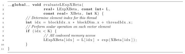
Listing 3.

Sparse CUDA kernel for updating Xβ, L × exp(Xβ), and M[L × exp(Xβ)] given X_j and Δβ_j

Exploiting Sparsity

Starting with Step (1) above, a very naive implementation recomputes the matrix-vector product at each cycle with complexity $\mathcal{O}$(KJ) and the potential to drive run-time to a dead-lock. Zhang and Oles (2001) and Wu et al. (2009) independently identify the savings that the one-dimensional update affords here. These works, along with Genkin et al. (2007), exploit the sparsity of X in updating the dense K-dimensional vector Xβ (Step 1). For comparison, these papers refer to Xβ as (r₁, … , r_N). However, we are unaware of others who continue to exploit the sparsity of X in moving from Xβ through to the subject-specific components of the gradient and Hessian (Steps 2 - 4).

With the numerator and denominator components of W in hand, we form a simple element-wise transformation and take two simultaneous inner products to return N’W and N’ [W × (1 – W)]. We discuss the advantages of these fused reductions for both host CPUs and GPUs shortly. This operation carries worst-case serial complexity $\mathcal{O}$(N) when all subjects have at least one exposure era that the current drug influences. Since several drugs carry prevalences among subjects nearing 25-50%, keeping track of the non-zero elements in W and performing sparse operations often reduces efficiency given the extra over-head and irregular memory access. In either case, the work in this fused-reduction is far greater than the work required to compute the one-dimensional gradient and Hessian contributions of the prior on β_j, so we leave the prior details to the reader. Finally, after cycling over all drugs j, we evaluate the convergence criterion. Whether one checks the change in Xβ (Genkin et al., 2007) or in the log-posterior, these computations remain a daunting $\mathcal{O}$(K). Fortunately, we only envoke them once per complete cycle and this task’s run-time becomes nearly irrelevant for moderate J.

Fine-Scale Parallelization

From these computational complexities, we immediately identify that Step (2) dominates run-time when X is dense at $\mathcal{O}$(K) and with a very large scalar constant. On the other hand, for sparse X, the fused reduction at $\mathcal{O}$(N) trumps run-time. Fortunately, these operations, along with the other update steps, are prime targets for parallelization using GPUs.

Code Listing 1 presents a basic CUDA kernel to perform the dense computation of Step (2). To envoke this kernel, the host program requests the short-lived execution of K threads, one for each computed element. Unlike coarser-scale parallelization using MPI across clusters or even multi-core approaches, the cost of creating and destroying threads is often negligible for GPUs; this makes such fine-scale parallelization ideal for embedding within serial algorithms. While each thread executes independently in this kernel as there is no shared data between threads, we still group threads into relatively large thread-blocks of size, say, 8 × 16 or 16 × 16. For all NVIDIA hardware, 16 sequential global memory read/writes “coalesce” into a single transaction, and the GPU interleaves the execution of multiple 16-thread sets in the same block to hide transaction latency. While recent GPUs relax the sequential requirement modestly, both processes significantly decrease memory-bandwidth limitations, improving arithmetic throughput. All of the work of this kernel falls in a single line of code. The theoretical complexity of this operation in parallel reduces to $\mathcal{O}$(1); however, in practice, one achieves $\mathcal{O}$(K/C) where C counts the number of GPU processing cores available to the host. This quantity can range from the low-10s on an integrated GPU in a mobile device or laptop to the mid-100s on a dedicated GPU card in a desktop through to the low-1000s on multiple GPU devices attached to a single host.

Listing 1.

Dense CUDA kernel for element-wise evaluation of L × exp(Xβ) given L and Xβ

Fused Operations

We turn our attention to the element-wise transformation and simultaneous inner products that provide a noteworthy example of effective optimization for massive datasets. Fusing these steps into a single operation avoids explicitly forming W, writing to its location in memory N times and then immediately reading from it N or 2N times, depending on if we perform the inner products simultaneously or separately, for each cycle step. Further, we only need to read from N once during the simultaneous reduction. This can significantly reduce memory bandwidth requirements on both the host CPU and GPU. Memory bandwidth measures the rate at which the processor can read data from or store data to memory. With increasingly faster processor speeds, many algorithms in statistics are memory bandwidth-limited rather than arthimetic throughput-limited. These optimization strategies fall under the name of “lazy evaluation” to “reduce temporaries” and warrant greater recognition among computational statisticians who provide high-performance tools. Modern computing language compilers are very proficient at optimizing away such intermediates for scalar operations, but often fail for vectors since large vectors cannot be held entirely in processor registers. For CPU-computing, high-level linear algebra libraries, such as Eigen, adeptly reduce the use of vector and matrix temporaries and provide lazy evaluation through “expression templates” (Veldhuizen, 1995). For the GPU, the Thrust library furnishes expression templates for fusing a univariate-to-univariate transformation and reduction of a single input vector, and we highly recommend this tool. However, currently, statisticians are hardpressed to find a GPU library that takes two input vectors, performs a bivariate-to-bivariate transformation and simultaneously reduces both output vectors. While such functionality may initially appear convoluted, it finds use in efficiently computing the one-dimensional gradient and Hessian for any GLM with minor modification to the transformation. To this end, we hand-craft our own.

Listing 2 presents our fused CUDA kernel. To envoke this kernel, the host program requests the execution of a moderate number (PARTIAL_SUM ≤ 64) of thread-blocks in which each block drives 256 or more (BLOCK_SIZE) threads depending on the hardware. In parallel, each thread begins by looping over N/(PARTIAL_SUM × BLOCK_SIZE) elements in M[L × exp(Xβ) × X_j], M[L × exp(Xβ)] and N, forming their transform and accumulating both inner product contributions for these elements. We interleave which elements each thread visits to coalesce memory transactions. Once completed, the threads within a block exploit the block’s shared memory to perform two generic $\mathcal{O}$(log BLOCK_SIZE) tree-based parallel reductions (Harris, 2010). While limited in quantity, shared memory on a GPU sports orders of magnitude faster access time than global memory and is accessible by all threads in the same block during their execution. Shared memory enables threads to conveniently share data, such as is required in the tree-reduction. The CUDA software development kit (SDK) furnishes several examples of tree-based parallel reductions. The output from this kernel are sets of partial-sums for g_j(β) and h_j(β), each of length PARTIAL_SUM ⪡ N. Instead of envoking a second round of parallel reduction on these partial-sums, we perform the final work in series on the host. Because of high communication latency between the host and GPU device, it takes comparable time to transfer 2 floating-point values as the modest 2 × PARTIAL_SUM. CPU/GPU work-balance will be a hallmark for speed-efficient statistical fitting of massive datasets.

Listing 2.

Fused CUDA kernel for transformation and reduction of numerators M[L × exp(Xβ) × X_j], denominators M[L × exp(Xβ)] and N to partial-sums of g_j(β) and h_j(β). Partial-sums end in length PARTIAL_SUM and we further reduce these on the host for efficiency. Function paralleReduction performs a generic logarithimic-order reduction in shared memory.

In terms of work-balance, while the fused reduction is the rate limiting step for sparse X on both the CPU and GPU, we can significantly decrease the communication latency between the host and GPU by additionally o -loading all of Steps (1) through (4) to the GPU well. Instead of uploading 2 × N floating-point numbers to the GPU in each cycle step, we succeed in reducing this number to a single floating-point Δβ_j. The cost, of course, is additional programming and the need for performing sparse operations on the GPU.

Representation in Memory

Memory access is often irregular for sparse linear algebra, and the computational statistician needs to pay particular attention to how both sparse matrices and vectors are represented in memory (Bell and Garland, 2009; Baskaran and Bordawekar, 2009). For example, the optimal representations for X and N differ. Only single columns of X enter into Steps (1) and (4) at a time, highlighting the need for compressed column storage (CCS) in which one places consecutive non-zero elements of each column X_j into adjecent memory addresses. While the standard representational choice for sparse-matrix/dense-vector (spMV) multiplication is compressed row storage (CRS), naive CRS representation of X would be detrimental to run-time on computing hardware with limited low-level caches, such as GPUs, since CRS is designed for row-by-row access. On the other hand, loading matrix M does enter into W as a spMV multiplication operation when X is dense, suggesting CRS. For sparse X, # (X_j) ⪡ # (M), so precomputing MX_j for all j in coordinate (COO) representation is simple and effective. COO representation consists of two index arrays, one to hold the row-indicators and one to hold the column-indicators of the non-zero entries, held in a third value array. Here the column-indicators of MX_j conveniently are the same as the column-indicators of X_j. Stored as a structure of arrays (SoAs), memory access to the row- and column-indicators is sequential, well-cached on the host CPU and coalesced on the GPU. However, retrieving the individual elements of L × exp(Xβ) remains irregular. Finally, the non-zero entries of both X and N are all one, so they need not be stored.

Executing an independent thread for each non-zero element of X_j to update M[L × exp(Xβ) X_j] may result in race conditions when multiple threads attempt memory transactions on the same elements in M[L × exp(Xβ) × X_j] in global memory. One solution entertains launching one or more cooperative threads tied to each of the N rows in MX_j. This may generate large inefficiencies as many rows in MX_j contain only zeros. Alternatively, the last few generations of GPUs contain small on-processor memory caches that enable relatively quick “atomic” transactions, in which only one thread may access a specific address in global memory at a time. This avoids race conditions and allows us to fuse the sparse updates of Steps (1) through (3) together into a single kernel. Listing 3 presents our sparse CUDA kernel to update Xβ, L × exp(Xβ), and M[L × exp(Xβ)] given Δβ_j. We envoke this kernel with one thread per non-zero entry in X_j, grouping threads into large blocks to help hide memory latency.

Precision

Graphics rendering traditionally requires at most 32-bit (single precision) floating-point computation to encompass 8-bits of red, green, blue and alpha. Ensuingly, GPU performance remains greatest at single precision. While the latest generations of GPUs can operate with 64-bit (double precision) numbers, the precision boost comes with a performance cost because the GPU contains fewer double precision arthimetic logical units, resulting in approximately half the maximum floating-point operations per second. Further, double precision mandates reading and writing twice as much information. For fitting the BSCCS model to massive datasets, single precision arthimetic suffices; the computations do not involve substracting approximately equal quantities, nor multiplying small quantities, both of which may lead to underflow. To demonstrate this point, finding ${\widehat{\beta }}_{\mathrm{MAP}}$ for BSCCS is a convex optimization problem (Simpson, 2011). Subsequently, h_j(β) < 0 and all elements of [W × (1 – W)] ≥ 0. Likewise, all elements of L, exp (Xβ) and, therefore, W ≥ 0.

2.5 Hyperparameter Selection and Measures of Coefficient Uncertainty

We aim to provide a full Bayesian analysis of all unknown parameters in our model. However, at present this remains beyond our computational limits. As a stopgap solution, we borrow two frequentist Monte Carlo proceedures. We learn about the hyperparameter σ² through a 10-fold cross-validation scheme. Previously, the computational cost of fitting the BSCCS model was too great to consider the hyperparameter as random, requiring an arbitrarily fixed value. Under this cross-validation scheme, we randomly separate the cases-only dataset into 10 portions, fit the BSCCS model via CCD on 10–1 of these portions and compute the predictive log-likelihood L (β) of the remaining portion given the fit. We repeat this process across a log-scale grid of hyperparameter values and chose the hyperparameter that maximizes the predictive log-likelihood. To moderately reduce the number of iterations required to acheive convergence of the CCD algorithm for successive hyperparameter values, we order the grid values from smallest to largest prior variance and exploit a series of “warm-starts.” At small variance under the Laplacian prior, most coefficients shrink to 0 and only slowly enter into the regression as the variance increases (Wu et al., 2009). Under the warm-start, the maximized regression coefficients from the previous fit serve as starting values for the next fit. In general, the predictive log-likelihood surface is relatively flat in the region around its maximum, so precise estimation of the hyperparameter is unnecessary. Alternative maximization strategies involving an initial bracketing of the maximized predictive log-likelihood and an intervaled line search often yield more precise estimates in fewer evaluations of the predictive log-likelihood.

Along with the infeasibility of estimating the hyperparameter, generating measures of uncertainty on the regression coefficients has remained taxing, to say the least, for the BSCCS model applied to massive observational databases. As a first attack at this problem, we examine the non-parametric bootstrap (Efron and Tibshirani, 1986) in the context of a L₁ regularized GLM (Park and Hastie, 2007). Procedures for generating standard errors for parameter estimates in the context of L₁ or L₂ regularization that are both computationally efficient and theoretically well-supported remain out of reach. The simple non-parametric bootstrap approach we pursue here has some short-comings (see Chatterjee and Lahiri (2011) for a related discussion in the context of linear regression), but we view it as a pragmatic approach pending a more complete solution. Without getting embroiled in this discussion, we report 95% confidence intervals derived from the 2.5% and 97.5% quantiles of 200 bootstrap samples. Under the Laplacian prior and as a “poor man’s estimate” of the posterior probability that β_j ≠ 0, we also report ${\widehat{p}}_j$ for each drug, the observed bootstrap proportion in which ${\widehat{\beta }}_j$ achieves a non-zero MAP estimate.

3 Demonstration

We examine the computational performance of fitting the BSCCS model across several large-scale observational databases and AEs. In particular, we show results from two medical claims databases and acute liver injury, acute renal failure, bleeding and upper gestrointestinal tract ucler hospitalization events in order to provide an examplar range of dataset sizes. Our results explore the effects of optimization and parallelization and are not meant here to identify medical products associated with these events. The MarketScan™ Commercial Claims and Encounters (CCAE) Research Database from Thomson Reuters is a large administrative claims database containing 59 million privately insured lives and provides patient-level deidentified data from inpatient and outpatient visits and pharmacy claims of multiple large employers. The MarketScan Lab Database (MSLR) contains 1.5 million persons representing a largely privately-insured population, with administrative claims from inpatient, outpatient, and pharmacy services supplemented by laboratory results. These databases constitute part of the data community established within the the Observational Medical Outcomes Partnership (OMOP). OMOP is a public-private partnership between government, industry and academia to conduct methodological research to inform the appropriate use of observational healthcare data for active medical product surveillance.

These example datasets span N = 115K to 3.6M cases-only patients taking J = 1224 to 1428 different drugs. The datasets provide K = 3.8M to 75M total (unique) exposure eras per analysis. We perform all benchmarking on the Amazon Elastic Compute Cloud, exploiting an Intel Xeon X5570 CPU @ 2.93GHz and one NVIDIA Tesla C2050. This GPU device sports 448 cores @ 1.15GHz. Performance on less expensive, commodity-grade GPUs, such as the NVIDIA GTX580, is often greater due to a slightly larger number of cores per GPU and higher memory-bandwidth. Due to data licensing agreements, however, we are restricted to Amazon hardware.

Figure 2 presents the relative speed-up our algorithms enjoy when inferring MAP estimates. These gains first compare implementing Steps 2 - 4 as sparse operations and then porting computing to the GPU. Sparsity generates up to a 181-fold speed-up; while the GPU multiplies this by up to another 37-fold. To put these times on an absolute scale, MAP estimation for our largest dataset originally drained over 51 hours; sparse operations on the GPU reduce this time to 29 seconds. Naturally, with fitting times standing in the 10s of hours, the hopes for cross-validation or bootstrap remain low, but grow very practical at 10s of seconds per replicate.

Figure 2.

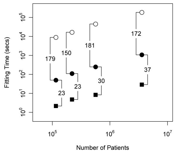
Maximum a posteriori estimation for several observational databases under the Bayesian self-controlled cases series model. We provide run-times for three implementations: dense computation on the CPU (white circles), sparse computation on the CPU (black circles) and sparse computation on the GPU (black squares).

Cross-validation to learn the hyperparameter σ² across these four datasets returns optimal variances ranging from 0.05 to 0.15 for L₁ and 0.02 to 0.13 for L₂. Importantly, these ranges are approximately an order-of-magnitude smaller than the arbitrary fixed value previously assumed in our BSCCS studies for drug surveillance. Employing the optimal hyperparameter, Figure 3 reports non-parameteric bootstrap confidence intervals of drug effects for a single representative dataset under the L₁ prior. This dataset explores angioedema events within the CCAE database and contains N = 76K case-only patients, taking J = 1162 drugs and yielding K = 2.1M exposure eras. In the figure, we first rank all drugs by their MAP estimate ${\widehat{\beta }}_j$ in decreasing order and then plot the 95% confidence intervals for the 441 drugs for which ${\widehat{p}}_j$ > 0.50. Darker interval shading reflects larger ${\widehat{p}}_j$. While a general trend holds in which larger $\mid {\widehat{\beta }}_j\mid$ more often return 95% confidence intervals that do not cover 0, we identify notable exceptions. Namely, Drotrecogin alfa, an anti-thrombotic, anti-inflammatory agent used in the treatment of severe sepsis, returns with the fourth largest effect estimate, but its confidence interval continues to cover 0, reflecting the high sampling variability in this estimate.

Figure 3.

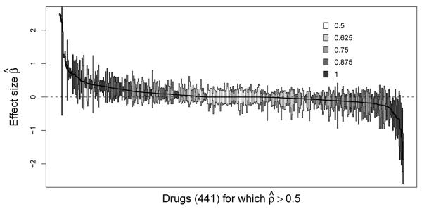
Exemplar uncertainty analysis of angioedema as an adverse event under the L₁ prior. Here, we plot the non-parametric bootstrap 95% confidence intervals for the 441 drug effects that demonstrated non-zero coefficients in at least 50% of the bootstrap replicates. Gray-scaling reports the proportion of bootstrap replicates in which effect estimates are non-zero.

4 Discussion

Efficient algorithmic design and massive parallelization open the door for fitting complex GLMs to massive datasets. Computational statisticians regularly capitalize on the sparsity of their model and data, and this is an important design issue for the BSCCS we consider here, since the design matrix X consists purely of sparse covariates. In particular, we identify that the sparsity of X carries all the way through to computing the subject-specific contributions to the model gradient and Hessian, resulting in over a 100-fold speed-up compared to the most advanced CCD algorithms for GLMs of which we are aware. Many GLMs, however, command dense covariates as well, such as baseline measurements, and other techniques become necessary. Here fusing multiple transformations and reduction together into vectorizable kernels is the first step in off-loading the work to the GPU, and we hope our discussion in this paper raises awareness of these techniques among computational statisticians. The end result for the BSCCS model is an approximate 30-fold speed-up on a single GPU compared to a single CPU core. These techniques also port directly to utilizing multi-core CPUs and multiple GPUs simultaneously, although we do not explore this avenue in this paper to simplify comparisons.

Advancing model complexity is both possible in the sampling density of the data and in the prior assumptions on the unknown model parameter. Here we have only considered independent and identically distributed prior densities over the drug effect sizes. More biologically plausible hierarchical distributions are conveniently available. For example, to borrow strength, we may favor grouping drugs a priori into classes based on mode of action or therapeutic targets. Similarly, we may wish to explore borrowing strength across related outcomes. Because computation of the prior gradient and Hessian remains extremely light-weight, no modification to the GPU code is necessary and run-times should remain as quick.

One immediate advantage of the orders-of-magnitude reduction in run-time stands the ability to nest point-estimation within both cross-validation and bootstrap frameworks, making these Monte Carlo frameworks feasible. Cross-validation and bootstrapping begin to allow us to estimate model hyperparameters and report measures of uncertainty around the usual point-estimates. For the drug surveillance community, this represents a giant leap forward. For example, most of the statistial methods in OMOP are implemented in the statistical packages SAS or R (http://omop.fnih.org/MethodsLibrary). One of our own preliminary implementations of the BSCCS model in R, using just a sparse matrix package and no further linear algebra libraries, requires around 5.3 hours to generate a single MAP estimate from a dataset with only N = 7460. With this benchmark in mind, it is no wonder why almost all computationally expensive fitting of massive datasets in the field has ignored cross-validation and bootstrapping; see, e.g., Funk et al. (2011), and a presentation at the 2011 International Congress on Pharmacoepidemiology involving a similar study redoubled this point by claiming that bootstrapping is computationally infeasible with more than 20K patients. High performance statistical computing involving massive parallelization shows that these limitations are quickly lifting.

We achieve this success by exploiting the GPU within a serial CCD algorithm. CCD is a generic optimization approach and we envision extensions working for massive dataset applied to models beyond the GLM setting as well. Moving past CCD, Zhou et al. (2010) consider similar block-relaxation and majorization techniques to attack large-scale matrix factorization and multidimensional scaling using GPUs. Here and in CCD, one breaks a high-dimensional optimization problem into a series of low-dimensional updates that involve many scalar operations. As Zhou et al. (2010) demonstrate with their quasi-Newton acceleration application, one ideally aims for one-dimensional updates, as even slightly higher-dimensional operations carry heavy data-dependency that can outweigh the advantages of the GPU.

To accomplish parallelization within a serial algorithm, we take advantage of the wide vector-processing capabilities of the GPU to perform simple operations simultaneously across a large input of data. This vectorization lacks branches in the kernel code, avoiding thread divergence and serialization of the work within the wide vector. As a result, expected speed-up scales most directly with the quantity of data. This differs considerably from distributing EP tasks, such as those that arise in many Monte Carlo approaches including the independent and often divergent particle evolution in a sequential Monte Carlo, to separate cores of the GPU. Here, we receive at little cost more particles and higher precision estimates with additional cores. Unfortunately, however, this strategy loses out on scaling in the critical dimension of the data as massively parallel devices continue to mushroom in size.

References

- Baskaran M, Bordawekar R. Optimizing sparse matrix-vector multiplication on GPUs. IBM research report RC24704. 2009.
- Bell N, Garland M. Efficient sparse matrix-vector multiplication in CUDA. Proc. ACM/IEEE Conf. Supercomputing (SC), Portland; OR, USA. New York: ACM; 2009. [Google Scholar]
- Chatterjee A, Lahiri S. Bootstrapping lasso estimators. Journal of the American Statistical Association. 2011;106:608–625. [Google Scholar]
- Coplan P, Noel R, Levitan B, Ferguson J, Mussen F. Development of a framework for enhancing the transparency, reproducibility and communication of the benefit–risk balance of medicines. Clinical Pharmacology & Therapeutics. 2011;89:312–315. doi: 10.1038/clpt.2010.291. [DOI] [PubMed] [Google Scholar]
- Curtis J, Cheng H, Delzell E, Fram D, Kilgore M, Saag K, Yun H, Du-Mouchel W. Adaptation of Bayesian data mining algorithms to longitudinal claims data: coxib safety as an example. Medical care. 2008;46:969–975. doi: 10.1097/MLR.0b013e318179253b. [DOI] [PMC free article] [PubMed] [Google Scholar]
- Dennis J, Jr, Schnabel R. A view of unconstrained optimization. Handbooks in operations research and management science. 1989;1:1–72. [Google Scholar]
- d’Esopo D. A convex programming procedure. Naval Research Logistics Quarterly. 1959;6:33–42. [Google Scholar]
- Efron B, Tibshirani R. Bootstrap methods for standard errors, confidence intervals, and other measures of statistical accuracy. Statistical Science. 1986;1:54–75. [Google Scholar]
- Farrington C. Relative incidence estimation from case series for vaccine safety evaluation. Biometrics. 1995;51:228–235. [PubMed] [Google Scholar]
- Funk M, Westreich D, Wiesen C, Stürmer T, Brookhart M, Davidian M. Doubly robust estimation of causal effects. American journal of epidemiology. 2011;173:761–767. doi: 10.1093/aje/kwq439. [DOI] [PMC free article] [PubMed] [Google Scholar]
- Genkin A, Lewis D, Madigan D. Large-scale Bayesian logistic regression for text categorization. Technometrics. 2007;49:291–304. [Google Scholar]
- Harris M. Optimizing parallel reduction in CUDA. 2010. nVidia, online.
- Jin H, Chen J, He H, Williams G, Kelman C, O’Keefe C. Mining unexpected temporal associations: Applications in detecting adverse drug reactions. Information Technology in Biomedicine, IEEE Transactions on. 2008;12:488–500. doi: 10.1109/TITB.2007.900808. [DOI] [PubMed] [Google Scholar]
- Kulldorff M, Davis R, Kolczak M, Lewis E, Lieu T, Platt R. A maximized sequential probability ratio test for drug and vaccine safety surveillance. Sequential Analysis. 2011;30:58–78. [Google Scholar]
- Kyung M, Gill J, Ghosh M, Casella G. Penalized regression, standard errors, and Bayesian lassos. Bayesian Analysis. 2010;5:369–412. [Google Scholar]
- Lange K. A gradient algorithm locally equivalent to the EM algorithm. Journal of the Royal Statistical Society, Series B. 1995;57:425–437. [Google Scholar]
- Lee A, Yau C, Giles M, Doucet A, Holmes C. On the utility of graphics cards to perform massively parallel simulation of advanced Monte Carlo methods. Journal of Computational and Graphical Statistics. 2010;19:769–789. doi: 10.1198/jcgs.2010.10039. [DOI] [PMC free article] [PubMed] [Google Scholar]
- Li L. A conditional sequential sampling procedure for drug safety surveillance. Statistics in medicine. 2009;28:3124–3138. doi: 10.1002/sim.3689. [DOI] [PubMed] [Google Scholar]
- Madigan D, Ryan P, Simpson S, Zorych I. Bayesian methods in pharmacovigilance. In: Bernardo J, Bayarri M, Berger J, Dawid A, Heckerman D, Smith A, West M, editors. Bayesian Statistics 9. Oxford University Press; Oxford, UK: 2011. pp. 421–438. [Google Scholar]
- Nelder J, Wedderburn R. Generalized linear models. Journal of the Royal Statistical Society. Series A (General) 1972;135:370–384. [Google Scholar]
- Norén G, Bate A, Hopstadius J, Star K, Edwards I. Temporal pattern discovery for trends and transient effects: its application to patient records. Proceeding of the 14th ACM SIGKDD international conference on Knowledge discovery and data mining; ACM, New York. 2008. pp. 963–971. [Google Scholar]
- Park M, Hastie T. L1-regularization path algorithm for generalized linear models. (Series B).Journal of the Royal Statistical Society. 2007;69:659. [Google Scholar]
- Ryan P, Suchard M, Madigan D. Learning from epidemiology: a framework for interpreting large-scale observational database studies Under review. 2012.
- Schneeweiss S, Rassen J, Glynn R, Avorn J, Mogun H, Brookhart M. Epidemiology. Vol. 20. Cambridge, Mass; 2009. High-dimensional propensity score adjustment in studies of treatment effects using health care claims data; pp. 512–522. [DOI] [PMC free article] [PubMed] [Google Scholar]
- Silberstein M, Schuster A, Geiger D, Patney A, Owens J. Efficient computation of sum-products on GPUs through software-managed cache. Proceedings of the 22nd Annual International Conference on Supercomputing; ACM, New York. 2008. pp. 309–318. [Google Scholar]
- Simpson S. Ph.D. thesis. COLUMBIA UNIVERSITY; 2011. Self-controlled methods for postmarketing drug safety surveillance in large-scale longitudinal data. [Google Scholar]
- Stang P, Ryan P, Racoosin J, Overhage J, Hartzema A, Reich C, Welebob E, Scarnecchia T, Woodcock J. Advancing the science for active surveillance: rationale and design for the observational medical outcomes partnership. Annals of internal medicine. 2010;153:600–606. doi: 10.7326/0003-4819-153-9-201011020-00010. [DOI] [PubMed] [Google Scholar]
- Suchard M, Rambaut A. Many-core algorithms for statistical phylogenetics. Bioinformatics. 2009;25:1370–1376. doi: 10.1093/bioinformatics/btp244. [DOI] [PMC free article] [PubMed] [Google Scholar]
- Suchard M, Wang Q, Chan C, Frelinger J, Cron A, West M. Understanding GPU programming for statistical computation: Studies in massively parallel massive mixtures. Journal of Computational and Graphical Statistics. 2010;19:419–438. doi: 10.1198/jcgs.2010.10016. [DOI] [PMC free article] [PubMed] [Google Scholar]
- Tibbits M, Haran M, Liechty J. Parallel multivariate slice sampling. Statistics and Computing. 2011;21:415–430. [Google Scholar]
- Tibshirani R. Regression shrinkage and selection via the lasso. Journal of the Royal Statistical Society, Series B. 1996;58:267–268. [Google Scholar]
- Veldhuizen T. Expression templates. C++ Report. 1995;7:26–31. [Google Scholar]
- Warga J. Minimizing certain convex functions. Journal of the Society for Industrial and Applied Mathematics. 1963;11:588–593. [Google Scholar]
- Wilkinson D. Parallel Bayesian computation. In: Kontoghiorghes E, editor. Handbook of Parallel Computing and Statistics. Chapman & Hall/CRC; New York: 2006. pp. 481–512. [Google Scholar]
- Wu T, Chen Y, Hastie T, Sobel E, Lange K. Genome-wide association analysis by lasso penalized logistic regression. Bioinformatics. 2009;25:714–721. doi: 10.1093/bioinformatics/btp041. [DOI] [PMC free article] [PubMed] [Google Scholar]
- Wu T, Lange K. Coordinate descent algorithms for lasso penalized regression. The Annals of Applied Statistics. 2008;2:224–244. doi: 10.1214/10-AOAS388. [DOI] [PMC free article] [PubMed] [Google Scholar]
- Zhang T, Oles F. Text categorization based on regularized linear classification methods. Information Retrieval. 2001;4:5–31. [Google Scholar]
- Zhou H, Lange K, Suchard M. Graphics processing units and high-dimensional optimization. Statistical Science. 2010;25:311–324. doi: 10.1214/10-STS336. [DOI] [PMC free article] [PubMed] [Google Scholar]