

Abstract
Recent research indicates that knowledge about social networks can be leveraged to increase efficiency of interventions (Valente, 2012). However, in many settings, there exists considerable uncertainty regarding the structure of the network. This can render the estimation of potential effects of network-based interventions difficult, as providing appropriate guidance to select interventions often requires a representation of the whole network. In order to make use of the network property estimates to simulate the effect of interventions, it may be beneficial to sample networks from an estimated posterior predictive distribution, which can be specified using a wide range of models. Sampling networks from a posterior predictive distribution of network properties ensures that the uncertainty about network property parameters is adequately captured. The tendency for relationships among network properties to exhibit sharp thresholds has important implications for understanding global network topology in the presence of uncertainty; therefore, it is essential to account for uncertainty. We provide detail needed to sample networks for the specific network properties of degree distribution, mixing frequency, and clustering. Our methods to generate networks are demonstrated using simulated data and data from the National Longitudinal Study of Adolescent Health.
1 Introduction
We develop a method to sample networks given a specification of the probability distribution– of particular interest is a posterior predictive distribution–on network statistics as researchers are often interested in utilizing observed network data to investigate the impact of an intervention on populations with networks similar to those for which the data are available. The probability distribution can be specified either by a posterior predictive model, design-based inference, Null model (e.g. the Erdős-Rényi model), or Bayesian inference for an exponential random graph model (ERGM) (Caimo & Friel, 2011; Koskinen et al., 2013). Methods to generate networks are widely available, and include those to generate networks based on one specific network property, such as the Erdős-Rényi model (Erdős & Rényi, 1960) and the Barabási-Albert model (Barabasi & Albert, 1999), as well as those that are based on a wide range of network properties, such as the simulation methods (Handcock et al., 2012) from an ERGM (Frank & Strauss, 1986). However, none of these network generation efforts incorporate uncertainty due to sampling and collection error. In the Erdős-Rényi model, the number of edges follows a binomial distribution with parameters .5n(n − 1) and p, where n is the number of nodes and p is the probability of an edge. ERGMs fix the probability distribution of network properties by maximizing the entropy (Newman, 2010). This paper connects the two research areas, modeling posterior predictive distributions and generating networks, by presenting a novel method for sampling networks from a user–defined posterior predictive distribution, thereby ensuring that the networks are consistent with not only point estimates but also their associated uncertainty. The properties we consider are density, degree distributions, mixing patterns and clustering, but these methods could be generalized to include many others.
Erdős & Rényi (1960) demonstrated the importance of characterizing the uncertainty in estimates of network properties by analytically relating the size of the largest component of an Erdős-Rényi graph to its expected mean degree. This work revealed the existence of sharp thresholds in relationships among network properties. Subsequent research has shown threshold behavior in the relationship between mean degree and categorization of networks as connected, Hamiltonian, or planar, along with relationships between mean degree and size of the largest clique and the network diameter under the Erdős-Rényi random graph model (Friedgut & Kalai, 1996). Watts & Strogatz (1998), in their landmark paper, demonstrated the rapid emergence of the small world property via changes in the mixing patterns between near and distant nodes. The tendency for network properties to exhibit sharp threshold effects – causing their joint distributions to be peaked (Newman, 2010) – demonstrate that slight errors in estimation of a network property can have a major impact on beliefs about the overall structure of the network. Therefore, it is essential for researchers to utilize knowledge about the variability of network property estimates.
Our approach allows for specification of the error distributions of the estimated network property or properties of interest and not just the estimate of the mean by the specification of a posterior predictive distribution. For a simple illustration, assume we collected sample data from an unknown network of interest, G, of size n. Let p̂ represent the point estimate for network edge density–the sole network property under consideration in this example. Regardless of whether the Erdős-Rényi model or the ERGM is used to generate a collection of networks, the probability distribution of network edge density for the collection of networks is approximately normal with mean p̂ and variance . However, the uncertainty in the estimated edge density depends on the number of units sampled and other sample design considerations. Furthermore, the error distribution may be non-normal. Our proposed method allows users to specify the posterior predictive distribution for edge density. Characterizing and incorporating uncertainty is particularly important when point estimates of network properties are near threshold values. The focus of the paper is on methods for generating a collection of networks given the specification of the probability distribution of network properties. The specification can be established either by a posterior predictive model, design-based inference, or a Null model, e.g. the Erdős-Rényi model.
To demonstrate our methods, we consider two settings with different types of observed network data but a common goal: the generation of collections of networks that represent new populations but retain the essential network properties inferred from the observed data. In the first setting, the observed data arise from a population-based sample of nodes. Such data have been analyzed to investigate the impact of concurrency on HIV propagation in the United States (Morris et al., 2009) and changes in the core-dependence network (including measures of social isolation) in the United States over a 20-year period (McPherson et al., 2006). Section 5 presents a simulation study that emulated the first setting by randomly sampling nodes from a network, and generating networks based on information from the samples. In the second setting, the observed data are a collection of whole networks. In this setting, the posterior predictive distribution incorporates the variation in network properties across the observed networks. Settings in which analysis of multiple networks is of interest include cluster randomized trials of interventions designed to prevent HIV infection (Wang et al., in press; Boily et al., 2012) or smoking initiation (Valente et al., 2003). They also include observational studies, such as those investigating impact of friendship network structure on adolescent development (McNeely et al., 2002). Section 6 analyzes data from The National Longitudinal Study of Adolescent Health (Add Health) on multiple friendship networks in order to simulate such networks in a hypothetical collection of schools that reflect the diversity of those actually studied.
Beyond the relative ease of collecting relevant data for their estimation, the network properties of degree distribution, mixing patterns and clustering provide necessary and often sufficient information to reconstruct networks in many settings (Mahadevan et al., 2006). Additionally, these properties have great influence on processes operating on networks. For example, the importance of mixing patterns, including age, social position, geographic location and race, has been studied in many settings, in particular sexual disease transmission (Morris et al., 2007). Degree mixing has also been important in many settings, including investigation of disease transmission models (Newman, 2002), the Internet (Doyle et al., 2005; Vázquez et al., 2002), and biological interactions (Maslov & Sneppen, 2002). Newman (2002) concluded that degree assortative networks disseminate disease more easily and are more robust to removal of their highest degree nodes compared to disassortative networks. Clustering is relevant in a wide range of network types including social, information, technological, and biological (Newman, 2010). Hence our focus is on degree distribution, mixing patterns and clustering; the discussion section addresses extension to additional network properties. An R package called CCMnet1 contains many of the methods presented in this paper.
The proposed methods permit generation of collections of networks, which facilitates simulation of processes on many probable realizations of a population that are consistent with estimates of network properties, and thereby permits characterization of the reliability of the conclusion. For example, a large collection of friendship networks that are based on observed networks available in the Add Health dataset can be useful to model and evaluate smoking prevention programs since an individual's propensity to smoke is influenced by his/her peers (Christakis & Fowler, 2008). Examples of research utilizing network collections include investigation of disease control strategies for Mycoplasma pneumoniae in hospitals (Bansal et al., 2006), influenza vaccination programs within an urban population (Meyers et al., 2003), and management of tuberculosis progression within an HIV infected population (Mills et al., 2011). Collections of networks have also been used to study factors that account for differences in prevalence of sexually transmitted diseases among groups (Morris et al., 2009) and the benefit of test and treat strategies to control HIV in Sub-Saharan communities (Palombi et al., 2012). However, none of the examples incorporate the full uncertainty in network property estimates; the models used to generate the networks are based only on mean values for network properties.
The next section provides a general description of the proposed method for generating network collections. Section 3 provides additional detail for categories of network collections that are of general interest. Section 4 describes how the proposed network generation method can be used to sample networks from a posterior predictive distribution. Sections 5 and 6 provide examples of sampling networks from a posterior predictive distribution for simulated data and data from The National Longitudinal Study of Adolescent Health (Add Health), respectively; and section 7 discusses the proposed methods and suggests future research directions.
2 Network Collection Properties
To describe the method for generating network collections requires defining terminology and notation. Let vector D(g) denote the degree distribution of a graph g, where the ith entry of D(g), Di(g), is the proportion of nodes with degree i. Let d(g) represent the degree sequence of network g, where the ith entry, di(g), is the degree of node i. Let MM(g) be a matrix representing the mixing pattern of graph g. The entry MMk,l(g) is the proportion of edges from a node with covariate pattern k to a node with covariate pattern l. Let vector m(g) represent the covariate pattern for each node in g, where mi(g) is the covariate pattern for node i. Let M(g) be the vector of proportions for the different covariate patterns. We use the notation DMM(g) to represent degree mixing matrices, where entry DMMi , j(g) is the proportion of edges from a node of degree i to a node of degree j. Finally, let CC(g) denote the clustering coefficient of g as described in Newman (2010).
The network collection is a subset of networks from the space,
 of graphs with n nodes. To generate such a collection, we begin by partitioning
into congruence classes, such that each network in the congruence class has the same values for network properties of interest. Let Cg represent the congruence class containing network g; and let the number of networks in Cg be denoted as |Cg|, also referred to as the volume factor in Shalizi & Rinaldo (2013). For example if interest lies in degree distribution and degree mixing patterns, networks g and h will reside in the same congruence class if and only if D(g) = D(h) and DMM(g) = DMM(h). The congruence classes represent the finest partition of the space
that is based on estimable quantities from observed data and is of scientific interest. In this paper, the congruence classes will be constructed by partitioning
by density, degree distribution, mixing patterns and clustering coefficient. To generate a collection, each network in
will be assigned a probability, P(g), of being selected into the collection. P(g) is based solely on the congruence class of the network g.
of graphs with n nodes. To generate such a collection, we begin by partitioning
into congruence classes, such that each network in the congruence class has the same values for network properties of interest. Let Cg represent the congruence class containing network g; and let the number of networks in Cg be denoted as |Cg|, also referred to as the volume factor in Shalizi & Rinaldo (2013). For example if interest lies in degree distribution and degree mixing patterns, networks g and h will reside in the same congruence class if and only if D(g) = D(h) and DMM(g) = DMM(h). The congruence classes represent the finest partition of the space
that is based on estimable quantities from observed data and is of scientific interest. In this paper, the congruence classes will be constructed by partitioning
by density, degree distribution, mixing patterns and clustering coefficient. To generate a collection, each network in
will be assigned a probability, P(g), of being selected into the collection. P(g) is based solely on the congruence class of the network g.
By partitioning
into congruence classes and defining a probability mass function for the probability of sampling a network from a congruence class, we can control the probability of sampling a network with particular values of network properties. As some congruence classes have vastly more networks than do others, this approach guards against over- or under-representing networks with particular properties due to the size of the congruence class, thereby ensuring the consistency of the collection of networks with the collected data. Defining the probability of sampling networks from a congruence class allows for generation of networks that reflect both the estimated mean and uncertainty associated with the estimate–the only information available to the investigator–without requiring consideration of the complex topology of the underlying space of graphs of size n.
A Markov chain Monte Carlo (MCMC) procedure is the basis for generating a collection of networks, {g1, … ,gt} that satisfy the probability distribution assigned to the congruence classes. Ideally, to generate our collection, {g1, … ,gt}, we would sample, with replacement, t congruence classes {C1, … ,Ct}, based on the probability distribution on the classes. For each congruence class, Ci where i ∈ {1, … ,t}, we would draw a network, gi, such that gi ∈ Ci. Since this procedure presents computational difficulties, we implement a Markov chain using the Metropolis-Hastings algorithm to generate the networks. For a review on MCMC methods see Robert & Casella (2004). In order to implement the Metropolis-Hastings algorithm, four aspects have to be specified: target function, proposal function, acceptance probability, and initial starting element. Many authors have described construction of an initial starting element (Blitzstein & Diaconis, 2010), so we discuss only the first three aspects below.
2.1 Target Function
The target function is the desired stationary distribution for the Markov chain. In our setting, the network g has a probability mass equal to the probability of the congruence class Cg divided by the number of networks in Cg, |Cg|, thereby ensuring that each network in Cg has the exact same probability:
| (1) |
Due to the constraints imposed on particular network properties, not all values of particular network properties correspond to valid networks. For example, no network can have odd values for Σi Di × i × n, which represents two times of the number of edges in the graph. Section 3 outlines criteria to ensure that a congruence class contains at least one valid network.
2.2 Proposal Function
The algorithm generates the next network, gt+1, in the chain by nominating a proposal network, gpt+1, based only on the previous network gt. A common method to generate a proposal network is by toggling the existence of an edge. Edge toggling requires selecting two nodes at random and either removing the edge if one exists or adding one if it does not. The algorithm produces an irreducible Markov chain among all graphs with a fixed size; the chain also has equal forward and backward probabilities.
2.3 Acceptance Probability
Once a proposal network, gpt+1, is generated, the Metropolis-Hastings algorithm will either accept, gt+1 = gpt+1, or reject, gt+1 = gt, the proposal. The Metropolis-Hastings acceptance probability is the following:
| (2) |
Let t(g, Ch) equal the number of elements in Ch that differ from g through toggling one edge. Let represent the total number of possible edge toggles for graphs in Cg to graphs in Ch. Due to symmetry induced by edge toggling, T(Cg, Ch) = T(Ch,Cg). Thus,
| (3) |
By defining f(Cg, Ch) as the average number of elements in Ch that are valid proposals from an element g ∈ Cg, we get the following:
| (4) |
3 Network Collection Generation
This section demonstrates our framework by considering several common scenarios. Once the network space and network proposal method have been selected, only the functions PC(Cg) and f(Cg,Ch) need to be specified. In all scenarios, the network space consists of all networks with a fixed number of nodes; edge toggling is used to propose networks. As the probability mass function, PC, on congruence classes is set by the investigator, in this section we only derive f(Cg, Ch). Sections 5 and 6 provide examples of various probability mass functions associated with different sampling strategies. Denote g, h ∈
as the current and proposal network, respectively. Let Cg and Ch denote the congruence classes for g and h. Let the edge, (i, j), between node i and node j be the connection that is toggled to move from g to h and back. Without loss of generality, let (i, j) ∈ h but (i, j) ∉ g.
3.1 Topological Properties
Topological properties of a social network provide valuable insight into the operation of processes within a community. This section discusses generation of networks based on density, degree distribution, degree assortativity, and clustering. Though density is an influential network property (Bollobás, 2001), it is usually collected with other network properties, e.g. degree distribution, but it provides a useful example to illustrate the mechanics of the proposed method.
3.1.1 Density
For density, a congruence class is the set of networks with the same number of edges, as all graphs in
have the same number of nodes. Let |Eg| denote the number of edges in graph g. Networks g1 and g2 are in the same congruence class if and only if |Eg1| = |Eg2|. Since (i, j) ∈ h but (i, j) ∉ g, |Eh| = |Eg| + 1. To calculate f(Ch,Cg) we need to know the average number of elements in Cg that are valid proposals from any element h ∈ Ch. Since removing any edge in h will produce a graph in Cg there are exactly |Eh| valid proposals in Cg from graph h, and this is true regardless of the choice of h ∈ Ch. Thus,
| (5) |
To calculate f(Cg,Ch), we need to know the average number of elements in Ch that are valid proposals from any element g ∈ Cg. Adding a new edge in g that did not previously exist will produce a graph in Ch; hence, there are exactly valid proposals in Ch from graph g. Again, is it true for any g ∈ Cg. Thus,
| (6) |
The investigator can stipulate the proportion of networks in the collection with a particular number of edges by specifying the values of P(Cg). One choice of specification is to generate a network collection following Erdős-Rényi random graph model with parameters (n, p); this can be achieved by setting . Another specification, which is a major goal of this paper, is to define P(Cg) in such a way to generate networks based on the uncertainty due to sampling.
3.1.2 Degree Distribution
For degree distribution, congruence classes are sets of networks with identical numbers of nodes and degree distribution. Thus, networks g1 and g2 are in the same congruence class if and only if Dk(g1) = Dk(g2) ∀ k. As g only differs from h through a toggling of the edge (i, j), Dk(g) = Dk(h) for all k except possibly k = di(g), dj(g), di(h) and dj(h). Since the only difference between the graph g and h is edge (i, j) ∈ h but (i, j) ∉ g, di(h) = di(g) + 1 and dj(h) = dj(g) + 1. The expressions relating D(g) and D(h) are given below for those entries that may differ:
| (7) |
The number of edge toggles from a graph h ∈ Ch to any graph in Cg is equal to the proportion of edges in h that have endpoint degrees of di(h) and dj(h), i.e. DMMdi(h), dj(h), multiplied by the number of edges in h, |Eh|. Thus, f(Ch,Cg) is equal to the average of DMMdi(h), dj(h) × |Eh|over all graphs h ∈ C. Let E(DMM|Ch) denote the expected degree mixing matrix over graph that are in Ch. Since h′ ∈ Ch if and only if D(h′) = D(h),E(DMM|Ch) = E(DMM|D(h)). Thus,
| (8) |
Following arguments from Newman (2002), based on the probability that a node's neighbor will have degree k is proportional to kDk and not Dk,
| (9) |
The number of edge toggles from a graph g ∈ Cg to any graph in Ch is equal to the number of possible non-loop edges with endpoint degrees di(g) and dj(g) minus the number of edges that will generate a multi-edge. The expected number of edge toggles that generate a multi-edge is E(DMMdi(g), dj(g) |D(g)) × |Eg|,denote this value as α1; therefore, an expression for f(Cg, Ch) is the following,
| (10) |
To decrease convergence time in the MCMC procedure, one can use the algorithm described in Blitzstein & Diaconis (2010) to initialize the starting network with the estimated mean degree distribution. Based on results from Hakimi (1962) and Havel (1955), an algorithm to validate that a degree sequence has a realization can be found in Blitzstein & Diaconis (2010).
3.1.3 Degree Mixing and Degree Distribution
We consider a partition of
such that networks g1 and g2 are in the same congruence class if and only if Dx(g1) = Dx(g2) ∀x and DMMx,y(g1) = DMMx,y(g2) ∀x,y. An identical partition is defined when networks g1 and g2 are in the same congruence class if and only if DMM(g1)|Eg1| = DMM(g2)|Eg2|. Thus, the probability mass function can be defined using the degree mixing matrix and number of edges.
Toggling the edge (i,j) in a graph h ∈ Ch, not only changes the entry associated with index (di(h),dj(h)) in DMM(h), but also changes the set of entries associated with indices {(di(h),dk(h))}k∈{in } and {(dl(h), dj(h))}l∈{jm} where and denote the set of neighbors of i and j, respectively. Therefore, to move from a graph h ∈ Ch to any graph in Cg via edge toggling, an edge (i, j) with the proper degrees for i and j as well as the proper degrees for the neighbors of i and j needs to be toggled. Let di and dj denote the proper degrees for i and j to move from a graph h ∈ Ch to any graph in Cg. Additionally, let {din} and {djm} denote the proper degrees of the neighbors of i and j, respectively. f(Ch,Cg) is the average over all graphs in Ch of the number of edges with endpoint degrees of di and dj, and neighbors with degrees {din} and {djm} The expression for f(Ch,Cg) in the degree mixing case is similar to the expression for degree distribution, as shown in equation (8), except for an extra term for the probability that an edge with degrees di (h) and dj (h) has neighbors with the proper degrees. f(Ch,Cg) is equal to DMMdi(h), dj(h) × |Eh| multiplied by the probability that an edge with endpoint degrees equal to di and dj has neighbors with degrees equal to {din} and {djm}; let denote this probability. Therefore,
| (11) |
When removing any edge, (i,j), from h with endpoint degrees of di (h) and dj (h), it is known that one of the di (h) neighbors of i has degree dj (h) and one of the dj (h) neighbors of j has degree di (h). However, when adding any edge, (i, j), with particular endpoint degrees to g none of the degrees of the neighbors of i or j are known. Therefore, the probability that an edge with endpoint degrees equal to di and dj has neighbors with degrees equal to {din} and {djm}has a slightly different expression for the two transitions, Ch to Cg and Cg to Ch. Let denote the probability that an edge with degrees di(g) and dj (g) has neighbors with the proper degrees when transitioning from Cg to Ch. The expression for f(Cg,Ch), which is similar to the expression (10) for degree distribution, is the following,
| (12) |
where α2 = DMMdi(g),dj(g)(g) × |Eg|.
is equal to the average over all graphs in Cz of the number of ways to select edges adjacent to i and j with endpoint degrees of {(din, di)} and {(djm, dj)} divided by the total number of possible ways to select edges adjacent to i and j. Let the entries of DMM′ (z) × |Ez| contain the total number of half edges, i.e. stubs; the entry DMM′k,l(z) × |Ez| is the number of stubs from a node of degree k that attaches to a node of degree l. Therefore, if k≠l and if k = l. The number of ways to select m half edges each with an endpoint degree of k and attaches to a node of degree l is . The number of ways to select edges adjacent to i and j with proper endpoint degrees is approximately the product of the number of ways to select the necessary number of stubs over each distinct endpoint degree. The product only needs to be indexed over degrees that exist in {di (z), dj (z)}, since the edges connect to i or j and the degrees of i and j are known. The denominator of is equal to the number of ways to choose valid stubs for the neighbors of i and j from the total number of valid stubs that attach to nodes with degrees equal to di or dj. When transitioning from h to g it is known that i and j are neighbors, thus only di − 1 and dj − 1 neighbor degrees need to be specified for i and j, respectively. The formula for is the following,
| (13) |
where and denote the number of elements in {din} and {djm} equal to k.
As with the degree distribution, not all degree mixing matrices have a valid realization. Appendix A provides a method to characterize valid degree mixing matrices; an alternative proof of the validity of this characterization is given by Amanatidis et al. (2008). Using the construction procedure in the appendix to set the initial network with the estimated degree distribution and degree mixing will tend to decrease time to convergence in the MCMC procedure.
3.1.4 Degree Distribution, Degree Mixing, and Clustering
We consider a partition of
such that networks g1 and g2 are in the same congruence class if and only if Dx(g1) = Dx(g2)∀ x, DMMx,y(g1) = DMMx,y(g2)∀ x,y, and CC(g1) = CC(g2). An identical partition is defined when networks g1 and g2 are in the same congruence class if and only if DMM(g1)|Eg1| = DMM(g2)|Eg2| andT(g1) = T(g2), where T (g) is the number of 3-cycles in g. Let
represent the average number of elements in
that are valid proposals from g when the congruence classes are defined by only the degree distribution and the degree mixing matrix; we calculated
in the previous section. Since Ch is a subset of
, we only need to calculate the proportion of the elements in
that are consistent with T (h). Therefore,
| (14) |
where is equal to the probability that nodes i and j of degrees di(g) and dj (g) have exactly k = |T(g) −T(h)| common neighbors in g given (i, j) ∉ g. Let pa be the probability that a pair of edges from arbitrary nodes i and j, an edge from i and edge from j, share a common node given i and j are not connected. Therefore,
| (15) |
| (16) |
can be approximated by assuming each pair of edges, an edge from i and edge from j, has an independent probability, pa , of having a common node. So, is approximately equal to the product of three quantities: the number of ways to select k pairs of edges, the probability k pairs of edges each have a common node, and the probability that the remaining possible pairs of edges do not have a common node:
| (17) |
Similarly,
| (18) |
where,
| (19) |
and pb is the probability that a pair of edges, an edge from i and edge from j excluding the edge between i and j, share a common node given i and j are connected. Therefore,
| (20) |
| (21) |
3.2 Nodal Covariates
The methods developed for topological network properties can be extended to include mixing patterns based on nodal covariates. Let p be the number of distinct nodal covariate patterns of interest in the population. The covariate patterns can represent single or multiple nodal characteristics. We describe a common scenario in which we observe not only mixing patterns between covariate patterns but also the degree distributions, {D1,…, Dp}, for each covariate pattern. From the perspective of both underlying theory and computation, nothing prevents each node from having a distinct covariate pattern; consequently, covariates may be either continuous or discrete. In order to incorporate covariate information, knowledge of the proportion of individuals with covariate pattern k, Mk, is required for each k ∈ {1,…, p}.
3.2.1 Nodal Covariate Mixing and Degree Distribution
For nodal covariate mixing and degree distribution, the congruence classes contain networks with identical numbers of nodes, degree distributions, and nodal covariate mixing matrices. Thus, networks g1 and g2 are in the same congruence class if and only if and MMk,l(g1) = MMk,l(g2)∀k,l.
Expected degree mixing matrices, E(DMMk,l), are constructed for each entry of the covariate mixing matrix. The matrix entry represents the proportion of edges between nodes of types mi and mj where one endpoint node has covariate pattern k and degree x, while the other endpoint node has covariate pattern l and degree y. Using the setup from the previous section, we let the edge set of g and h be identical except that (i, j) ∉ g and (i, j) ∈ h, and let nodes i and j have covariate patterns mi and mj, respectively. The number of edge toggles from a graph h ∈ Ch to any graph in Cg is equal to the number of edges in h where one endpoint has degree di(h) and type mi and the other endpoint has degree dj (h) and type mj. The proportion of edges where both endpoints are specified as types k and l (or number of stubs from nodes of type k if k = l) compared to number of stubs from nodes of type k is . Using similar arguments as above we can calculate the expected degree mixing matrix where only edges between types k and l are considered:
| (22) |
where,
| (23) |
Thus,
| (24) |
and
| (25) |
where , the expected number of edges between the node types, and .
For each covariate degree distribution, one entry in the mixing matrix is fixed. Therefore, given degree distribution estimates for each of the covariate patterns, the probability mass function can only be specified for the degree distributions and the entries above the diagonal in the mixing matrix.
3.2.2 Nodal Covariate Mixing, Degree Mixing, and Degree Distribution
In a similar fashion as above the proposed method can be extended to include degree mixing. Once again, we substitute the true degree mixing matrices for the expected degree mixing matrices and adjust for all edges associated with nodes i and j.
4 Generating Networks based on a Posterior Predictive Distribution
To evaluate processes operating on a network, it is often beneficial to generate networks representing a new population that are deemed “realistic”, i.e. the values for essential network properties are consistent with observed data. Therefore, it would be useful to sample networks from a posterior predictive distribution that ensures that the generated networks reflect the uncertainty in network properties associated with the observed network data. In this paper, the posterior predictive distribution on the space of networks is referred to as the posterior predictive network distribution (PPND), which is denoted as P(G̃|Y), where Y is the observed network data.
Sections 2 and 3 provide methods to generate networks in settings where the investigator knows the desired distribution for specific networks properties; such settings include generating a collection of networks based on a Null model or on design-based inference. As described in section 3.1.1, a network collection drawn from the Erdő-Rényi random graph model, a commonly used Null model, with parameters (n, p) can be done by setting in equation (1). The probability distribution on the congruence classes, PC, can be also be based on estimates from designed-based inference. For example, the Horvitz-Thompson estimator, a common tool in design-based inference, can be used to calculate the probability distribution for the network statistics. Frank (2005) and Kolaczyk (2009) provide a good overview of work on design-based inference. In this section, we demonstrate how to utilize the network generation method described in section 2 to sample from a PPND based on specific essential network properties. The essential network properties, which define the congruence classes on the network space, are referred to as the sufficient network statistics for the model. By marginalizing over values of the sufficient network statistics, denote these values as Θ, the PPND, P(G̃|Y), can be written as the following,
| (26) |
Let η(G) be the values of the sufficient statistics for a network G. Using the probability distribution defined in equation (1), the first term in the integral evaluates to the following:
| (27) |
Substituting equation (27) into (26), the PPND simplifies to the following:
| (28) |
where P(η(G̃)|Y) represents the posterior predictive distribution on the space of values for the sufficient network statistics, which is referred to as the posterior predictive sufficient network statistics distribution (PPSNSD). In this paper, network density, degree distribution, mixing by degree and covariates, and clustering are of particular importance as sufficient network statistics.
Equation (28) indicates that by simply setting PC(CG) in equation (1) equal to the PPSNSD, P(η(G̃)|Y), it is possible to sample networks from the PPND using the method outlined in section 2. The network generation method places no additional restrictions on the PPSNSD, beyond those required to use the MCMC procedure. The nearly complete flexibility in specification of the form of the PPSNSD enables the investigator to specify the most appropriate PPSNSD for the data available. The specification of the PPSNSD can arise from a parametric model (see examples below) or a non-parametric model.
The following sections introduce two settings with different types of observed network data, though the goal is the same in both settings: sample networks representing a new population of individuals that retains the essential properties of the observed data. In the first setting, the observed data arises from a sample of individuals from a specific population. In the second, the observed data are a collection of whole networks. In the second setting, the PPSNSD is based on the variation in network properties across the observed networks.
5 Simulation Studies
In research on disease propagation, interest lies in generating random networks representing the population of interest that retain characteristics of “realistic” contact networks that can be used in epidemic simulations (Meyers et al., 2005). Investigation of the HIV epidemic in heterosexual populations has been based on generation of networks where sufficient network statistics include only information on the degree distribution and mixing patterns (Morris et al., 2009), as higher order network properties are difficult to collect. This section described networks that are generated using only degree distribution; the sampled network data and model are kept simple to better illustrate the methods described in sections 2-4. In the next section, an additional network property, mixing patterns, is considered; that section also makes use of an actual data set as well as a more complex model.
5.1 Simulated Data
In what follows, interest lies in generating random networks consistent with data representing nodal degree values collected from k nodes. Current procedures permit generation of networks that have approximately the desired point estimate of the degree distribution (Britton et al., 2006); the proposed methods allows the generation of networks that reflects uncertainty, as specified by the PPSNSD, in the degree distribution estimate. The data, Y, containing the k nodal degree values is represented as a vector where Yi denotes the number of nodes in the sample with degree i. Thus, Σi Yi = k. This type of data is commonly collected in studies of the spread of communicable diseases. In disease modeling the nodal degrees represent the number of contacts; in the case of sexually transmitted infections, this may be number of sexual partners. The distribution of contacts has historically played an important role in epidemic network models.
The simulated dataset is a sample of 100 nodes from a network generated under the Erdő-Rényi random graph model with parameters (n = 1000, p = .003). Table 1 shows the values of Y from the 100 nodes sampled. Appendix B contains four additional simulated datasets consisting of 100 nodal degrees; the datasets were generated using methods from the R library degreenet (Handcock, 2003). For each of the four datasets an identical procedure to generate networks, outlined below, was followed.
Table 1. Sampled Degrees.
| Degree | 0 | 1 | 2 | 3 | 4 | 5 | 6 | 7 | 8 |
| Number of Samples | 7 | 10 | 19 | 27 | 20 | 8 | 6 | 2 | 1 |
5.2 Bayesian Model
Our goal is to generate networks comprised of a new population consistent with the sampled data with regards to the degree distribution. Therefore, a model for the PPSNSD is necessary to describe the degree distribution of the whole network. The MCMC procedure to generate the networks used the method outlined in section 3.1.2.
Using equation (28) as our PPND, only the PPSNSD, where the sufficient network statistics is the degree distribution, must be specified. As stated in section 4, nearly any PPSNSD deemed to be appropriate can be used. In this example, it is assumed that the system has a constraint on the maximum degree equal to eight–the maximum degree in the simulated sampled data Y. Therefore, a multinomial likelihood for the degree distribution may be well suited for the data. A maximum degree constraint may be appropriate in social networks due to possible limitations on the number of stable social relationships an individual can maintain, though this number is much larger than eight (Dunbar, 1993). As many real world networks may exhibit a power-law distribution, a likelihood based on such a distribution may be proper in certain settings.
As the model for the PPSNSD is at the discretion of the investigator, the following likelihood and prior are proposed for modeling the PPSNSD:
| (29) |
| (30) |
Therefore,
| (32) |
where α′ = α0 + Y. By substituting the probability distribution defined by equation (32) into equation (28), the PPND evaluates to the following,
| (33) |
where . The PPND is proportional, and not equal, to the right hand side because not all realizations of Ỹ from equation (32) are valid degree distributions. Since the methods in section 2 are based on a Metropolis-Hasting algorithm, knowing the PPND up to proportionality is sufficient. For the results presented in the following section the prior distribution parameter α0 is set to {1, 1, 1, 1, 1, 1, 1, 1, 1}.
5.3 Results
Figure 1 depicts the marginal distribution for each value of the degree distribution from 0-8 for three joint distributions: the target distribution as specified in equation (32), the simulated distribution using methods proposed in this paper, and the joint distribution from the exponential random graph model. The solid black lines in figure 1 represent the marginal distribution for the target PPSNSD, as specified in equation (32).
Fig. 1.
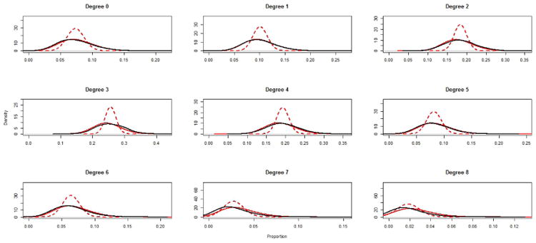
The black lines represent the target PPSNSD. The solid red lines represent the simulated PPSNSD using the proposed methods; the red dashed lines represent the simulated degree distribution for the ERGM.
Using our proposed methods, the simulated joint distribution was constructed by generating networks with the PPND and PPSNSD defined in equations (33) and (32), respectively. 100,100,000 networks (100,000 removed for burn-in) were generated and every 1,000th network is used for analysis; the R package CCMnet used to generate these networks relies heavily on the code in the R package ergm (Handcock et al., 2012). The marginal plots in figure 1 is calculated by computing the degree distribution for each of the 100,000 simulated networks. The solid red lines represent the simulated PPSNSD. The solid red line in the first plot of figure 1 represents the proportion of nodes in all 100,000 simulated networks with degree 0. The remaining plots 2-9 of figure 1, represent the density of the proportion of nodes in all 100,000 simulated networks with degrees 1-8, respectively.
The joint distribution for the ERGM was based on a model with a parameter for each degree between 0 and 8. The coefficients for the 9 ERGM parameters were fit using the mean values from the Dirichlet-multinomial distribution in equation (32) restricted to valid degree distributions. The marginal distribution of the degree distribution for the ERGM is depicted in figure 1 as dashed red lines. The distribution is based on generating 100,100,000 networks (100,000 removed for burn-in) and using every 1,000th network for analysis. The ERGM was fit and simulated using the R package ergm (Handcock et al., 2012).
Figure 1 demonstrates the closeness of simulated PPSNSD using the proposed methods to the target PPSNSD, defined in equation (32) across all of the degrees between 0 and 8. Although the method described in this paper matches the targeted distribution closely, care still needs to be used when interpreting the collection of networks that are generated using this method. The PPND applies to the congruence classes, and not all vectors Ỹ are valid degree distributions, i.e. there exists at least one valid network, G, such that η(G) = Ỹ. Even with this caveat, figure 1 provides clear evidence of attainment of our goal: the close match between the simulated PPND and the PPND defined in equation (33).
The mean marginal values of the degree distribution simulated from the ERGM match the mean values of the target PPSNSD closely, but the distributions are quite different– the joint distribution associated with the ERGM is the distribution which maximizes the entropy. Although the purpose of the ERGM, typically to provide inference on the generative network process, and the methods proposed in this paper, sampling of networks, are different, it may be useful to compare the results of simulated networks from an ERGM to networks generated from the proposed method. The simulated networks drawn from the ERGM are based on an ERGM where the parameter estimates are derived from a maximum likelihood framework, and therefore only the mean values of the sufficient network statistics are necessary to fit the ERGM. Since the number of samples used to estimate the mean values are never considered when estimating or simulating from the ERGM, the simulated networks from the ERGM do not take into account the uncertainty in these mean estimates; therefore, the simulated networks may not accurately reflect the true underlying of uncertainty. The simple random sample design in this example easily yields unbiased estimates of the sufficient network statistics for the whole network. If additional complexity exists in the sampling designs, advanced methods, such as methods proposed in Handcock & Gile (2010) or Pattison et al. (2013), may be necessary to properly estimate ERGM parameters. Recently there has been development of methods to estimate parameters of an ERGM using Bayesian inference (Caimo & Friel, 2011); this approach allows for uncertainty about model parameters. Koskinen et al. (2013) extended the Bayesian inference methods to apply to partially observed network data. Our method could complement these advances; by specifying the PPSNSD based on the posterior distribution of ERGM parameters, networks can be generated consistent with the Bayesian estimates of ERGM parameters.
6 Data Analysis
This section focuses on sampling realizations of networks on a new population using data collected on multiple networks. In this setting, the uncertainty in sufficient network statistics arises from the variation in network properties across the multiple networks that have been observed. Methods for this setting may be very useful in predicting the effect of an intervention on a new community after data has been collected on such effects in similar communities.
6.1 Add Health Data
To demonstrate how the network generation methods can be used to sample realizations from the PPND in the setting wherein multiple networks have been observed, we make use of data from the National Longitudinal Study of Adolescent Health (Add Health). Add Health is a longitudinal study of a nationally representative sample of adolescents in grades 7-12 in the United States during the 1994-95 school year (Harris & Udry, 2012).
The data arose from a two-stage cluster design: the first stage developed a stratified, random sample of all high schools in the United States, and the second sampled a set of students from each school. The student's friendship networks were developed from a questionnaire in which students were asked to name at most five male and five female friends. To ensure results can be reproduced by all interested researchers, we use only the freely available public data despite some limitations.2 The free ADD Health dataset contains information from only a subset of students and schools available in the full dataset and the only available mixing pattern is the proportion of mixing between genders. In the analysis presented below, we ignore the fact that the data for each school is a subsample, and assume that the dataset represents the complete information for the school; the previous section considered subsampled networks. Therefore, the analytical tools are appropriate for researchers with the full ADD Health dataset, but the results are reproducible by everyone.
The free ADD Health dataset provides the number of total friendships stated by each individual and the proportion of those friendships that are between males and females. The directed edges in the Health network data were converted to undirected edges by assuming the existence of a friendship if either student named the other as a friend. The data for each school s ∈ {1, …, J} used in the analysis include the degree distribution (number of friendships) for each gender, Dmale (s) and Dfemale (s), and the proportion of mixing between genders, MM(s).
The ADD Health data permits investigation of the proposed methods in the setting where it is of interest to generate a ‘typical’ student friendship network based on the degree distribution for each gender and the proportion of mixing between the genders. As the degree distributions and the proportions of mixing between genders from the observed schools vary, there is no single degree distribution that characterizes a ‘typical’ school. However, some degree distributions are more plausible than others; for example, a school with no friendships, D = (1,0,0, … ,0), would be highly unusual. Therefore, probabilities are assigned to possible degree distributions for males and females and the proportion of mixing between genders based on the observed schools.
To develop a probability distribution on student friendship networks the Bayesian framework described in section 4 was used. The data from each of school consists of a vector containing the proportion of males with number of friends ranging from 0-32, the proportion of females with number of friends ranging from 0-32, and the proportion of friendships between males and females.
6.2 Bayesian Model
This section develops a model for the posterior predictive distribution, P(G̃|{G1, …,GJ}), where J is the total number of observed schools. In this example it is of interest to model the degree distribution for male and females, along with the proportion of friendships between males and females. Let Y = {Y1, …, YJ}, where Yi is the sufficient network statistics for school i, be the observed sufficient network statistics.
By using equation (28), the PPND can be expressed as the following,
| (34) |
To evaluate the PPSNSD only the values of the sufficient network statistics are necessary. Therefore, the PPND can be rewritten as the following:
| (35) |
where P(Ỹ|Y1, …, YJ) is the PPSNSD for the sufficient network statistics that include the degree distributions for males and females and the proportion of relationship between genders. For the data analysis in this paper, two multivariate normal likelihoods are used to model the proportions of numbers of friendships that take on values between 0 and 32 (maximum number of friendships observed in any school) for males and for females; a normal likelihood is also used to model the proportion of relationships between males and females. Therefore, the model needs to fit the joint distribution for 67 parameters (33 male degrees, 33 female degrees, and 1 mixing parameter between the genders). The likelihood for our Bayesian model is the following:
| (36) |
where
Let (μM, ΣM) and (μF, ΣF) denote the mean and covariance matrix for the degree distributions corresponding to males and females, respectively, while (μMF, ) denotes the mean and variance for the proportion of relationships between males and females. The priors for our Bayesian model are the following:
where NIW and NIG denote the normal-inverse-Wishart and normal-inverse-gamma distribution. Therefore the PPSNSD for the above model is the following,
| (37) |
where the expressions for the parameters of the two multivariate Student t distributions and the univariate Student t distribution can be found in Murphy (2007). By substituting the probability distribution defined by equation (37) into equation (35) the PPND can be written as the following,
| (38) |
Since equation (38) is defined for networks g ∈
, it is sufficient to define the PPSNSD only on network statistics associated with valid congruence class. However, for many network statistics it is not computationally feasible to identify all valid congruence classes, as is the case in this example; therefore, it is often easier to define a probability distribution for Ỹ, e.g. the PPSNSD, that has support over a larger domain; the PPSNSD defined in equation (37) has support over ℛ67. The proposed methods induce a probability distribution for Ỹ associated with valid congruence classes that maintains the probability ratios, i.e. the values of P(Ỹ0|Y, μ0, γ0, Σ0, V0, μ1, γ1 , α1, β1)/P(Ỹ1|Y, μ0, γ0, Σ0, V0, μ1, γ1, α1, β1) for valid network statistics Y0 and Y1, defined by the PPSNSD. Though the induced probability distribution on valid congruence classes provides a convenient approach to assigning a probability distribution by maintaining the relative ratios, caution is necessary as it is possible for the probability distribution restricted to valid congruence classes to have different characteristics compared to the PPSNSD.
6.3 Results
We illustrate our method by sampling networks consisting of 500 females and 500 males based on equation (38). Figures 2 and 3 depict the 95% prediction intervals (PIs) for the marginal distribution for each value of the degree distribution from 0-32 for females and males, respectively. The red and blue bars in figure 2 represent the target PPSNSD and the simulated PPSNSD for males, respectively. The open circle on each bar denotes the mean value of the marginal distribution. Figure 3 shows similar information as figure 2 but for females. Figure 4 depicts the marginal distribution regarding proportion of friendships between the genders for the target PPSNSD and the simulated networks.
Fig. 2.
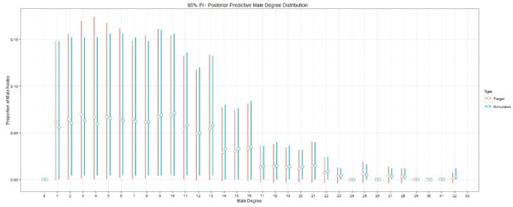
The red and blue bars represent the target PPSNSD and the simulated PPSNSD for males, respectively. The open circle on each bar denotes the mean value of the marginal distribution.
Fig. 3.
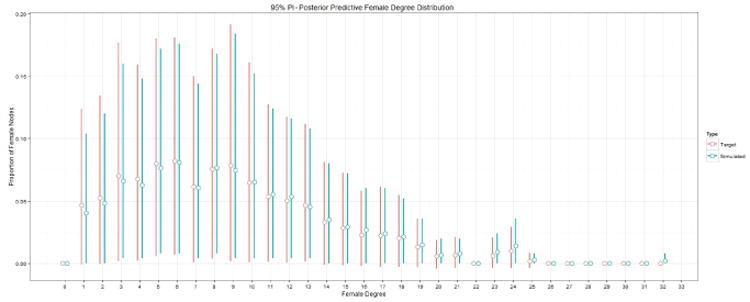
The red and blue bars represent the target PPSNSD and the simulated PPSNSD for females, respectively. The open circle on each bar denotes the mean value of the marginal distribution.
Fig. 4.
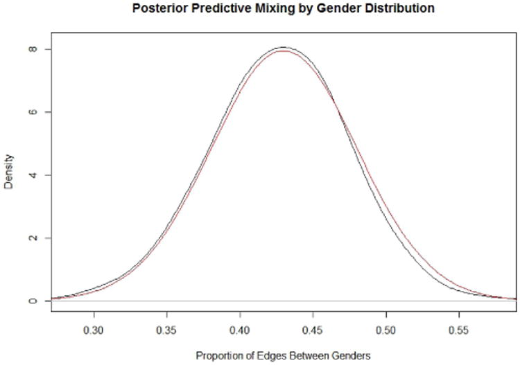
The marginal distribution regarding proportion of friendships between the genders for the target PPSNSD and the simulated networks.
The 95% PIs for the simulated networks are calculated by generating 500,500,000 networks (500,000 removed for burn-in) and then sampling every 1,000th network to use for analysis; the R package CCMnet used to generate these networks relies heavily on the code in the R package ergm (Handcock et al., 2012). The degree distribution for each of the 500,000 simulated networks is computed to calculate the 95% PIs. The target PPSNSD represented by equation (38) is equation (37) conditioned on Ỹ having a valid network realization. Because it is challenging to verify which Ỹ are valid, we approximate the target PPSNSD by looking at only the Ỹ for which all values are greater than -.005, as Ỹ must be positive, and the sum of Ỹ to be between .995 and 1.005.
In figures 2 and 3, the mean values for the target PPSNSD and the simulated PPSNSD are very close as are the 95% PIs. Figure 4 demonstrates that the entire marginal PPSNSD with regards to mixing between genders for the target distribution and for simulated networks are very close. These results show that the methods proposed in this paper can be used to model a complex PPND with a large number of sufficient network statistics.
The PPSNSD represented by equation (38) and depicted in figures 2 and 3 shows wide prediction intervals in the marginal distributions for many degrees for both males and females. The width of the intervals provides evidence of large heterogeneity in the friendship networks across schools; methods for network sampling must capture the heterogeneity in friendships networks to make possible realistic simulations of school-based interventions, such as smoking prevention programs. The PPSNSD can be made more flexible, for example by incorporating the between-gender degree distribution correlation; but with 67 parameters already in the model applied to only 132 schools, some simplifying assumptions are necessary in this example. Incorporating a between-gender correlation structure might result in greater correlation in width of prediction intervals between genders, we do not think it likely that doing so would result in much more narrow intervals. To generate networks that characterize only a subset of schools to simulate interventions geared to such schools, specifying the PPSNSD by a regression model that controls for school-wide covariates may narrow the prediction intervals. Regardless of whether interest lies in generating networks representing specific types of schools or all of those in the sample, the methods presented in this paper can accommodate different levels of heterogeneity across networks.
7 Discussion
This paper presents novel methods to incorporate uncertainty in values of sufficient network statistics in the generation of networks. The network properties of density, degree distribution, mixing patterns and clustering are used to illustrate the approach. These network properties have been shown to have great influence on processes operating on diverse areas such as Internet connectivity, biological interactions, and spread of sexually transmitted infections (STIs).
The proposed methods allow generation of collections of networks based on a user-defined posterior predictive sufficient network statistic distribution. The examples in sections 5 and 6 used reasonably flexible models for the PPSNSD. However, the nature of social networks are complex; and it may be useful to take additional network properties into account, such as degree assortativity and interactions between the male and female degree distributions. The examples modeled the uncertainty that arises from sampling; but the methods can also be used to incorporate uncertainty that results from errors in self-reported data, information about which may be developed from inconsistencies in these data. The proposed methods are well suited for modeling and analyzing data involving two large cluster randomized controlled trials (CRCTs) supported by the US President's Emergency Plan for AIDS Relief to study the impact of combination prevention packages on HIV incidence (Wang et al., in press; Boily et al., 2012). Both CRCTs plan to collect information on network properties that includes degree distribution (number of sexual partners) and demographics mixing patterns. The goal of the studies includes not only measurement of the efficacy of the intervention, but also provision of information that informs the development of realistic models used to predict the potential benefits of the interventions in communities elsewhere in Sub-Saharan Africa. One way to construct such models is through simulation of epidemic processes on collections of contact networks. As it is unfeasible to collect detailed data from new communities where the interventions may be deployed, it will be useful to generate network collections that reflect plausible ranges of network properties for such communities. This collection must not only capture the variation in network property values across the observed study communities, but also permit investigation of the sensitivity of model-based predictions to assumptions regarding these new communities. These assumptions must reflect uncertainty in network properties that arises both in the characterization of networks that have been studied, and in the degree to which networks in new communities may differ from the observed networks. For example, the prior distribution of network properties may be made more diffuse to reflect uncertainty about the comparability of networks that have been studied and those that have not.
The ability to accommodate uncertainty in estimated network properties in the generation of collections of networks allows investigators to assess the level of precision in these estimates that is needed for reliable evaluation of the relative merits of different policy options. Hence, these approaches can be useful in designing randomized trials of community-level control strategies in settings where infections or behaviors diffuse over social or sexual networks.
Further research is needed to expand this framework to include additional network properties. Though the methods allow for great flexibility in specifying the PPSNSD, there are limitations on the types of sufficient network statistics that can be accommodated. For each sufficient network statistic one must be able to derive an expression for the ratio f(Cgpt+1,Cgt)/f(Cgt, Cgpt+1) in equation (4). There may exist a general formulation of the ratio for all or some sufficient network statistics, however none is currently known. In section 3, we derive expressions for common sufficient network statistics, including the ones most applicable to disease modeling. Further research is necessary to investigate the impact of the degree of accuracy of approximations for network properties on performance of our methods, in a variety of settings such as those with small network sizes.
A promising area of further research is to use this framework in generating dynamic networks. In many complex systems the variation of network properties over time may be difficult measure, and therefore, need flexible models to handle uncertainty.
Supplementary Material
Acknowledgments
We would like to thank Ted Cohen for his useful comments. This research is supported by grants from the National Institute of Health (T32NS048005, R37 AI-51164).
Footnotes
R package CCMnet is currently available by request.
The authors would be glad to provide instructions and code to download and format the data to replicate results
Conflict of Interest: None declared.
Contributor Information
Ravi Goyal, Email: rgoyal@hsph.harvard.edu, Department of Biostatistics, Harvard School of Public Health.
Victor De Gruttola, Department of Biostatistics, Harvard School of Public Health.
Joseph Blitzstein, Department of Statistics, Harvard University.
Bibliography
- Amanatidis Yorgos, Green Bradley, Mihail Milena. Graphic realizations of joint-degree matrices. Unpublished 2008 [Google Scholar]
- Bansal S, Pourbohloul B, Meyers LA. A comparative analysis of influenza vaccination programs. Plos medicine. 2006;3:387. doi: 10.1371/journal.pmed.0030387. [DOI] [PMC free article] [PubMed] [Google Scholar]
- Barabasi Albert-Laszlo, Albert Reka. Emergence of scaling in random networks. Science. 1999;286:509–512. doi: 10.1126/science.286.5439.509. [DOI] [PubMed] [Google Scholar]
- Blitzstein Joseph, Diaconis Persi. A sequential importance sampling algorithm for generating random graphs with prescribed degrees. Internet mathematics. 2010;6(4):487–520. [Google Scholar]
- Boily Marie-Claude, Mâsse B, Alsallaq R, Padian N, Eaton J, Vesga J, Hallett T. Hiv treatment as prevention: Considerations in the design, conduct, and analysis of cluster randomized controlled trials of combination hiv prevention. Plos med. 2012;9(7):e1001250. doi: 10.1371/journal.pmed.1001250. [DOI] [PMC free article] [PubMed] [Google Scholar]
- Bollobás Béla. Random graphs. 2. New York: Cambridge University Press; 2001. [Google Scholar]
- Britton Tom, Deijfen Maria, Martin-Lo¨f Anders. Generating simple random graphs with prescribed degree distribution. Journal of statistical physics. 2006;124(6):1377–1397. [Google Scholar]
- Caimo Alberto, Friel Nial. Bayesian inference for exponential random graph models. Social networks. 2011;33(1):41–55. [Google Scholar]
- Christakis Nicholas, Fowler James. The collective dynamics of smoking in a large social network. New england journal of medicine. 2008;358(21):2249–2258. doi: 10.1056/NEJMsa0706154. [DOI] [PMC free article] [PubMed] [Google Scholar]
- Doyle John C, Alderson David, Li Lun, Low Steven, Roughan Matthew, Shalunov Stanislav, Tanaka Reiko, Willinger Walter. The ‘robust yet fragile’ nature of the internet. Proceedings of the national academy of sciences. 2005;102(41):14497–14502. doi: 10.1073/pnas.0501426102. [DOI] [PMC free article] [PubMed] [Google Scholar]
- Dunbar RIM. Coevolution of neocortical size, group size, and language in humans. Behavioural and brain sciences. 1993;16:681–735. [Google Scholar]
- Erdős Paul, Rényi Albért. On the evolution of random graphs. Publications of the mathematical institute of the hungarian academy of sciences. 1960;5:17–61. [Google Scholar]
- Frank O. Network sampling and model fitting. In: Carrington PJ, Scott J, Wasserman S, editors. Models and methods in social network analysis. Chap. 3. Cambridge: Cambridge Univ. Press; 2005. pp. 31–56. of: [Google Scholar]
- Frank Ove, Strauss David. Markov graphs. Journal of the american statistical association. 1986;81:832–842. [Google Scholar]
- Friedgut Ehud, Kalai Gil. Every monotone graph property has a sharp threshold. Proceedings of the american mathematical society. 1996;124(10) [Google Scholar]
- Hakimi SL. On realizability of a set of integers as degrees of the vertices of alinear graph. Journal of the society for industrial and applied mathematics. 1962;10:496–506. [Google Scholar]
- Handcock Mark S. Version 1.2. Seattle, WA: 2003. degreenet: Models for skewed count distributions relevant to networks. Project home page at http://statnet.org. [Google Scholar]
- Handcock Mark S, Gile Krita J. Modeling social networks from sampled data. Annals of applied statistics. 2010;4:5–25. doi: 10.1214/08-AOAS221. [DOI] [PMC free article] [PubMed] [Google Scholar]
- Handcock Mark S, Hunter David R, Butts Carter T, Goodreau Steven M, Krivitsky Pavel N, Morris Martina. Version 3.0-1. Seattle, WA: 2012. ergm: A package to fit, simulate and diagnose exponential-family models for networks. Project home page at urlstatnet.org. [DOI] [PMC free article] [PubMed] [Google Scholar]
- Harris Kathleen Mullan, Udry J Richard. National longitudinal study of adolescent health (add health), 1994-2008. Ann Arbor, MI: Inter-university Consortium for Political and Social Research; 2012. 10.3886/icpsr21600-v9 edn. [Google Scholar]
- Havel V. A remark on the existence of finite graphs. Časopis pest mat. 1955;80:477–480. [Google Scholar]
- Kolaczyk E. Chap Sampling and Estimation in Network Graphs. New York: Springer Science+Business Media, LLC; 2009. Statistical analysis of network data: Methods and models; pp. 123–152. [Google Scholar]
- Koskinen Johan H, Robins Garry L, Wang Peng, Pattison Philippa E. Bayesian analysis for partially observed network data, missing ties, attributes and actors. Social networks. 2013;35(4):514–527. [Google Scholar]
- Mahadevan P, Krioukov D, Fall K, Vahdat A. Systematic topology analysis and generation using degree correlations. Proceedings of the acm sigcomm 2006 [Google Scholar]
- Maslov Sergei, Sneppen Kim. Specificiy and stability in topology of protein networks. Science. 2002;296(5569):910–913. doi: 10.1126/science.1065103. [DOI] [PubMed] [Google Scholar]
- McNeely Clea A, Nonnemaker James M, Blum Robert W. Promoting school connectedness: Evidence from the national longitudinal study of adolescent health. Journal of school health. 2002;72:138–146. doi: 10.1111/j.1746-1561.2002.tb06533.x. [DOI] [PubMed] [Google Scholar]
- McPherson Miller, Smith-Lovin Lynn, Brashears Matthew E. Social isolation in america: Changes in core discussion networks over two decades. Americansociological review. 2006;71(3):353–375. [Google Scholar]
- Meyers LA, Newman MEJ, Martin M, Schrag S. Applying network theory to epidemics: Control measures for mycoplasma pneumoniae outbreaks. Emerging infectious diseases. 2003;9(2):204. doi: 10.3201/eid0902.020188. [DOI] [PMC free article] [PubMed] [Google Scholar]
- Meyers Lauren Ancel, Pourbohloul Babak, Newman Mark EJ, Skowronski Danuta M, Brunham Robert C. Network theory and sars: predicting outbreak diversity. Journal of theoretical biology. 2005;232(1):71–81. doi: 10.1016/j.jtbi.2004.07.026. [DOI] [PMC free article] [PubMed] [Google Scholar]
- Mills Harriet L, Cohen Theodore, Colijn Caroline. Modelling the performance of isoniazid preventive therapy for reducing tuberculosis in hiv endemic settings: the effects of network structure. Journal of the royal society interface. 2011;8(63):1510–1520. doi: 10.1098/rsif.2011.0160. [DOI] [PMC free article] [PubMed] [Google Scholar]
- Morris M, Kurth A, Hamilton D, Moody J, Wakefield S. Concurrent partnerships and hiv prevalence disparities by race: Linking science and public health practice. American journal of public health. 2009;99(6):1023–1031. doi: 10.2105/AJPH.2008.147835. [DOI] [PMC free article] [PubMed] [Google Scholar]
- Morris Martina, Goodreau Steven, Moody James. Sexual networks, concurrency, and std/hiv. In: Holmes KK, Sparling PF, Stamm WE, editors. Sexually transmitted diseases. New York, NY, USA: McGraw-Hill International Book Co; 2007. pp. 109–126. of: [Google Scholar]
- Murphy Kevin P. Conjugate bayesian analysis of the gaussian distribution 2007 [Google Scholar]
- Newman Mark. Assortative mixing in networks. Physical review letters. 2002;89(20):208701. doi: 10.1103/PhysRevLett.89.208701. [DOI] [PubMed] [Google Scholar]
- Newman Mark E. Networks an introduction. New York: Oxford University Press; 2010. [Google Scholar]
- Palombi Leonardo, Bernava Giuseppe M, Nucita Andrea, Giglio Pietro, Liotta Giuseppe, Nielsen-Saines Karin, Orlando Stefano, Mancinelli Sandro, Buonomo Ersilia, Scarcella Paola, Altan Anna Maria Doro, Guidotti Gianni, Ceffa Susanna, Haswell Jere, Zimba Ines, Magid Nurja Abdul, Marazzi Maria Cristina. Predicting trends in hiv-1 sexual transmission in sub-saharan africa through the drug resource enhancement against aids and malnutrition model: Antiretrovirals for reduction of population infectivity, incidence and prevalence at the district level. Clinical infectious diseases. 2012 doi: 10.1093/cid/cis380. [DOI] [PubMed] [Google Scholar]
- Pattison Philippa E, Robins Garry L, Snijders Tom AB, Wang Peng. Conditional estimation of exponential random graph models from snowball sampling designs. Journal of mathematical psychology 2013 [Google Scholar]
- Robert Christian P, Casella George. Monte carlo statistical methods. New York: Springer; 2004. [Google Scholar]
- Shalizi Cosma Rohilla, Rinaldo Alessandro. Consistency under sampling of exponential random graph models. Annals of statistics. 2013;41(2):508–535. doi: 10.1214/12-AOS1044. [DOI] [PMC free article] [PubMed] [Google Scholar]
- Valente Thomas W. Network interventions. Science. 2012;337:49–53. doi: 10.1126/science.1217330. [DOI] [PubMed] [Google Scholar]
- Valente Thomas W, Hoffman Beth R, Ritt-Olson Annamara, Lichtman Kara, Johnson C Anderson. Effects of a social-network method for group assignment strategies on peer-led tobacco prevention programs in schools. American journal of public health. 2003;93(11):1837–1843. doi: 10.2105/ajph.93.11.1837. [DOI] [PMC free article] [PubMed] [Google Scholar]
- V´zquez Alexei, Pastor-Satorras Romualdo, Vespignani Alessandro. Large-scale topological and dynamical properties of the internet. Physical review e. 2002;65(6):66130. doi: 10.1103/PhysRevE.65.066130. [DOI] [PubMed] [Google Scholar]
- Wang Rui, Goyal Ravi, Lei Quanhong, Essex Max, DeGruttola Victor. Sample size considerations in the design of cluster randomized trials of combination hiv prevention. Clinical trials. doi: 10.1177/1740774514523351. in press. [DOI] [PMC free article] [PubMed] [Google Scholar]
- Watts Duncan J, Strogatz Steven H. Collective dynamics of ‘small-world’ networks. Internet mathematics. 1998;393(6684):397–498. doi: 10.1038/30918. [DOI] [PubMed] [Google Scholar]
Associated Data
This section collects any data citations, data availability statements, or supplementary materials included in this article.