Functional Data Analysis of Tree Data Objects

Abstract

Data analysis on non-Euclidean spaces, such as tree spaces, can be challenging. The main contribution of this paper is establishment of a connection between tree data spaces and the well developed area of Functional Data Analysis (FDA), where the data objects are curves. This connection comes through two tree representation approaches, the Dyck path representation and the branch length representation. These representations of trees in Euclidean spaces enable us to exploit the power of FDA to explore statistical properties of tree data objects. A major challenge in the analysis is the sparsity of tree branches in a sample of trees. We overcome this issue by using a tree pruning technique that focuses the analysis on important underlying population structures. This method parallels scale-space analysis in the sense that it reveals statistical properties of tree structured data over a range of scales. The effectiveness of these new approaches is demonstrated by some novel results obtained in the analysis of brain artery trees. The scale space analysis reveals a deeper relationship between structure and age. These methods are the first to find a statistically significant gender difference.

1 Introduction

Functional data analysis (FDA) offers many powerful statistical tools for analyzing a population of curves, and its methodology and application has been well documented in Ramsay and Silverman (2002, 2005) and Ferraty and Vieu (2006). Wang and Marron (2007) extended the realm of FDA to the domain of Object Oriented Data Analysis (OODA). In OODA, the atoms of the analysis are more general data objects, such as shapes, which naturally lie in smooth manifolds, and tree structured data that lie in strongly non-Euclidean spaces (in the sense that there is no approximating tangent planes). A major contribution of Wang and Marron (2007) was the development of an analog of principal component analysis (PCA) (Jolliffe, 2002) for tree data objects, which extended this central methodology of FDA from standard Euclidean spaces to non-Euclidean tree spaces. This work has generated substantial research in the OODA of tree structured data objects, see Aydin et al. (2009); Aydin et al. (2011, 2012).

The current paper focuses on new analytical tools for the analysis of tree-structured data. The challenge of tree data is that fundamental Euclidean concepts that underlie conventional FDA, such as linear subspace, projection, linear combination, and thus PCA, are not available in a straightforward way. The above referenced works dealt with this problem by developing analogs of PCA for tree spaces. Here we take a much different approach, motivated by an important connection, from probability theory, between random trees and standard stochastic processes. In particular, we use the Dyck path representation (DPR) (Harris, 1952). This was invented in the stochastic process literature as a tool for asymptotic analysis of branching processes. This represents trees as curves, so the rich suite of FDA tools that have already been developed can be readily exploited to analyze populations of tree structured data objects. Our approach offers a valuable alternative for analyzing tree data, and bypasses the often challenging optimization problems that lie at the heart of the earlier works.

Our main contributions are as follows. We first formally introduce the DPR. Careful thought about DPR led us to a second, parallel approach called branch length representation (BLR). Correspondence between trees is derived using the concept of support tree, which contains the topological structure of the union of the individual trees. The support tree concept enables FDA to be performed on the transformed collection of trees in the corresponding curve space. Furthermore, in order to analyze the tree-structure variation in a scale-space fashion, we introduce the idea of tree pruning and define the corresponding concepts of pruned support tree and individual pruned tree. The scale-space approach allows us to fine tune the tree analysis at a range of scales.

There are a variety of other methods that have been used to analyze tree data. Billera et al. (2001) presented several methods to analyze phylogenetic trees. A drawback to such an approach for the brain artery data is that it requires a common leaf set. Shawe-Taylor and Cristianini (2004) introduced a number of kernel-based algorithms for analyzing tree-structured data. Collins and Duffy (2001) applied tree kernels to study language tree problems. Tree kernel-based methods were used by Eom et al. (2006) to study protein-protein interaction mining in the biomedical literature, and by Yamanishi et al. (2007) and Vert (2002) to classify the glycan tree and phylogenetic profiles respectively in bioin-formatics.

The remainder of the paper is organized as follows. In Section 2 we describe the brain artery tree data (Aylward and Bullitt, 2002) that motivated our research. Section 2.1 presents the notion of descendant correspondence to embed the 3-dimensional brain artery trees into 2 dimensions. Section 3 introduces two tree representation methods: DPR and BLR in Sections 3.2 and 3.3, respectively. Section 4 presents the DPR analysis of individual trees. Section 4.4 presents the BLR analysis of individual trees. Section 5 introduces the idea of tree pruning, and extends the DPR and BLR analyses to individual pruned trees under a range of pruning levels, which offers a more detailed scale-space analysis of tree data objects. In particular, the tree pruning idea is used to study the relationship of age (gender) with some summaries of the trees, including total branch length (TBL), average branch length (ABL), and the number of non-missing branches (NNB) of each individual pruned tree. Among other things, the analysis revealed that the age relationship with TBL changes from being negative to positive for individual pruned trees, as the pruning level increases; this interesting phenomenon can be explained neurologically, and was further confirmed through a multiple comparison adjustment that accounts for the scale-space framework. In addition, we were able to find, for the first time, that the NNB is significantly different between males and females.

Our methodology could also be applied to other data sets, containing tree structured data objects. These include other natural vascular systems (e.g. retinal or breast), as well as other anatomical tree structures, such as lung airways, as discussed in Feragen et al. (2010). These ideas have the potential for use outside of medical imaging as well. With more work, they could be adapted to graph structured data objects, as in the active areas of social and computer networks.

2 Data Description

Our driving real data example is a set of human brain artery trees. This data set is from a study of Magnetic Resonance Angiography (MRA) brain images (Dumoulin and Hart, 1986) of a set of 98 human subjects. Long term goals are to study stroke and to find loci of pathologies such as brain tumors. However, in this study only carefully screened normal subjects are considered. To build methodology for studying the long term goals, we here focus on the available covariates of gender and age (from 19 to 79). The raw data can be found at Handle (2008). A detailed description of the data can be found in Section A of the supplementary material. In most analyses presented here, only the back tree, shown in gold in Panel (B) of Figure A of the supplementary material, will be shown explicitly, as that usually gave the most interesting results.

2.1 Correspondence

Statistical analysis is enhanced by representing the 3 dimensional brain trees, using an embedding in 2 dimensions. In general there are many ways to embed. Looking across the data set, it is desirable for similar branches to correspond in the embedding. This is a correspondence problem, similar to the one that has appeared in image and shape analysis, see e.g. Chapter 1 of Dryden and Mardia (1998). Aydin et al. (2009) provide several approaches to the embedding problem in the tree context.

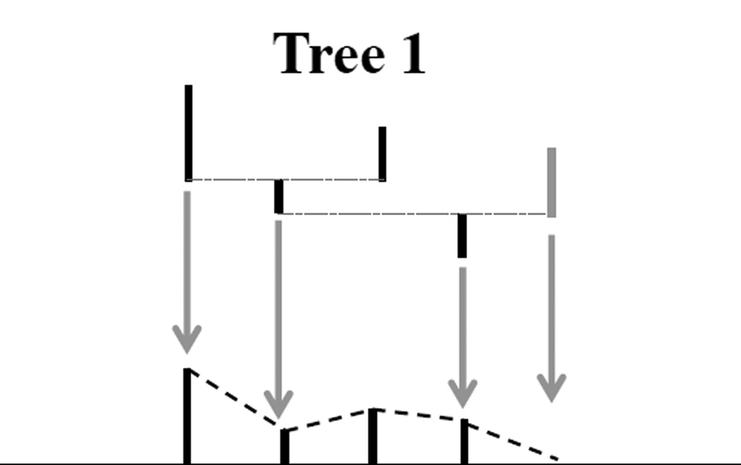
The descendant correspondence method in Aydin et al. (2009) is used here to embed the 3-dimensional tree as a binary tree. The goal of descendant correspondence is to orient the tree, so that at each vertex the left branch has more descendants than the right branch. Figure 1 illustrates how we attain descendant correspondence by flipping branches. By flipping the branches of Tree 1 on both sides of the vertex (highlighted by the gray arrow), Tree 1 becomes Tree 2. Similarly, we can flip the branches of Tree 2 on the highlighted vertex to generate Tree 3. Given an arbitrary tree, it can be put in descendant correspondence form by a series of flipping operations (an algorithmically useful concept). For example, the tree shown in Figure 2 is a transformed version of a brain artery tree using the descendant correspondence. A 3-d representation to the original artery structure can be found in Panel (B) of Figure A in the supplementary material. The tree represented in Figure 2 corresponds to that back (gold) subtree.

Figure 1.

Toy example illustrating Descendant Correspondence: Given Tree 1, two flipping operations put most descendant branches to the left, resulting in Tree 3.

Figure 2.

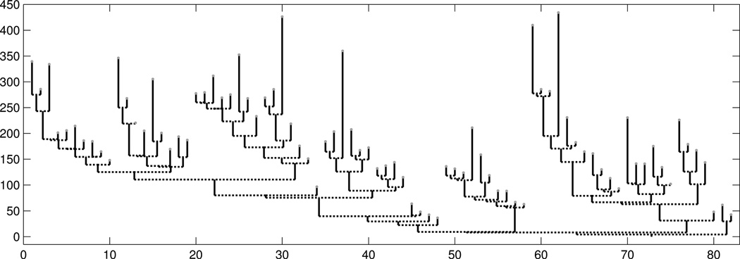
This tree is transformed from a real brain artery tree, using descendant correspondence. The lengths of the vertical line are the branch lengths. The horizontal axis shows the corresponding branch number.

We now use Figure 2 to introduce several key concepts related to this 2-d embedding of trees. As noted above, tree branches are vessel segments between two consecutive splitting points of the blood vessels. A leaf branch is the vessel segment between the end point of a blood vessel and its nearest splitting point. The arc length of each vessel segment, following the vessel curve (as shown in Panel (B) of Figure A of the supplementary material), is defined to be the branch length. Every non-leaf branch of the brain trees connects its children branches to its parent. The vertical line segments in Figure 2, and their lengths represent tree branches, and their respective branch lengths. The root branch at the bottom of Figure 2 corresponds to the initial trunk, as shown in Figure A of the supplementary material. The y-axis in Figure 2 is the arc distance from the root. The x-coordinate of each leaf branch is an integer value (1, ⋯ , m, the number of leaves). The leaves are ordered so there are no crossing branches, and the descendant correspondence holds. The x-coordinate of each connecting branch is the midpoint of the x-coordinates of the two branches that it connects. We will focus on tree structured data objects of this type and explore the population structure of 98 such objects.

3 Tree Representation

In this section we introduce two tree representation approaches to transform trees into Euclidean curves: the Dyck path representation (DPR) (Section 3.2) and the branch length representation (BLR) (Section 3.3). As noted above, each representation approach establishes a one-to-one correspondence between trees and a subset of curves, which allows use of the very wide range of FDA methods.

3.1 Support Tree

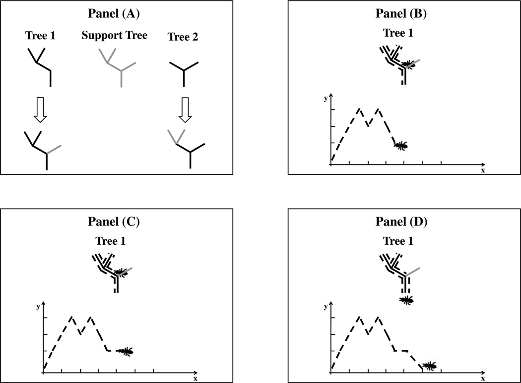
To keep corresponding parts of the trees aligned in the DPR and BLR, they are put into a structural context called the support tree. The support tree is essentially the union of the individual trees’ branches where the branch length information is deliberately neglected, while keeping their topological (i.e. connectivity) information. Panel (A) of Figure 3 illustrates how to define the support tree of a set of individual trees. Ignoring the branch length information of the individual trees (by setting them all to unit length), we take the union of these branches to construct the support tree. We set the branches of the support tree to have unit length. The support tree contains the total topological structure of the full set of individual trees.

Figure 3.

Construction of a Support Tree and Dyck Path Representation (DPR). Panel (A) shows in gray the support tree of trees 1 and 2: the union of the individual trees’ branches where branch length information is deliberately ignored. Panels (B) to (D) show construction of the Dyck path of an individual tree in the support tree context.

Next each individual tree is put into the support tree structure by keeping the original branches and considering the other branches of the support tree to be missing. This is illustrated in Panel (A) of Figure 3, where the mapping of Trees 1 and 2 into the support tree structure are indicated by the arrows. Note that the gray is used for the missing branches. In both the DPR and BLR, the length of these missing branches is considered to be zero. Panels (B)-(D) illustrate the moving ant representation of the DPR of Tree 1 under the support tree structure, which will be discussed in Section 3.2.

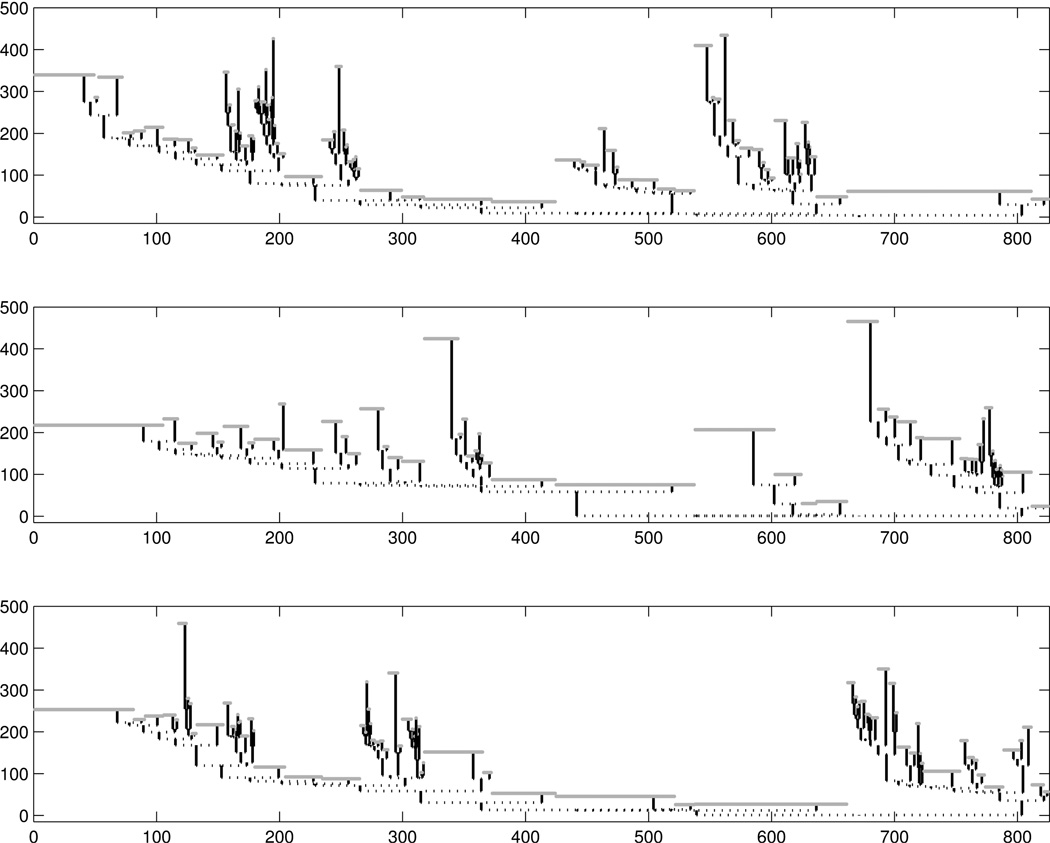
The top panel of Figure 4 shows the tree from Figure 2 under the support tree structure, relative to the population of 98 trees. The flat parts are support tree branches that are missing in this particular tree. Such branches are illustrated as gray branches in the lower part of Panel (A) in Figure 3. To give an indication of the variability in the population, two other back trees are shown in the remaining panels. Each tree has many missing branches under the support tree structure, and the positions of these missing branches are very different among the individual trees. This is a common feature of all 98 population trees.

Figure 4.

Three Individual Trees in the Support Tree Context. The top panel tree corresponds to the tree in Figure 2. The gray flat parts in these trees correspond to missing branches.

3.2 Dyck Path Representation in Support Tree Context

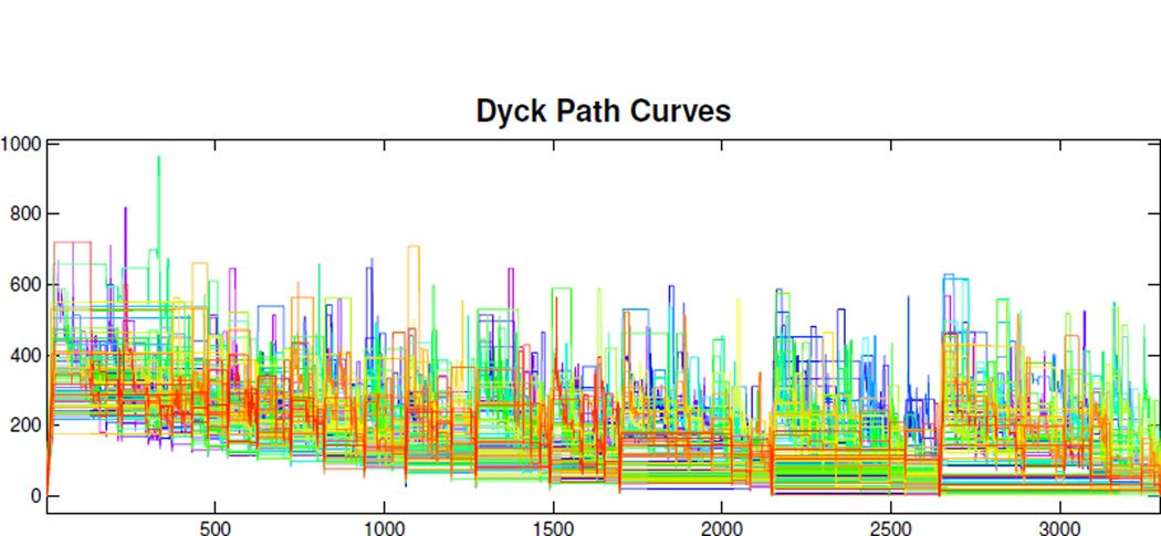
In stochastic process theory, there is a large literature studying asymptotics of random trees, such as branching processes, using a connection between trees and curves called the Dyck path representation (DPR). This provides a useful bridge between tree spaces and curve spaces, which makes a tree uniquely correspond to a curve. The DPR can be understood as follows. The toy example in Figure 3 illustrates this process. The DPR of Tree 1 is a dashed piecewise curve, connecting the coordinate points (x, y) where the x-coordinate tracks the number of time steps as the ant walks around Tree 1 and the y-coordinate is the corresponding branch distance to the root. Since the gray branch of Tree 1 is missing, as shown in Panel (A) of Figure 3, the segment of the DPR corresponding to that branch is a flat line as shown in Panels (C) and (D) of Figure 3. The collection of the DPR curves for all 98 binary (back) trees under the support tree structure is shown in Figure 5. The color of each DPR curve uses a rainbow color scheme to represent age, ranging from magenta (young, age 19) to red (old, age 79). Though the support tree structure depends on the individual trees, deleting or adding a sample tree will not dramatically change the support tree structure because of the descendant correspondence described in Section 2.1.

Figure 5.

The DPR Curves of Population Trees. The color ranges from magenta (for young) to red (for old).

It is worth noticing that, from the definition of DPR, every branch of the support tree is passed twice, so the same branch distance to the root appears twice in the DPR curves in Figure 5. The right endpoint of the x-coordinate range is twice the number of branches in the support tree. In addition, since there are many missing branches for the individual trees under the support tree structure context, as shown in Figure 4, there are many flat segments on the DPR curves, as shown in in Figure 5. Also, some individual binary trees have some extremely long branches, shown in Figure 4, suggesting that the DPR curves have jumps as shown in Figure 5. It follows from the descendant correspondence that the left part of the DPR curves in Figure 5 is generally higher than the right.

In Section 4 we will apply FDA methods to this family of curves. A very common FDA approach, see Ramsay and Silverman (2002, 2005), is to assume that the underlying data objects are smooth curves, together with substantial measurement noise, which is viewed as a nuisance. Good software for this approach to FDA includes PACE (Yao et al., 2003). For this Dyck Path data, we take a different approach, because our curves are clearly not smooth underlying signal plus noise. In particular, the essentially rectangular corners that are ubiquitous are not nuisance artifacts, but instead represent very important underlying tree structure. Smoothing them away would mean a loss of critical information, not a noise reduction.

3.3 Branch Length Representation in Support Tree Context

The branch length representation (BLR) is a modification of the DPR. Instead of recording branch distance to the root, as in DPR, BLR constructs pairs of coordinates (x, y), as shown in Figure 6. Each x-coordinate is the branch number from left to right in the order of their appearance in the descendant correspondence, defined in Section 2.1. Each y-coordinate is the length of the branch. These (x, y) pairs are piecewise linearly connected to form a curve as in Figure 6. The BLR records just the length of each branch that the ant passes at every step. Note that the BLR curve goes to 0 at each missing branch.

Figure 6.

Example of Construction of the Branch Length Representation (BLR) using Tree 1 from Figure 3. Each vertical branch is represented by a vertical line segment, whose base is at the corresponding point on the horizontal axis, and whose height is the branch length, with the length of missing (gray) branches set to 0. The piecewise line connecting the upper end (dashed) is the BLR.

Panel (A) in Figure 7 shows the BLR curves of the 98 population trees. The color corresponds to age, as in Figure 5. While it is difficult to distinguish individual curves in Panel (A) of Figure 7, each branch length curve has many y = 0 flat parts due to missing branches. One way to see this is to view the full size version of this plot in Figure B of the supplementary material. Another way to understand the many zeros in each curve is to view just one of these curves, as shown in Panel (B). This is chosen to have the median number of zeros, but maintains its age coloring from the full data set. This curve shows many flat parts and is very typical of the other BLR curves. The right endpoint of the x-coordinate range for the plots in Panels (A) and (B) of Figure 7 is 1649, the number of branches in the support tree. It is half of the right endpoint (3298) in the DPR curves in Panel (C) of Figure 7, because every branch is passed twice in the DPR curves. The y-coordinate is the branch length in these curves, in contrast to the branch height (measured from the root, i.e. cumulative height) shown in Panel (C). It follows that the top of the y-coordinate range is much smaller in Panels (A) and (B) than in Panel (C).

Figure 7.

Panel (A) shows the BLR representation of the full data set. The color again ranges from magenta (for young) to red (for old). Panel (B) shows just one of the curves in the left panel, using a thicker line width. Panel (C) is the DPR representation of the full data set, same as in Figure 5.

4 Dyck Path Analysis

Now we can use FDA techniques on this sample of DPR curves to study variation in the population, as well as relationships with gender and age.

4.1 Principal Component Analysis

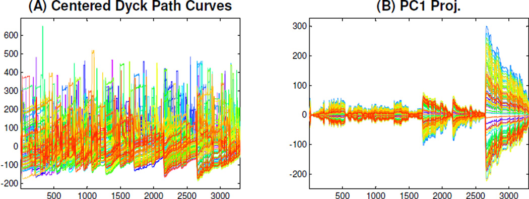
In this section, we perform PCA on these DPR curves, as shown in Figure 8. Consider each curve in Figure 5 as a d-dimensional vector X_i, i = 1, ⋯ ,n (n = 98 is the number of DPR curves). Subtracting the mean X̅ from each X_i gives the centered curve X_i − X̅, shown in Panel (A) of Figure 8. A full size version of the centered curves are in Figure C of the supplementary material. Denote the d × n centered DPR data matrix as X = [X₁ − X̅, ⋯, X_n − X̅], and then the matrix $X/\sqrt{n-1}$ has the following singular value decomposition, see discussions in Section 3 of Shen et al. (2012):

$$X/\sqrt{n-1}=\sum _{k=1}^r{d}_k{u}_k{v}_k^T,$$

where r is the rank of X, which is less than or equal to min(d, n). In addition, d₁ ≥ ⋯ ≥ d_r ≥ 0 are singular values, u_k is the kth PC direction, d_kv_k is the kth PC score vector. Write the k-th PC score vector d_kv_k in the form

$$d_k{v}_k={(s_{1,k},\cdots ,s_{n,k})}^T,k=1,\cdots ,r.$$ (2)

Figure 8.

PCA of the DPR Curves. The DPR curves are first mean centered, Panel (A), and then projected onto the first PC direction, Panel (B), to explore the modes of the variation of the DPR curves. Panel (B) shows most of this dominant mode of variation occurs on the right side.

Useful visualization comes from the PC1 projected curves s_i,1u₁ (shown in Panel (B) of Figure 8). These show that most of this dominant component of variation is on the right side. This suggests that variation in the right part of the trees drives this component. We further explore this mode of variation in Figure 9. The projections of these curves onto the second and third PC directions appear in Figure D of the supplementary material.

Figure 9.

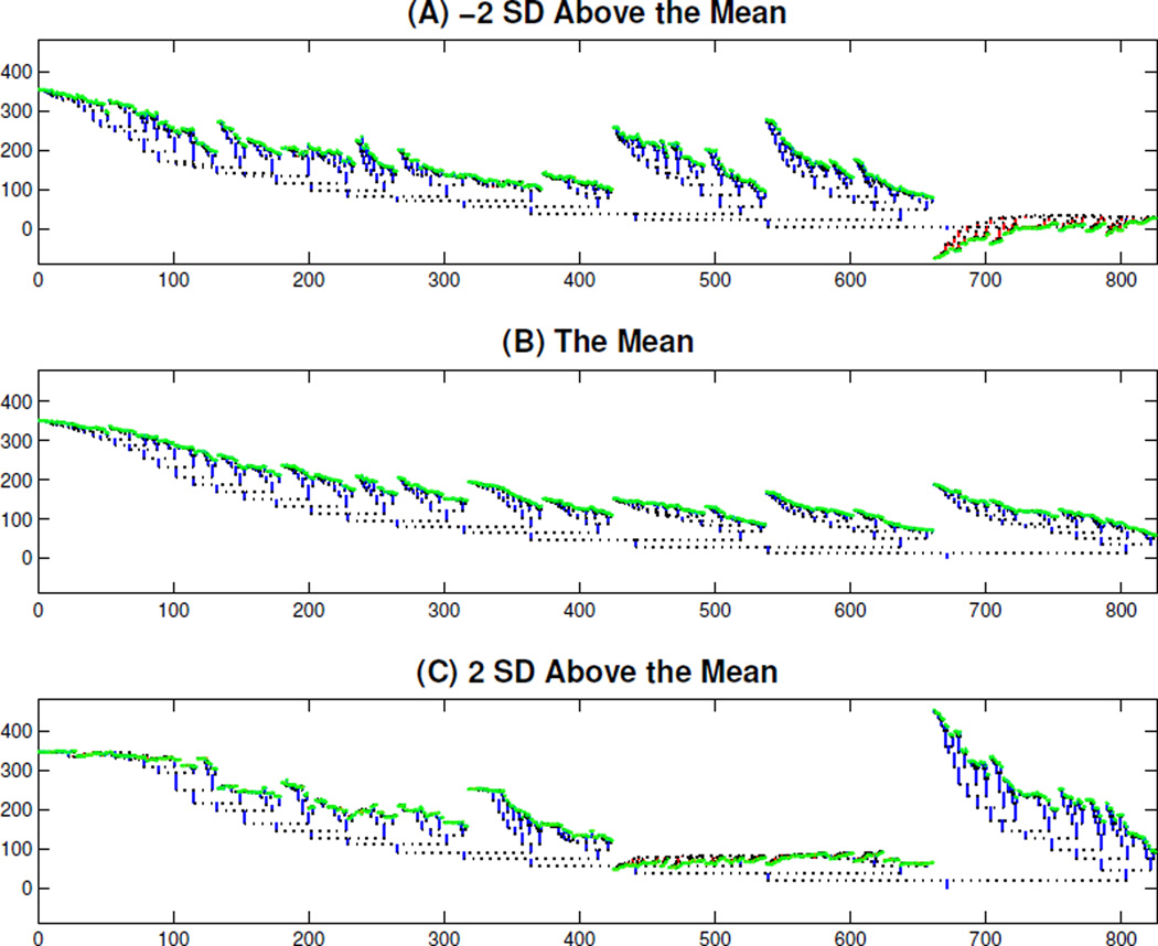
Illustration of PC1 Mode of Variation in Binary Tree Space. Binary trees from top to bottom corresponding to the points on the PC1 direction vector, which are −2, 0, and +2 standard deviations distance above mean respectively. The red branches indicate negative length. Thus some are not valid binary trees, i.e., this linear representation of the data leaves the tree space.

In Figure 9, we take a deeper look at this PC1 mode of variation, in terms of the original trees. Assume that σ is the standard deviation of the PC1 projected scores s_1,1, ⋯ , s_n,1. The trees from top to bottom correspond to three points X̅ + 2kσu₁, k = − 2, 0, 2, on the PC1 direction vector, which are −2, 0, and +2 standard deviations above the mean, respectively. These trees show that most of the variation in the PC1 direction is due to branches in the right part of the trees. This is consistent with Panel (B) of Figure 8, which shows that most variation happens in the right part of the DPR curves. Figure 9 illustrates an important issue for PCA in Dyck path space: some of the branch lengths are negative, as shown in red, i.e. the PC reconstructions are no longer in the tree space. A natural attempt at fixing this problem is to do PCA on the logs of the DPR, and then exponentiate the results. This was attempted, but failed, because construction of the tree representations in Figure 9 is based on differences of cumulative lengths, which again were occasionally negative. A second unappealing aspect of the trees shown in Figure 9 is that they have essentially no flat parts (missing branches) which are very different from each population tree, as shown in Figure 4. A promising approach to address both of these issues, to be explored in future work, is nonnegative matrix factorization (NMF) (Lee and Seung, 2001).

4.2 SiZer Analysis

Another interesting phenomenon is found by studying the PC scores s_i,1 in (1), i.e. projections of the data onto the first eigenvector, as shown in Panel (A) of Figure 10. The green points are the scores, shown as a jitter plot using a vertical coordinate representing order in the data set, to avoid overplotting. Distributional properties of the scores s_1,1, ⋯ , s_n,1 are highlighted by overlaying (in Panel (A)) Gaussian kernel density estimates, i.e. smooth histograms, shown in blue. These curves are indexed by the smoothing parameter. They suggest that the distribution is bimodal for bandwidths around 10^3.1, shown as the thick line type in Panel (A) of Figure 10.

Figure 10.

SiZer Analysis of PC1 Projection Scores. Panel (A) is a family of kernel density estimates, with one curve highlighted as a thick line. The range of bandwidths for the family of estimated curves is shown on the log scale vertical axis of Panels (B) and (C), the SiZer (curvature) maps, where the y-value of the black horizontal line corresponds to the log scale bandwidth of the highlighted curve in Panel (A). The colors in the SiZer (curvature) maps assess the statistical significance of the bimodal distribution of the highlighted curve in Panel (A), showing that it is not a noise artifact.

To investigate whether the apparent bimodal structure is important, as opposed to a mere sample artifact, the latest version of SiZer (Hannig and Marron, 2006) is applied. First, the slope SiZer Map in Panel (B) analyzes the slope of the kernel density estimates.

This SiZer map uses the same x-coordinate values as in Panel (A). The y-coordinate value of the SiZer map corresponds to log scale bandwidths of the estimated curves in Panel (A), where the height of the black horizontal line corresponds to the highlighted curve in Panel (A). In addition, the extreme (roughest and smoothest) curves in Panel (A) correspond to the smoothing parameters whose log scales are the low and up boundaries of y-coordinate in Panel (B). The blue (red) color in the SiZer map means that the corresponding smooth curve in Panel (A) has significantly positive (negative) slope on the corresponding x-coordinate region. The purple color means the slope is not significant, and the gray color means that the data is too sparse to generate a meaningful result. The SiZer map does not indicate statistically significant bimodality in any of the kernel estimates because there is no kernel estimate whose bandwidth lines can pass through blue-red-blue-red regions in Panel (B).

For a deeper investigation, we use the curvature SiZer map (see Hannig and Marron (2006)) in Panel (C) of Figure 10 to study the statistical significance of the curvature of the kernel estimates to study their bimodal property. The curvature map has the same x and y-coordinate values as the SiZer map in Panel (B). The cyan (orange) color in the curvature map means that the corresponding smoothing curve in Panel (A) has statistically significant convex (concave) curvature on the corresponding x-coordinate region. The green color means the curvature is not significant, and the gray color means that the data is too sparse to generate a significant result. The black horizontal line passing through cyan-orange-cyan regions in the curvature map establishes the statistical significance of the bimodal distribution of the thick black curve in Panel (A). The curvature SiZer map in Panel (C) finds significant bimodality, which is not found by the slope SiZer map. This might seem like a contradiction, but is not, because the two different SiZer approaches take quite different views of modality, and thus can give different results. E.g. when a right hand true underlying mode is much taller than a true left hand mode, the processing of smoothing can eliminate the significance of the downward slope of the left mode. Curvature SiZer is very valuable because it tends to find such features. A direct analog of this phenomenon is the field of distribution testing, where one test is more powerful against some alternatives, and other tests are more powerful against others.

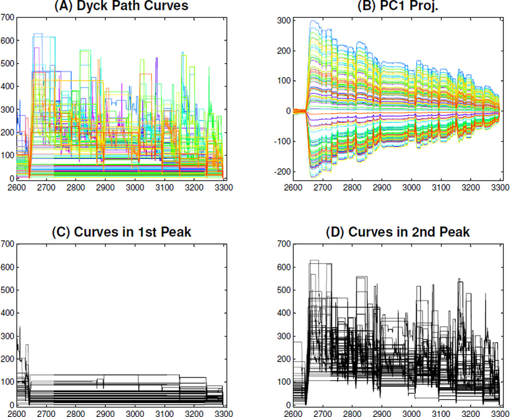
While the SiZer analysis is suggestive, it is based on several crude assumptions, and approximations. For example, while PC scores have provided many interesting insights over the years, they can also obscure important structure. These are additionally suspect, because as we showed in Section 4.1, some of these lead to invalid projected trees. Hence, a deeper look is needed both to check on this issue, and also to try to understand what is driving this observed phenomenon. To explore the reason for this bimodal distribution, recall from Panel (B) in Figure 8 that most of this dominant component of variation is on the right side. Hence we zoom in on this region (entries 2600–3300) in Figure 11. The zoom of the original DPR curves are shown in Panel (A) and the zoomed PC1 projections are in Panel (B). The bimodality shows up as a reduced density of curves near the middle of Panel (B). Panel (A) gives a suggestion of the reason: there are many curves which are quite flat, and others which have much more structure, i.e. contain relatively few flat parts.

Figure 11.

Zoomed DPR Curves. The first row plots show a zoomed-in version of the first row plots from Figure 8, where the zoomed part highlights the main variation part in the PC1 direction. The second row plots separate the two groups of the zoomed DPR curves, where the PC1 projection scores of the first (second) group, shown in the left (right) panel, are below (above) the local minimum point between the two peaks of the black thick curve in Panel (A) of Figure 10.

To investigate whether this two group phenomenon drove the main mode of variation in the DPR curves and thus the bimodal PC1 scores distribution, we split the DPR curves into two groups using the (middle) local minimum of the thick black curve in Panel (A) of Figure 10. The group to the left of the minimum is shown in Panel (C) of Figure 11. The group of curves to the right of the minimum is shown in Panel (D) of Figure 11. Note that the curves in Panel (D) have a large amount of structure, indicating trees with full branches on both sides of the first split. This dichotomy of the population was a surprise, instead a continuum between these extremes (of medium sized minor branches at the first split) was expected. This phenomenon appeared only for the back trees, and motivated further anatomical study.

4.3 Relationships with Age and Gender

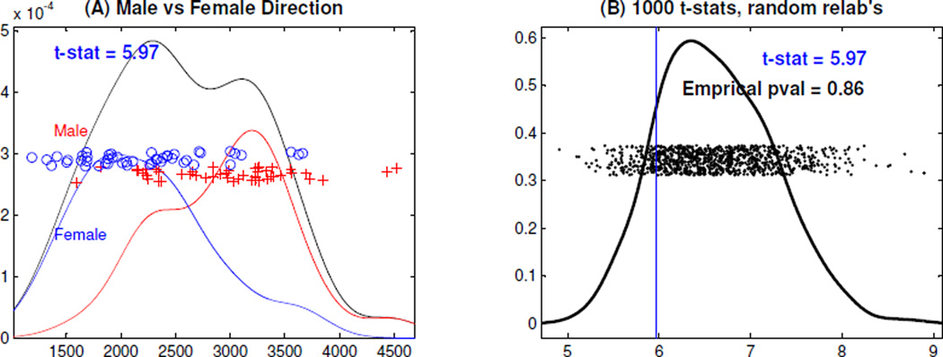
Also of interest is the effect of gender and age on tree topology. First we explore this relationship using the DPR. Gender difference can be highlighted using discrimination methods. Distance weighted discrimination (DWD) in Marron et al. (2007); Qiao et al. (2010) is an efficient tool to study population differences, especially in high dimensions. We project the DPR curves onto the DWD direction, and explore the projection scores in Panel (A) of Figure 12. The colored curves are rescaled kernel estimates of the male and female sub-population, respectively, whose areas are proportional to their relative sample size. Panel (A) suggests that the males have bigger mean DWD scores than the females. A naive look into this would use the 2-sample t-test statistic of 5.97, for the average difference between the male and female DWD scores. This is inappropriate, because the DWD direction makes this difference as large as possible. As shown in Wei et al. (2012), even when there is no actual difference, the t-test statistic computed on such projections can be much larger than the conventional t critical value.

Figure 12.

DiProPerm Test on the DWD Scores. Panel (A) shows the kernel density estimates for the male (red), the female (blue), and the union (black) curves. Panel (B) is the kernel density estimate of the 1000 t-stats, generated by the 1000 random permutations, and shows the empirical p-value indicating no statistical significance.

To properly assess significance, we used the DiProPerm test, described in Wichers et al. (2007) and Wei et al. (2012). The DiProPerm test uses a random permutation of the class labels to split the data into two groups, e.g. the male and female groups, and the DWD direction is recomputed for the relabeled data. For each random permutation, we calculated the 2-sample t-test statistic for the male and female DWD scores, and the statistic values are shown as the black dots in Panel (B) of Figure 12. The empirical p-value, which is essentially the percentage of random t-test statistic values greater than the real value, is shown in Panel (B). The DiProPerm empirical p-value (0.86) implies that the DWD projection scores actually show no significant difference between male and female. However, Panel (A) suggests the potential for finding some difference between males and females that will be reconsidered from a different viewpoint in Section 5.2.

We have similarly explored relationship with age, using partial least squares (PLS) (Wold et al., 1984), and canonical correlation analysis (CCA) (Häardle and Simar, 2007). Nothing significant are found in the analysis so results are not shown here. We refer the reader to Shen (2012) for a more descriptive narration of the analysis.

We also applied FDA to the log scale DPR curves to similarly explore the variation, and the gender/age effects. As seen in Chapter 4 of Shen (2012), the results are very similar to those obtained when analyzing the original scale. The square root transform was also considered, again with similar results. We have explicitly presented the original data scale here, as this represents the most natural units.

4.4 Branch Length Analysis

Note that the DPR uses only the cumulative lengths of the branches, and neglects the individual branch length information. In order to directly focus on individual branch length information, the BLR representation introduced in Section 3.3 is very useful. A BLR analysis, similar to the above, can be found in Chapter 4 of Shen (2012) who studied the variation of the BLR curves, using PCA, DiProPerm, PLS and CCA in a parallel analysis to that of Section 4. Results are quite similar, so they are not given explicitly here. Important differences between DPR and BLR do come up in Section 4.6 of Shen (2012), where it is seen that both give important insights.

5 Tree Pruning

5.1 Level k Pruned Support Tree

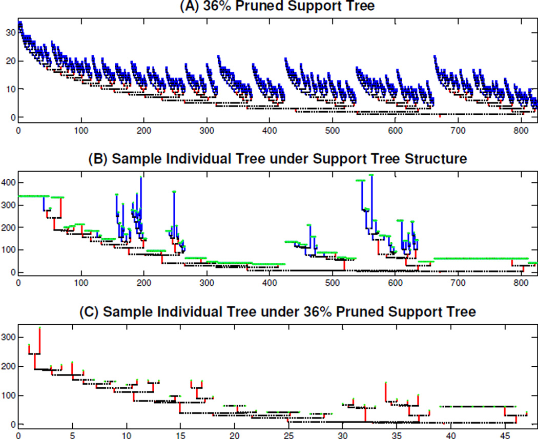
Under the support tree structure, each data tree has a large number of missing branches, as shown in Figure 4, which brings many challenges to the statistical analysis. To address these challenges, we develop the concept of tree pruning. For a percentage k, the k% pruned support tree is the union of the individual trees’ branches that appear in at least k percent of the individual trees. For illustration purposes, the red tree in the top panel of Figure 13 is the 36% pruned support tree. The focus here is on topological structure, so all branch lengths are set to be 1.

Figure 13.

Illustration of Tree Pruning, for Support Tree and an Individual. The red tree in Panel (A) is the 36% pruned support tree whose branches appear in at least 36 percent of the individual trees. Panel (B) is an individual tree under the support tree structure, where the missing branches are colored green, the non-missing branches that appear in the 36% pruned support tree are red, and the non-missing branches that are not in the pruned support tree are blue. Panel (C) is the corresponding individual 36% pruned tree that contains the red branches and the missing branches that appear in the 36% pruned support tree in the top panel.

For each pruning level, we define individual pruned trees. Assume that each individual tree has been put into the support tree structure, as in Figure 4. Panel (B) of Figure 13 shows one individual tree (case number i = 1) under the support tree structure, where the flat parts are a sequence of green points, each representing a missing branch. The non-missing branches that appear in the 36% pruned support tree are colored red, and the non-missing branches that do not appear in the 36% pruned support tree are colored blue. Panel (C) shows the individual 36% pruned tree. This keeps the red branches, and those missing branches that are present in the 36% pruned support tree in Panel (A). Note that many missing branches in Panel (B) of Figure 13 disappear under the pruned support tree structure, as indicated by the range of the horizontal axis.

Figure 13 shows that the tree pruning operation tends to prune off fine scale clusters of higher level branches, that are shared by relatively few other trees. Thus the pruned analysis tends to focus on widely shared global population properties.

Recall that the descendant correspondence method puts the branch that has more descendant branches to the left, and the trees in Figure 2 and 4 have the descendant correspondence property. We now show that the individual pruned trees, e.g. the one shown in the bottom panel of Figure 13, also have this property. Note that the k% pruned support tree, e.g. the red tree in Panel (A) of Figure 13, has the descendant correspondence property.

Theorem 1 Each k% pruned support tree keeps the descendant correspondence property

The proof of Theorem 1 is skipped here to save space, see details in Section 4.6 of Shen (2012). Since individual pruned trees have the same branches as the pruned support tree, it follows from Theorem 1 that the individual pruned trees have the descendant correspondence property.

Next we discuss details of the pruned tree analysis. The results were not radically different between the DPR and BLR approach. They were a little more compelling for the latter, so a more detailed summary of the branch length results appears in Section 5.3. A short verbal summary of the DPR analysis appears in Section 5.2.

5.2 Pruned Dyck Path Analysis

The pruned support tree structure decreases the number of missing branches of individual trees, and can help improve the efficiency of the statistical analysis. As we did in Section 3.2, we first transform the individual pruned trees to the DPR curves. These DPR curves still have some flat parts because the individual pruned trees still have a few missing branches. The left part of the DPR curves appears higher than right because of the descendant correspondence property of the individual pruned trees.

As in Section 4, we used DiProPerm to study gender differences of the DPR curves at different pruning percentages 1%, 6%, ⋯ , 96% of the back, front, left, and right trees. This fairly large array of hypothesis tests resulted in statistical significance (level 0.05) only near the pruning percentage 21% for the right tree. Using an appropriate multiple comparison approach, the False Discovery Rate (FDR) (Benjamini and Yekutieli, 2001), left no clear statistical significance. Further details can be found in Shen (2012).

5.3 Pruned Branch Length Analysis

We applied the PCA visualization technique, as well as the DiProPerm gender hypothesis test, on the BLR of the pruned trees. Most results were similar to those in Sections 4, 4.4 and 5.2, and are not repeated here (details can be found in Shen (2012)). What we describe here is the analysis of age and gender effect on the trees.

5.3.1 Age Effect

We now study the relationship between age and some summaries introduced in Section 1. These include total branch length (TBL), average branch length (ABL), and the number of non-missing branches (NNB) of each individual pruned tree.

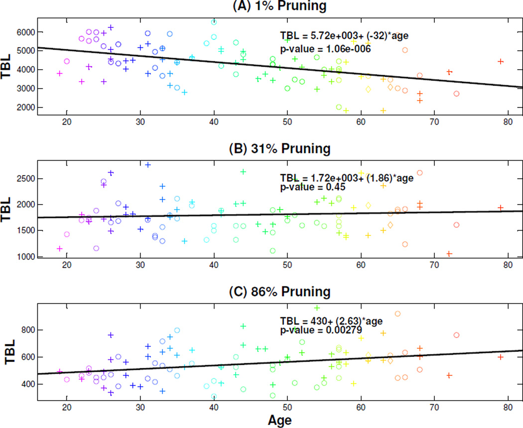
Figure 14 shows scatterplots for different pruning levels, where TBL (age) are the corresponding y (x) coordinates. Panel (A) shows the scatterplot without pruning. The same age based rainbow coloring system from Figures 7, 8, and 11 is used here. The symbols plus, circle and diamond correspond to males, females, and transgenders respectively. It appears that TBL has a negative relationship with age. As the pruning level increases, the scatterplots in Panels (B) and (C), corresponding to the 31% and 86% pruning respectively, suggest that the negative relationship disappears.

Figure 14.

Scatterplots Exploring the Relationship between TBL of Individual Pruned Trees (back) and Age of Samples. Color and symbol code are as before for age and gender, respectively. The top, middle, and bottom panels correspond to the 1%, 31%, and 86% pruning respectively. The solid line in each panel is an estimated linear regression line. Slope hypothesis tests show a significant decreasing effect for 1% pruning and increasing slope for 86%.

To further investigate this phenomenon, we carry out a linear regression analysis. Note that the slope values change from negative (Panel (A)) to positive (Panels (B) and (C)). Furthermore, the statistical significance of the slopes change from significantly negative in Panel (A) to not significant in Panel (B) and significantly positive in Panel (C). Thus the age relationship for TBL ranges from negative to positive, as the pruning level increases. We used FDR to perform a multiple comparison analysis, and the linear regressions in Panels (A) and (C) remain significant (q-value = 0.05). The analysis was done over the range of pruning percentages 1%, 6%, ⋯ , 96%. Figure 14 shows the plots for just 1%, 31%, 86%, chosen to represent three different relationships between TBL and age.

In personal discussion, Dr. E. Bullitt, the neuroscientist who collected the brain data, explained that older people suffer occasional brain artery blockage. But often these vessels are too small to appear in the MRA, so older people tend to have overall shortened TBL as seen in the top panel of Figure 14. When the branches are pruned down to common branches only, these tend to be longer for older people, because of this compensation.

Similar analysis for the other brain regions only found partially significant results, see Shen (2012) for details.

5.3.2 Gender Relationship

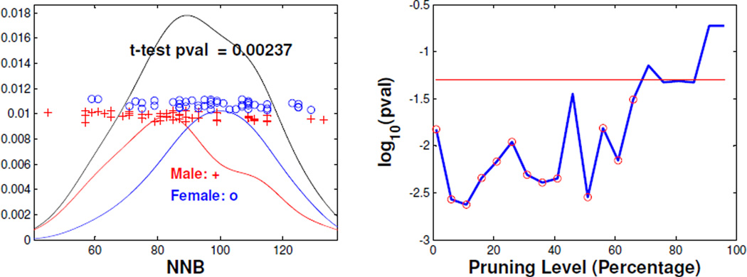
Similar to the analysis of Section 4.3, we now apply DiProPerm to study gender effects for the BLR pruned trees. The plus (red) and circle (blue) symbols in the left panel of Figure 15 represent the NNB scores of individual (right side) 11% pruned trees, for males and females respectively. The left panel also shows the kernel density estimate for the male (red), the female (blue), and the union (black) curves. The male and female kernel estimates suggests that females have larger NNB scores than males. This motivated a two sample t-test which found that females have significantly larger NNB scores than males (p-value = 0.002).

Figure 15.

Gender Difference Analysis for Individual (right side) Pruned Trees. The left panel shows the kernel estimates of NNB (11% pruning) for male (red), female (blue) and their union (black), and the t-test analysis. The right panel is a log scale p-value plot, where the x-coordinate is pruning level. The red horizontal is the significant line (p-value = 0.05) and the red circles correspond to the significant (q-value = 0.05) pruning levels after multiple comparison adjustment.

The two-sample t-test is next performed over a wide range of pruning levels. For pruning percentage 1%, 6%, ⋯ , 96%, their corresponding log scale p-values are plotted in the right panel in Figure 15. The red horizontal line corresponds to p-value = 0.05. Note that most parts of the p-value curve are below the red line. This suggests that the corresponding NNB is significantly different between males and females under the corresponding pruning level. Here, we also used FDR to do multiple comparison analysis and the finally significant (q-value = 0.05) pruning levels are highlighted by red circles. This further confirms that NNB is significantly different between males and females for most pruning levels. Explanation of this new discovery is an open problem in anatomy.

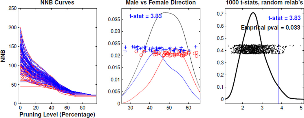
In the above analysis, the data objects were individual pruning levels and significant gender difference in NNB were found for most pruning levels. Next, we consider totally different data objects, which are the NNB scores as a function of pruning level. Such curves as data are amenable to FDA. DiProPerm then gives another approach to gender difference analysis.

The left panel in Figure 16 shows the NNB curves, i.e. new data objects, for the right side trees, where the x-coordinate is the pruning levels and the y-coordinate is the NNB score. The red and blue curves correspond to males and females respectively. We then applied the DiProPerm test (the middle and right panels) to the curves. The empirical p-value (0.033) in the right panel suggests a significant difference between the male and female groups for NNB.

Figure 16.

Global Gender Analysis. The left panel shows the NNB curves for (right) trees, where the x-coordinate is the pruning level and the y-coordinate is the NNB score. The middle panel shows the kernel density estimate for male (red), female (blue), and the union (black). The right panel is the kernel density estimate of the 1000 t-stats, generated by the 1000 random permutations, along with the empirical p-value indicating statistical significance.

Similar analysis on TBL and ABL and other brain regions only found partially significant results, see Shen (2012) for details.

6 Discussion

This paper approached the statistical analysis of a data set of tree structured data objects using various representations. The first, called Dyck Path, was motivated by an idea from probability theory. This led to invention of a second representation, called Branch Length, which highlighted different interesting aspects of the data. Both representations allowed direct application of FDA methods, such as PCA, which gave a number of interesting insights about the the data. Unsatisfactory aspects of these representations were addressed with a novel noise reduction method called Tree pruning, which led to additional insights.

One avenue for future work was shown in Figure 9 where standard PCA representations left the tree space in interesting regions. Appropriate modifications of NMF are well worth exploring. A quite different approach would be the Bayes factor analysis approach, as in Kim and Lee (2003). Another approach to tree data analysis would be to use the large body of knowledge called phylogenetic trees, see Billera et al. (2001). A major challenge to this approach is that it requires all trees in the data set to have a common, corresponding set of leaves (species in classical phylogenetics). An approach to this, based on sophisticated image analysis ideas, is currenly under study.

One more direction of potential future improvement is in the direction of the correspondence issue, addressed in Section 2.1. It would be interesting to address this through an equivalence relation, as in Feragen et al. (2010).

References

- Aydin B, Pataki G, Wang H, Bullitt E, Marron J. A principal component analysis for trees. The Annals of Applied Statistics. 2009;3(4):1597–1615. [Google Scholar]
- Aydin B, Pataki G, Wang H, Ladha A, Bullitt E, Marron J. Visualizing the structure of large trees. Electronic Journal of Statistics. 2011;5:405–420. [Google Scholar]
- Aydin B, Pataki G, Wang H, Ladha A, Bullitt E, Marron J. New approaches to principal component analysis for trees. Statistics in Biosciences. 2012;4:132–156. [Google Scholar]
- Aylward S, Bullitt E. Initialization, noise, singularities, and scale in height ridge traversal for tubular object centerline extraction. IEEE Transactions on Medical Imaging. 2002;21(2):61–75. doi: 10.1109/42.993126. [DOI] [PubMed] [Google Scholar]
- Benjamini Y, Yekutieli D. The control of the false discovery rate in multiple testing under dependency. The Annals of Statistics. 2001;29(4):1165–1188. [Google Scholar]
- Billera L, Holmes S, Vogtmann K. Geometry of the space of phylogenetic trees. Advances in Applied Mathematics. 2001;27(4):733–767. [Google Scholar]
- Collins M, Duffy N. Convolution kernels for natural language. In Proceedings of NIPS. 2001;Volume 14:625–632. [Google Scholar]
- Dryden I, Mardia K. Statistical shape analysis. Volume 4. New York: Wiley; 1998. [Google Scholar]
- Dumoulin C, Hart H. Magnetic resonance angiography. Radiology. 1986;161(3):717–720. doi: 10.1148/radiology.161.3.3786721. [DOI] [PubMed] [Google Scholar]
- Eom J, Kim S, Kim S, Zhang B. A tree kernel-based method for protein-protein interaction mining from biomedical literature. Knowledge Discovery in Life Science Literature. 2006;3886:42–52. [Google Scholar]
- Feragen AF, Lauze P, Lo M, de Bruijne Nielsen M. Geometries on spaces of treelike shapes. Computer Vision-ACCV. 2010;2010:160–173. [Google Scholar]
- Ferraty F, Vieu P. Nonparametric functional data analysis: theory and practice. Verlag: Springer; 2006. [Google Scholar]
- Handle. 2008 Tree Data, “ http://hdl.handle.net/1926/594”.
- Hannig J, Marron J. Advanced distribution theory for sizer. Journal of the American Statistical Association. 2006;101(474):484–499. [Google Scholar]
- H¨ardle W, Simar L. Applied Multivariate Statistical Analysis. Verlag: Springer; 2007. [Google Scholar]
- Harris T. First passage and recurrence distributions. Transactions of the American Mathematical Society. 1952;73:471–486. [Google Scholar]
- Jolliffe I. Principal component analysis. Verlag: Springer; 2002. [Google Scholar]
- Kim Y, Lee J. Bayesian bootstrap for proportional hazards models. The Annals of Statistics. 2003;31(6):1905–1922. [Google Scholar]
- Lee D, Seung H. Algorithms for non-negative matrix factorization. Advances in neural information processing systems. 2001;13:556–562. [Google Scholar]
- Marron J, Todd M, Ahn J. Distance-weighted discrimination. Journal of the American Statistical Association. 2007;102(480):1267–1271. doi: 10.1198/jasa.2010.tm08487. [DOI] [PMC free article] [PubMed] [Google Scholar]
- Qiao X, Zhang H, Liu Y, Todd M, Marron J. Weighted distance weighted discrimination and its asymptotic properties. Journal of the American Statistical Association. 2010;105(489):401–414. doi: 10.1198/jasa.2010.tm08487. [DOI] [PMC free article] [PubMed] [Google Scholar]
- Ramsay J, Silverman B. Applied functional data analysis: methods and case studies. Verlag: Springer; 2002. [Google Scholar]
- Ramsay J, Silverman B. Functional data analysis. Verlag: Springer; 2005. [Google Scholar]
- Shawe-Taylor J, Cristianini N. Kernel methods for pattern analysis. Cambridge Univ Pr.; 2004. [Google Scholar]
- Shen D. Sparse PCA asymptotics and analysis of tree data. Ph.d Thesis, Department of Statistics and Operations Research, University of North Carolina at Chapel Hill. 2012 [Google Scholar]
- Shen D, Shen H, Marron JS. Consistency of sparse PCA in high dimension, low sample size contexts. Journal of Multivariate Analysis, forthcoming. 2012 [Google Scholar]
- Vert J. A tree kernel to analyse phylogenetic profiles. Bioinformatics. 2002;18(suppl 1):276–284. doi: 10.1093/bioinformatics/18.suppl_1.s276. [DOI] [PubMed] [Google Scholar]
- Wang H, Marron J. Object oriented data analysis: Sets of trees. The Annals of Statistics. 2007;35(5):1849–1873. [Google Scholar]
- Wei S, Lee C, Wichers L, Li G, Marron J. Direction-projection-permutation for high dimensional hypothesis tests. Tech. Rep., Department of Statistics and Operations Research, University of North Carolina at Chapel Hill. 2012 [Google Scholar]
- Wichers L, Lee C, Costa D, Watkinson W, Marron J. A functional data analysis approach for evaluation temporal physiologic responses to particualate matter. Tech. Rep. 5, Department of Statistics and Operations Research, University of North Carolina at Chapel Hill. 2007 [Google Scholar]
- Wold S, Ruhe A, Wold H, Dunn III W. The collinearity problem in linear regression. The partial least squares (PLS) approach to generalized inverses. SIAM Journal on Scientific and Statistical Computing. 1984;5(3):735–743. [Google Scholar]
- Yamanishi Y, Bach F, Vert J. Glycan classification with tree kernels. Bioinformatics. 2007;23(10):1211–1216. doi: 10.1093/bioinformatics/btm090. [DOI] [PubMed] [Google Scholar]
- Yao F, Mu¨ller H, Clifford A, Dueker S, Follett J, Lin Y, Buchholz B, Vogel J. Shrinkage estimation for functional principal component scores with application to the population kinetics of plasma folate. Biometrics. 2003;59(3):676–685. doi: 10.1111/1541-0420.00078. [DOI] [PubMed] [Google Scholar]
Associated Data
This section collects any data citations, data availability statements, or supplementary materials included in this article.