Detecting Pairwise Correlations in Spike Trains: An Objective Comparison of Methods and Application to the Study of Retinal Waves

Abstract

Correlations in neuronal spike times are thought to be key to processing in many neural systems. Many measures have been proposed to summarize these correlations and of these the correlation index is widely used and is the standard in studies of spontaneous retinal activity. We show that this measure has two undesirable properties: it is unbounded above and confounded by firing rate. We list properties needed for a measure to fairly quantify and compare correlations and we propose a novel measure of correlation—the spike time tiling coefficient. This coefficient, the correlation index, and 33 other measures of correlation of spike times are blindly tested for the required properties on synthetic and experimental data. Based on this, we propose a measure (the spike time tiling coefficient) to replace the correlation index. To demonstrate the benefits of this measure, we reanalyze data from seven key studies, which previously used the correlation index to investigate the nature of spontaneous activity. We reanalyze data from β2(KO) and β2(TG) mutants, mutants lacking connexin isoforms, and also the age-dependent changes in wild-type and β2(KO) correlations. Reanalysis of the data using the proposed measure can significantly change the conclusions. It leads to better quantification of correlations and therefore better inference from the data. We hope that the proposed measure will have wide applications, and will help clarify the role of activity in retinotopic map formation.

Introduction

Quantifying the degree of correlation between neural spike trains is a key part of analyses of experimental data in many systems (Chiappalone et al., 2006; Dehorter et al., 2012; Kirkby et al., 2013). Neural coordination is thought to play a key role in information propagation and processing and also in self-organization of the neural system during development. For example, correlated activity plays a critical role in forming the retinotopic map (Feller, 2009). In the developing retina, waves of correlated spontaneous activity in retinal ganglion cells have been recorded [on multielectrode arrays (MEAs) and by calcium imaging] in vitro in many species (Wong, 1999), and shown in vivo using calcium imaging in mouse (Ackman et al., 2012). These waves show both temporal and spatial correlations. Much work has focused on assessing the role of this activity in the development of the retinotopic map; typically, both the map and various statistics of the activity are compared between wild-type and mutant genotypes. The results are used to make inferences about which features of the activity are implicated in retinotopic map formation (Stafford et al., 2009). There is strong evidence that correlation between neuronal spike times is involved in this process (Xu et al., 2011).

An appropriate quantification of these correlations is vital for inference about their role. Quantifying correlations is challenging for two reasons. First, correlated neurons fire at similar times but not precisely synchronously, so correlation must be defined with reference to a timescale within which spikes are considered correlated. Second, spiking is sparse with respect to the recording's sampling frequency (spiking rate ∼1 Hz, sampling rate typically 20 kHz; Demas et al., 2003) and also spike duration. This means that conventional approaches to correlation (such as Pearson's correlation coefficient) are unsuitable as periods of quiescence should not count as correlated and correlations should compare spike trains over short timescales, not just instantaneously.

Many alternative measures of quantifying correlations exist (Kruskal et al., 2007; Kerschensteiner and Wong, 2008; Joris et al., 2006). One measure, the correlation index (Wong et al., 1993), has widespread popularity and is the standard measure applied to spontaneous retinal activity. It also has wider uses such as quantifying correlations in motor (Personius et al., 2007) or hippocampal (MacLaren et al., 2011) neurons. It is a pairwise measure, which quantifies temporal correlations and is frequently used to investigate their dependency on a third variable, such as neuronal separation, and to compare correlations across phenotypes. We show that the correlation index is confounded by firing rate, which means it cannot fairly compare correlations. We list properties required of a correlation measure and conduct a thorough literature search for other measures. We propose a novel measure and then blindly and systematically test all measures for the required properties against synthetic and experimental data to propose a replacement for the correlation index. Using this replacement, we then reanalyze data from seven studies to show that results can change when correlations are measured in a way that is independent of firing rate.

Materials and Methods

Analysis of correlation index

The correlation index i_A,B between two spike trains A and B is defined as the factor by which the firing rate of neuron A increases over its mean value if measured within a fixed window (typically 0.05–0.10 s) of spikes from neuron B (Wong et al., 1993). The following notation is used throughout: the vectors a and b represent the spike times of neurons A and B; a_i is the i′th spike in train A and b_j is the j′th spike in train B. The correlation index is given by the following:

where N_A = |a| (total number of spikes of A in recording, N_B = |b|, T = length of recording, Δt = synchronicity window, and N_A,B[−Δt, Δt] is the number of spike pairs where a spike from train A falls within ±Δt of a spike from train B as follows:

where

To show that the correlation index is dependent on firing rate, we assume the following model for neuronal firing: spike trains A and B are both Poisson processes with rates λ_A and λ_B respectively. A fixed proportion of the spike times are shared (A and B fire spikes synchronously). These synchronous spikes occur with a rate λ_S ≤ λ_A, λ_B. Adjusting these parameters can scale the rates while maintaining the correlation structure to test for rate-dependence. Under this model, an expression for the correlation index can be derived as follows:

This expression is clearly rate-dependent. Two minor assumptions about the size of the rates, T and Δt were used to arrive at this result. These assumptions are valid within experimentally observed ranges and the rate-dependency of i_A,B is not affected if the assumptions are violated. In Results, we use the subcase of autocorrelation λ = λ_A = λ_B = λ_S to show that this rate-dependence significantly affects correlation values. In this case, the correlation index is as follows:

This dependency was verified computationally by extensive testing on synthetic data, including data generated from the above model using freely available code (Macke et al., 2009).

Spike time tiling coefficient

We define the spike time tiling coefficient in Figure 1. To quantify the correlation between spike trains A and B, we look for spikes in A which fall within ±Δt of a spike from B. We consider the proportion of spikes in A which have this property as this is insensitive to firing rate. We account for the amount of correlation expected by chance by making the minimal assumption that we expect the proportion of spikes from A falling within ±Δt of a spike from B by chance to be the same as the proportion of the total recording time which falls within ±Δt of a spike from B. Any extra spikes in A which have this property are indicative of positive correlation. We therefore use the quantity P_A − T_B (Fig. 1 shows definitions) which is positive if spikes in train A are correlated with spikes from train B, and negative if there is less correlation than expected by chance. We require the coefficient to be equal to +1 for autocorrelation, to be −1 when P_A = 0, T_B = 1 and to have a range of [−1, 1]. The normalization factor (1 − P_AT_B) ensures that these criteria hold.

Figure 1.

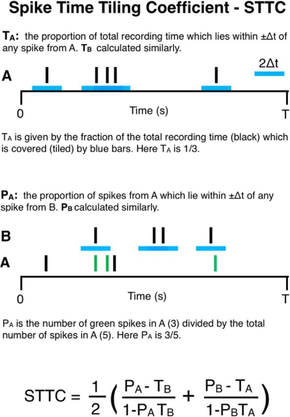
Diagram to demonstrate the calculation of the spike time tiling coefficient. The four quantities required to calculate the spike time tiling coefficient are P_A, P_B, T_A, T_B. The only free parameter is Δt. Values and scales are for demonstration only.

The coefficient should be symmetric so we consider both (P_A − T_B) and (P_B − T_A), combine the contributions from both trains and renormalize to preserve the required range (Fig. 1). Computation of the spike time tiling coefficient is straightforward; the only complexity is ensuring that overlapping tiles do not count multiple times when calculating T_A and T_B.

The spike time tiling coefficient uses the proportion of the recording which falls within ±Δt of spikes from A to determine whether the proportion of spikes in B which also have this property is indicative of correlation (i.e., more or less than is expected by chance). Because tile overlaps are not counted multiple times, this depends on the firing patterns as well as rates. In the correlation index (and many other measures), only the firing rates are used to assess what is expected by chance, but firing patterns are, in fact, important. For instance, consider an extreme case of two spike trains (A and B) with the same average firing rate where the spikes in A occur at regular intervals (no two spikes are within Δt of each other) and the spikes in B all occur within Δt of each other. More of the recording time lies within ±Δt of any spike from A compared with B so given an arbitrary train C, we expect more spikes in C to fall within ±Δt of any spike from A by chance than within ±Δt of any spike from B. This information is not captured using the firing rates to assess what we expect to occur by chance but is captured with the spike time tiling coefficient.

Implementing the measures

A literature search produced 33 other measures that were implemented for testing. All measures were implemented in R and C except Victor and Purpura (1997), ISI-distance (Kreuz et al., 2007a), van Rossum (2001), and SPIKE (Kreuz et al., 2013), which were run using freely available MATLAB code (Kreuz et al., 2013). Some measures were altered to make them more likely to posses the required properties. The following changes were made (see Table 3): the Kerschensteiner and Wong (2008) and Jimbo et al. (1999) indices were originally defined as functions over binned time lags, the value of the bin around zero was taken to be the value of the measure (with bin width 2Δt). The Jimbo et al. (1999) index is normalized by the autocorrelation value at the origin, but the form of this normalization was not specified. Two versions of multiplicative normalization were tested, one used the above quantity, and the other used its square root. The requirement of the event synchronization measure (Kreuz et al., 2007b) that Δt should be smaller than the smallest within-train ISI was relaxed so Δt was set freely. The Schreiber et al. (2003) similarity coefficient and the Kruskal et al. (2007) correlation measure had their exponential/Gaussian filters (respectively) replaced with a boxcar filter of width 2Δt. This does not affect whether a measure fulfils the required criteria, but means that a window of synchrony is used to assess correlations (as with the correlation index). A boxcar filter is also more computationally efficient to calculate than Gaussian or exponential filters, which require an extra parameter, namely a filter cutoff point, to make computation feasible. Mutual information (Li, 1990) was altered to smooth spikes with a boxcar filter before calculation. The Ripley (1976) K_mm function (a directed measure which measures the correlation of one train to another) was made symmetric by setting the correlation measure to be equal to the mean of the two directed variants.

Table 3.

Correlation measures evaluated in this study with evidence (if any) for rejecting them as a replacement for correlation index

Measure no.	Measure name	Lacked property	Evidence in Figure
	Distance measures and cost functions
1	Victor and Purpura (1997)	N3	5A
2	ISI-distance (Kreuz et al., 2007a)	N2	5B
3	Hunter-Milton similarity (Hunter and Milton, 2003)	N6	5C
4	Van Rossum (2001)	N3	5A
5	SPIKE (Kreuz et al., 2013)	N2	5B
	Cross-correlation based
6	Coincidence index (Pasquale et al., 2008)	N2	4
7	Altered Coincidence index*	N2	4
8	Cross correlation coefficient (Pasquale et al., 2008)	N2	4
9	Schreiber et al. (2003) similarity coefficient	N6	5C
10	Altered Schreiber et al. similarity coefficient*	N6	5C
11	Kerschensteiner and Wong (2008) cross-correlation	D3	6D
12	Jimbo and Robinson index (Jimbo et al., 1999)	N2	4/5A
	Synchrony not from cross-correlation
13	Correlation index (Wong et al., 1993)	N2	3
14	Activity pair (Eytan et al., 2004)	N2	4
15	Unitary events analysis (Grün et al., 2002)	N2	4
16	Event synchronization (Kreuz et al., 2007b)*	N2	4
17	Joris et al. (2006) correlation index	N2	4
	Information theory
18	Mutual information (Li, 1990)	N2	4
19	Mutual information with smoothing*	N2	4
	Measures from shot-noise process
20	Coherence (at zero) (Eggermont, 2010)	N6	5C
21	Spike count correlation (Eggermont, 2010)	D1	6A
22	Smoothed spike count correlation (Kruskal et al., 2007)*	D3	6C
23	Spike count covariance (Eggermont, 2010)	N2	4
	Measures assuming a marked point process
24	Stoyan's Kmm function (Stoyan and Stoyan, 1994)	N2	4
25	Isham's mark correlation function (Isham, 1985)	N2	4
26	Ripley's Kmm function (Ripley, 1976)	N2	4
27	Simpson (1949) index	N2	4
28	Simpson (1949) index no correction	N2	4
29	Stoyan's mark covariance function (Stoyan, 1984)	N2	4
30	Mark variogram (Cressie, 1993)	N2	4
31	Mark covariance function (Cressie, 1993)	N2	4
32	Mark conditional expectation (E; Schlather et al., 2004)	N2	5B
33	Mark conditional variance (V; Schlather et al., 2004)	N2	4
34	Mark conditional standard deviation (Schlather et al., 2004)	N2	4
	Tiling-based
35	Spike time tiling coefficient	PASS

*Indicates that the measure was altered to make it applicable (see Materials and Methods).

All measures investigated are arranged according to our devised classification (see Materials and Methods). The third column contains an identifier (see Table 2) corresponding to one property, which the measure was shown to lack (if any). The fourth column denotes which figure presents evidence for the lacking property.

Evaluating the measures for the necessary and desirable properties

Each measure was tested extensively for the necessary and desirable properties (see Table 2) on a range of synthetic data. This was used instead of experimental data, as it is possible to independently alter the key properties (such as, rate or correlation). Synthetic data were generated from the following models, which replicate four types of experimentally observed spiking patterns: Poisson spiking, Poisson bursting, regular out-of-synchrony spiking, and out-of-synchrony bursting. Sample data are presented in Figure 2 and parameter ranges for all four models appear in Table 1.

Table 2.

Necessary (N) and desirable (D) properties for a correlation measure

Necessary properties

N1 Symmetry: The measure C should be symmetric: for spike trains A and B, C(A, B) = C(B, A).

N2 Robust to variations in the firing rate: For instance, given two spike trains with a particular correlational structure, if the rates of both trains are doubled but the structure is preserved, the correlation measure should remain the same.

N3 Robust to amount of data: In practice, this often means robust to recording duration.

N4 Bounded: The measure should be bounded taking a value of +1 when the spike trains are identical, with a value of zero corresponding to no correlation and −1 corresponding to anti-correlation.

N5 Robust to variations in Δt: Small variations to Δt should not introduce artefacts into the measure.

N6 Anticorrelation: The measure should discriminate between no correlation and anticorrelation.

Desirable properties

D1 Periods when both neurons are inactive should be ignored: Periods where both neurons are silent should not be counted as correlated. Experimental data frequently has large periods of quiescence (Wong et al., 1993; Demas et al., 2006) which, if counted would distort calculated correlations.

D2 Minimal assumptions on structure: The measure should not assume that spike times have a given underlying distribution as this will lessen the general applicability.

D3 Minimal Parameters: The main free parameter in the measure should be the time window of synchrony Δt. The number of other parameters should be kept to a minimum.

Each property is assigned an identifier for ease of reference.

Figure 2.

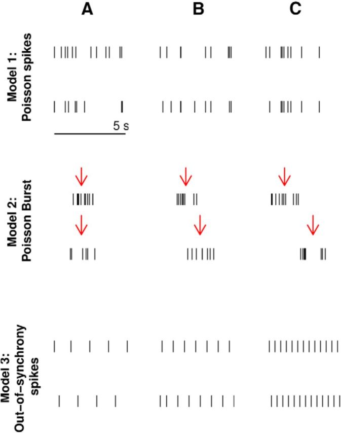
Examples of simulated data used to test measures. Data generated from Model 1 used a Poisson spiking model where both neurons fire at 1.5 Hz with increasing percentage of spike times which are shared with a spike in the other train: 0% (A), 87% (B), and 99% (C). Recording duration T = 300 s. Data generated from Model 2 used a Poisson burst model with a burst rate of λ = 0.05 Hz, where the number of spikes in each burst is drawn from a Poisson distribution with mean N = 8. The positions of the spikes relative to the center of the burst (indicated by a red arrow) are drawn from a uniform distribution on [−1, 1] s (σ = 2). The center of the burst of the second train is offset from the center of the first by a fixed amount: O = 0 s (A), 1 s (B), and 2 s (C), T = 3600 s. Data generated from Model 3 shows regular out-of-synchrony firing with increasing firing rate generated using an integrate-and-fire model (see Materials and Methods for details). The firing rates are 0.76 Hz (A), 1.27 Hz (B), and 2.5 Hz (C), T = 3000 s.

Table 1.

Parameter ranges used in models to generate test data

Parameter	Description	Value
	Common to all models
Δt	Window of synchrony	0.01–1 s
T	Recording time	10 to 6000 s
	Poisson spiking model
λA, λB	Firing rates of A and B	0.01–5 Hz
λS	Rate of synchronous spikes	0.01–5 Hz
	Poisson bursting model
λ	Burst-rate of master train	0.01–0.2 Hz
p	Probability of burst in second train	0–1
O	Parameter controlling offset of burst-center in second train (either fixed or O = range of continuous uniform distribution, or O = variance of Gaussian distribution)	0–2 s
N	Parameter controlling number of spikes per burst (either fixed, N = mean of Poisson distribution, or N = maximum of discrete uniform distribution)	1–20
σ	Parameter controlling position of spikes relative to burst center (σ = range of continuous uniform distribution, or σ = variance of normal distribution)	0.05–2 s
	Out-of-synchrony spiking model (Dayan and Abbott, 2001)
ES	Synapse reversal potential	−70 to 0 mV
EL	Resting potential	−70 mV
Vth	Threshold potential	−54 mV
Vreset	Reset voltage after action potential	−80 mV
τm	Membrane time constant	0.05–1.5 s
rmḡs	Specific membrane resistance multiplied by specific membrane conductance	0.05
Pmax	Maximum value of synaptic release probability	0.5
RmIe	Change in potential due to injection of small current	18 mV
τs	Synaptic time constant	0.05 s
	Out-of-synchrony bursting model (Shi and Lu, 2009)
α	Map control parameter	5–30
μ	Ensures slow gating process is slow	0.001
σA, σB, σC	Regime-control parameters for neurons A, B, C	−0.4 to −0.1
gc	Coupling strength	−0.4 to −0.01

Note that the out-of-synchrony bursting model is phenomenological, and so parameters do not relate to any particular biological process and are unitless.

Poisson spiking model.

This model assumes that spike trains A and B fire Poisson-distributed spikes with rates λ_A and λ_B, respectively. A certain proportion of these spikes are synchronous with a spike in the other train, this forms a Poisson process with rate λ_S. The rates, correlation, recording duration, and Δt were varied in isolation to test measures for the required properties.

Poisson burst model.

The Poisson burst model was used to generate data which replicated the burst-like firing seen in spontaneous retinal waves (a burst of firing when a cell participates in a wave and silence between waves). The model is a doubly stochastic process: the positions (center-points) of bursts are generated first, and then the bursts themselves (consisting of the number of spikes in the burst, and a position for each spike) are generated.

The first spike train is the “master” train and the center-points of its bursts are generated according to a Poisson process with a given rate λ. The center-points of the second train are a copy of those in the first train, but with some deleted (each center-point is deleted with probability, p). The remaining center points in the second train are then jittered from their initial positions. This is controlled by a parameter O which is either a fixed amount, the variance of a Gaussian distribution or the range of a continuous uniform distribution (in both cases the distributions have zero mean) from which the offsets are drawn.

For each center-point of a burst (in either train) the number of spikes in that burst is then generated. This is controlled by a parameter N which is either a fixed number or is the mean of a Poisson distribution or the maximum of a discrete uniform distribution from which the number of spikes are drawn. The position of each spike relative to the center-point is then generated and is controlled by a parameter σ which is either the variance of a Gaussian distribution or the range of a continuous uniform distribution (with zero mean in both cases) from which the relative positions are drawn.

The choice of distributions affected all measures consistently and did not qualitatively affect results. The parameters of this model were varied in isolation to test measures for the required properties.

Out-of-synchrony spiking model.

Regular, out-of-synchrony individual spikes were generated according to a simple inhibitory integrate-and-fire model as described by Dayan and Abbott (2001). Parameters were varied in isolation.

Out-of-synchrony bursting model.

Out-of-synchrony spike bursts were generated according to a map-based model for neuron membrane voltage (Shi and Lu, 2009). This model was simulated with three neurons and the spikes from one were discarded to produce two spike trains with out-of-synchrony burst-like firing and periods of quiescence. Parameters were varied in isolation.

Testing procedure.

Measures were tested for necessary and desirable properties in a two-step procedure. Each measure was assigned a unique number at random so that the measure was blindly evaluated. Step 1 tested all the anonymized measures for the necessary properties using synthetic data. The list of properties appears in Table 2. The measures were tested methodically for each property using data generated from the above models where parameters were varied in isolation (line searches) and the values tested included the experimentally observed ranges (Table 1 shows ranges used). Necessary properties N1–5 were tested using data generated from both the Poisson spiking and Poisson burst model.

As an example, necessary property N3 states that measures must be robust to the recording duration. To test this, data were generated from the Poisson spiking model with rates and Δt fixed, and with varying recording time. Each measure was then calculated. Ten repeats were performed and then one of the fixed parameters was changed and this process was repeated. This was done for several different values of each fixed parameter. This process was then repeated with data from the Poisson burst model. Because the necessary property required that measures are robust to recording duration, measures that showed dependency were judged to lack this property and were not considered further.

After testing for necessary properties N1–5 remaining measures were tested for their ability to distinguish anti-correlation from no correlation (property N6). This property was tested using line searches on data generated from the out-of-synchrony spikes and out-of-synchrony bursts models. Measures that were tested on data from all four models were tested against 7640 pairs of spike trains in total.

Four measures were shown to possess all necessary properties, which were then assessed on the basis of the desirable properties. Because the desirable properties concern features of the measures (Table 2), it was not possible to proceed without identifying the measures. At this point, the simulation results from the Poisson spiking model were confirmed by analytical calculations for all measures that were tractable under this model.

Step 2 of testing involved assessing measures for whether they contain extra parameters, whether they count quiet periods as correlated and whether they make assumptions about the statistical properties of the data (Table 2, D1–D3). If a measure was shown to lack a desirable property, simulated data from one of the above models was used to show that this had a qualitative effect. These measures were also extensively tested on experimental data to verify that their behavior on synthetic data were representative of that on experimental data.

Measures possessing all the necessary properties

To make this article self-contained, we briefly present the three previously published measures which possessed all necessary properties.

Spike count correlation coefficient

The recording time is partitioned into N = T/d bins of width d (let d = Δt, so bin width is equal to the timescale of interest). The spike times a and b are binned into vectors A and B of spike counts. The spike count correlation coefficient is Pearson's correlation coefficient r between A and B as follows:

where Ā denotes the mean of A.

Kerschensteiner and Wong (2008) correlation

The recording time is partitioned into N = T/Δt bins. The spike times a and b are binned into vectors A and B of spike counts. A sliding window width w (≥Δt) is defined, which is used to calculate local average spike counts. For simplicity let w = (2n + 1)Δt for some integer n. The Kerschensteiner and Wong correlation, k (Eq. 5), is Pearson's correlation coefficient with local average spike counts [Ã(i)]) replacing the global average (Ā) as follows:

where the local average at bin i is given by the following:

similarly for B̃(i).

Altered Kruskal et al. (2007) correlation

The spike trains are represented as continuous signals, A and B, as follows:

where δ represents the Dirac delta function and B is represented similarly. These signals are then convolved with a boxcar filter F of width 2Δt as follows:

The resulting signal A′ is as follows:

B′ is found similarly. The correlation c is Pearson's correlation coefficient of A′ and B′ as follows:

where

and Var(A′) = Cov(A′, A′). Note that 2ΔtN_A/T is the mean value of signal A′ (similarly for signal B′).

Results

Correlation index

The correlation index is a popular method for quantifying pairwise correlations in neuronal spike times. Given neurons A and B it is defined as the factor by which the firing rate of A increases over its mean value if measured within a fixed window of spikes from B (see Materials and Methods). It is the standard correlation measure in studies of spontaneous retinal activity and is also used in several other systems, for instance motor (Personius and Balice-Gordon, 2001) and hippocampal (MacLaren et al., 2011) neurons. It is widely used to compare correlations across different genotypes and ages to infer the function of correlated activity. Because neuronal firing patterns are complex and correlation does not vary in isolation (many other statistics of the data also vary), it is important that measures of correlation are not confounded by other statistics as this means correlations cannot be fairly compared and subsequent inferences are unreliable.

In Materials and Methods, we showed that the correlation index is confounded by firing rate, by assuming a neuronal spiking model and calculating an expression for the correlation index which was rate-dependent (Eq. 2). To show that this is significant, we use the example of the autocorrelation of a Poisson spike train (the correlation index of this train compared to itself). The correlation index in this case is given by Equation 3 from which it is clear that the rate-dependence is such that the correlations of neurons with low firing rates are up-weighted compared with those with high firing rates. This result was verified by calculating the correlation index of a simulated Poisson neuron compared with itself for varying firing rates (Fig. 3). In this case, the correlation index should be constant since no pair of identical spike trains is more correlated than another. In fact, the correlation index decreases with firing rate. The range of firing rates (0.1–5 Hz) used is typical of recordings of spontaneous activity. For example, Demas et al. (2006) reported mean firing rates for four different mouse genotypes at four different ages ranging from 0.45 ± 0.04 Hz to 2.15 ± 0.22 Hz. The coincidence window Δt was set to 50 ms unless otherwise specified.

Figure 3.

The correlation index is dependent on firing rate. The correlation index of two identical Poisson spike trains is plotted for varying firing rates. Simulation values were generated by simulating one Poisson spike train and then calculating the correlation index comparing this train with itself. Mean with error bars of ±1SD are plotted for 10 trials, each of duration 300 s. The theoretical expected value of the correlation index under this model (red line) is given by Equation 3.

A further issue is that the correlation index is unbounded above (Eq. 1; Fig. 3). The range of values of positive correlation is [1, ∞], whereas that of negative correlation is [0, 1]. Low firing rates return very high values of correlation (Fig. 3). These high values are frequently excluded as outliers, but high correlation index does not imply extreme firing patterns. This makes comparing correlations problematic. For instance, the autocorrelation index of a Poisson neuron with rate 0.1 Hz is nearly 20 times that with rate 1 Hz (Fig. 3); however, in both cases identical spike trains are being compared, so the conclusion that one is more correlated than the other is erroneous. There is no intuitive feel for how a correlation of 200 compares to a correlation of 10.

Necessary and desirable properties for a correlation measure

Because the correlation index is confounded by firing rate an alternative measure should be found which is independent of firing rate and can fairly compare correlations. It should be able to replace the correlation index in all analyses. Therefore, because the correlation index is a single-valued measure, the replacement should also be single-valued (as opposed to multivalued e.g., cross-correlogram). In practice, many multivalued measures can be reduced to single values by considering just one of their values. The correlation index quantifies correlations over a fixed, small timescale, so its replacement should do the same.

Additionally, there are other properties needed for a measure to fairly compare correlations across recordings where other statistics vary. There are also some desirable properties, which either affect the range of correlation values seen in experimental data or require extra information before correlations can be fairly compared. We specified six necessary and three desirable properties, for which we assess potential replacement measures. These are listed in Table 2.

Many measures which quantify the degree of coordination or correlation in neural spike trains exist: an extensive literature search found 33 examples. There is variation in their terminology (such as, “coefficients” or “indices”). We use the term “measure” to provide a general term, in the sense that they all measure correlations. We classified the measures into six categories:

1. Measures which calculate a distance between spikes trains, or those which calculate a cost involved with transforming one train into another.

2. Measures based on the cross-correlogram, that is, measures counting pairs of spikes which occur within ±Δt of each other (i.e., the count in the bin centered on zero of the cross-correlogram before normalization) which is then normalized using some statistic from the cross-correlogram (or justified with reference to it).

3. Measures which also count pairs of spikes which occur within ±Δt of each other, but which are not derived from the cross-correlogram (e.g., the correlation index).

4. Measures from Information Theory.

5. Measures which consider spike times as a shot-noise process; a term from electronics which considers spike times as discrete events and uses convolution with fixed kernels to derive useful measures.

6. Measures which consider spike times as a marked point process, a concept from statistics: a point process is a process for which any one realization consists of a set of isolated points in some space. A marked point process is a point process where additional data exists on the points (other than their location), these data are termed “marks,” in this case, a binary mark denoting from which neuron the spike originated.

A list of the measures and their classification appears in Table 3. To be as thorough as possible, we have included a broad range of measures, not just those that quantify correlation (some measure synchrony, some similarity, and some distance; see Discussion). As a consequence, if a measure is shown to be unsuitable to replace the correlation index, this is no judgment of its usefulness or worth. It is likely that it was designed for use on a different problem and the quantity that it measures is not similar enough to the correlation as we measure it for it to be appropriate in this case.

No measure from the literature was proposed as a replacement for the correlation index and none obviously possesses the full list of necessary and desirable properties. We therefore devised a new measure which conforms to all the criteria; the spike time tiling coefficient (Fig. 1).

Step 1: evaluating the measures for necessary properties

The replacement for the correlation index must be able to fairly quantify correlations for a wide range of neuronal spiking patterns and therefore possess all necessary and, ideally, all desirable properties. Measures were tested for these properties both analytically and on a wide range of simulated and experimental data. Simulated data are more useful here as individual properties can be altered independently. If a measure lacks at least one necessary property, it was removed from consideration (for brevity, we only present evidence that a measure lacks one necessary property; some lacked more than one). A full list of measures used and its primary reason for rejection (unless it passed Step 1) are presented in Table 3. Measures were anonymized to remove any possibility of bias. Our procedure was to test for each necessary property in turn (see Materials and Methods for details).

From the initial 35 measures, 34 were symmetric (satisfied property N1). The one asymmetric measure: Ripley's K_mm function was altered to make it symmetric (see Materials and Methods).

All 35 measures were tested to ascertain whether they were independent of firing rate (property N2). Twenty-five measures showed dependency on firing rate and were therefore rejected. Of these, 22 showed this dependency in the test case of the autocorrelation of a Poisson spike train with varying rate. Because no autocorrelation is more correlated than any other, values should not vary with rate. Any measure which showed rate-dependence was therefore removed according to property N2 (Fig. 4). The remaining three measures which lacked property N2 were independent of rate for autocorrelation, but showed rate-dependency when firing rates differ. This dependency is clear in the test case of two independent Poisson spike trains, one with fixed rate and the other with varying rate. Measures whose correlation varied with the rate of the second train were removed (Fig. 5A). Note that two versions of measure 12 were considered (see Materials and Methods); both lacked property N2 (one version appears in Fig. 4 and the other in 5A). For counting purposes, we consider Measure 12 as one measure that lacked property N2 as evidenced by considering autocorrelations. Typically, measures are confounded by firing rate because it is used in their normalization.

Figure 4.

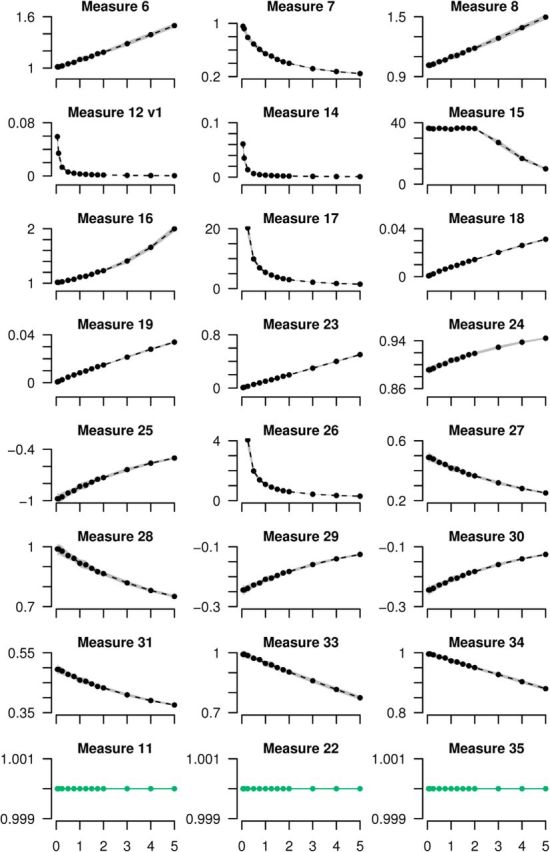
Twenty-one measures are rejected because they are dependent on firing rate (lack property N2). All measures which showed rate-dependence when tested on the autocorrelation of Poisson spike trains are plotted. Three measures which did not show rate-dependence are also shown in the bottom row for comparison (green). One Poisson spike train was simulated for 300 s for varying rates (0.05–5 Hz) and the measures were calculated comparing this spike train to itself. The mean of 10 repeats are plotted and ±1 SD is shown by gray shading. The identity of each measure appears in Table 3. Note that the correlation index is not presented here, but in Figure 3 and that measure 12 has two versions; one appears here and the other in Figure 5A; see Materials and Methods for details.

Figure 5.

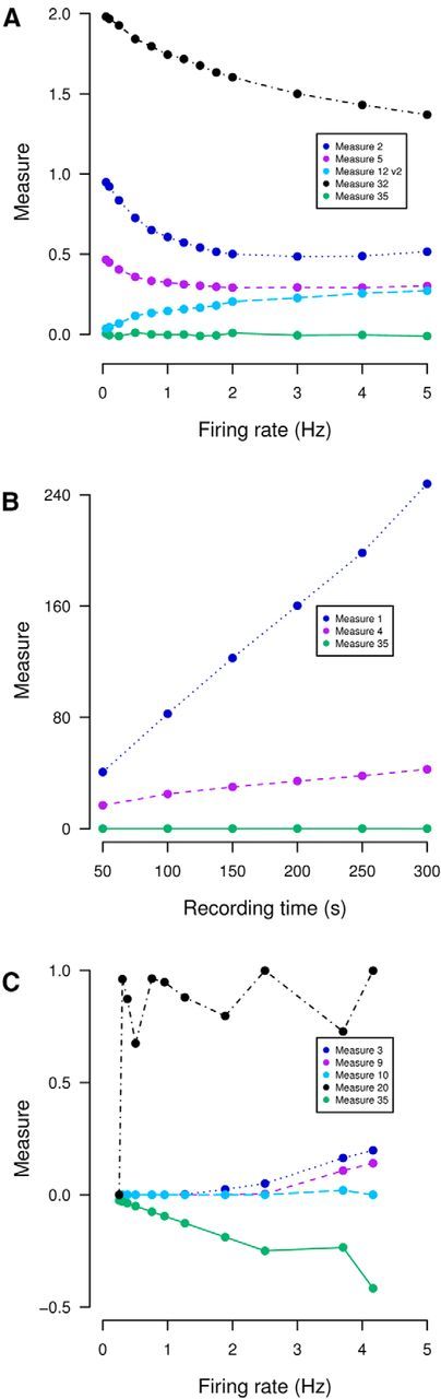
Nine measures are rejected using remaining necessary properties. A, Measures which are dependent on firing rate (lack property N2) where dependency is not obvious from autocorrelation are applied to data generated from the following Poisson spiking model: one train has rate 3 Hz and the other's rate varies (0.1–5 Hz). There are no shared spike times (T = 300 s). The second version of Measure 12 is shown (the first version is in Fig. 4); see Materials and Methods for details. B, Measures which are dependent on recording time (lack property N3) are applied to data generated from the following Poisson spiking model: both neurons fire at rate 1 Hz and 10% of spike times are shared. The recording duration varies from 50 to 300 s and Δt = 0.6 s (higher than usual because for these measures smaller values cause issues with computational precision). C, Measures which cannot distinguish anticorrelation from no correlation (lack property N6) are applied to regular out-of-synchrony spikes of varying rate (0.25–4.2 Hz) generated using an integrate-and-fire model described by Dayan and Abbott, 2001 (their Fig. 5.20). The parameters are as in their figure with the following exceptions: P_max = 0.5, R_mI_e = 18 mV. τ_s varied from 0.05–1.5 s and E_s from 0 mV to −70 mV, T = 3000 s. In all panels, Measure 35 (which possesses the necessary properties) is shown for comparison (green), the mean of 10 repeats are plotted and error bars are omitted for visual clarity.

The remaining 10 measures were tested to ascertain whether they were robust to the amount of data available (property N3) which in practice is proportional to the recording time. Measures should therefore be independent of this (within experimental ranges; minimum 2 min with usual range 20–100 min; Eglen et al., 2014). To test this, two Poisson spike trains with fixed rates and correlations were simulated for different recording times. Two measures showed dependency and so were rejected (Fig. 5B). These measures were a distance measure and a cost function, which are not normalized and so increase as the number of spikes increases.

The eight remaining measures were then tested for the correct range (property N4). They should be equal to +1 for identical spike trains, 0 for no correlation and −1 for strong anti-correlation. All measures were bounded and therefore could be scaled to have the required range provided that they can discriminate between no correlation and anticorrelation (property N6) and so none were rejected at this point.

All eight measures were found to be robust to small variations in Δt (property N5). Of these eight measures, four were rejected because they could not distinguish no correlation from anticorrelation (property N6). The test case on which these measures were removed was regular out-of-synchrony spiking (Fig. 5C). The measures rejected were measures of similarity, rather than correlation, which therefore could not distinguish this firing pattern from independent spike times.

In summary, 31 of 35 measures were rejected in Step 1 as they lacked at least one necessary property. A list of each measure considered and the reason for its rejection can be found in Table 3.

Step 2: selecting one measure based on desirable properties

The four measures possessing all necessary properties were as follows: (1) the spike count correlation (Eggermont, 2010), (2) the Kerschensteiner and Wong (2008) measure, (3) an altered version of the correlation measure from Kruskal et al. (2007), and (4) the spike time tiling coefficient. A brief description of each measure is given in Materials and Methods. Selecting one measure proceeded on the basis of desirable properties (Table 2). These affect either the range of correlations (D1: periods of silence should not count as correlated), the applicability of the measure (D2: spike times should not be assumed to follow a particular distribution), or mean that extra information is required to compare correlations (D3: extra parameters are discouraged).

The spike count correlation calculates the Pearson's correlation coefficient of binned spike counts. We set our bin width to Δt (see Materials and Methods). Because firing rates are sparse, a large proportion of bins have zero spikes in both trains, which counts as correlated. This distorts the values of correlations making results difficult to interpret (Fig. 6A,B). The spike count correlation therefore lacks property D1 but does possess properties D2 and D3. A further limitation is that spikes which are within ±Δt of each other may fall into different bins and these coincidences are missed. It has also been reported that the spike count correlation increases with firing rate (de la Rocha et al., 2007), which lessens its ability to compare correlations fairly. This is not reported here because variation in firing rate was small compared with variation across trials on the time scales considered.

Figure 6.

Detailed examination of the four measures which possess all necessary properties eliminates three on the basis of the desirable properties. A, The spike count correlation with different bin widths (d; see Materials and Methods) is applied to data from the following Poisson burst model which has increasing range of spike offsets within a burst: both neurons have a burst rate of 0.05 Hz, burst centers have 0 s offset, each burst contains eight spikes whose positions are drawn from a uniform distribution of varying width (0.1–4 s) centered on the burst center (T = 3600 s). B, The spike time tiling coefficient (STTC) applied to identical data to that in A. The spike count correlation with d = 1 ms is plotted (black) for comparison. C, The Kerschensteiner and Wong correlation measure with different lengths of the averaging window (w; see Materials and Methods) is applied to data from the following Poisson burst model with increasing number of spikes per burst: both neurons have a burst rate of 0.05 Hz, burst centers have 0 s offset, the number of spikes in each burst is drawn from a Poisson distribution with increasing mean (from 1 to 15). Spike positions are drawn from a uniform distribution of width 2 s centered on the center of the burst (T = 3600 s). D, The Kruskal measure is applied to spike times from the following model: two independent Poisson neurons are simulated each with rate 0.1 Hz. For each spike (in either train) a burst is generated in the other train with 0 s offset of the burst center and one to six spikes whose positions are drawn from a uniform distribution of width 2Δt around the burst center (T = 2000 s, Δt = 0.1 s). The spike time tiling coefficient (green) is plotted in C and D for comparison. For all panels the mean of 10 repeats is plotted, error bars are omitted for visual clarity.

The Kerschensteiner and Wong measure is an altered version of the spike count correlation which replaces the global average firing rate with a local average firing rate (using a sliding window) which prevents periods of silence counting as correlated. Data are binned into bins of width Δt and the sliding window calculates a local average across a fixed number of bins. Although the alteration is effective, this measure possesses desirable properties D1 and D2, it introduces an extra parameter: the length of the sliding window (discouraged by property D3). In order for this measure to be informative, the length of the sliding window must be optimized for the data. If the sliding window is too large compared with the periods of quiescence, then when both trains are quiet, the correlation at that point will be positive. If it is shorter than the burst lengths, then periods where one neuron has a burst and the other does not will count as zero (should count as anticorrelated) because in the silent train both the local average and the individual spike counts will be zero (Eq. 5). Therefore the measure varies qualitatively with this parameter (Fig. 6C), especially on burst-like data. Correlations cannot be fairly compared if this parameter varies, which it is likely to because a poor choice of parameter can lead to uninformative values of correlation.

The altered version of the Kruskal et al. (2007) measure changes the spike count correlation to overcome the fact that coincidences may be missed if they fall in different bins: it smooths spike trains with a boxcar kernel before calculations. This does not possess property D1 as silence is still counted as correlated. It does possess property D2 and D3 (because it is possible to calculate exactly).

The spike time tiling coefficient does not count periods of quiescence as correlated and thus possesses property D1. It does not assume a statistical distribution of spike times and therefore possess property D2. The only free parameter is Δt and it therefore possesses property D3.

Although the Kruskal et al. (2007) measure lacks necessary property D1 which reduces the range of correlations produced, this effect is not as large as for the spike count correlation. We also note that the Kruskal et al. (2007) measure is like a “similarity measure” in the sense that it takes value +1 only if the spike trains are identical whereas the spike time tiling coefficient is equal to +1 for a wider range of firing patterns (those where P_A = P_B = 1) and identical trains can be distinguished from those which are merely highly correlated by letting Δt → 0. Because the Kruskal et al. (2007) measure is close to a similarity measure, relatively low values of correlation can be assigned to highly correlated firing patterns. For instance, consider two spike trains, where if one has a single spike, the other fires several spikes within ±Δt of that spike and vice versa. This is clearly highly correlated (a firing pattern which is indicative of some relationship between the neurons) although the spike trains are not similar so the Kruskal et al. (2007) measure assigns low values of correlation. This value depends on the number of spikes fired when there is one spike in the other train (Fig. 6D) and misrepresents the correlation. The spike time tiling coefficient assigns a correlation value of +1 independent of the number of spikes.

In practice both the Kruskal et al. (2007) and the spike time tiling coefficient were found to be adequate reporters of correlation on experimental data. Because the Kruskal measure lacks property D1 and assigns high correlations only to similar spike trains, the spike time tiling coefficient is able to pick up a larger range of correlated firing patterns and we therefore recommend it to replace the correlation index.

Reanalysis of experimental data using the spike time tiling coefficient

The issues with the correlation index raise questions about the reliability of studies which have used it to draw their conclusions. Because the correlation index is confounded by firing rate, it should not be used to compare correlations in data where rates differ significantly. Firing rates frequently vary across age, phenotype, and presence of pharmacological agonists and so this calls into question the results of many correlation analyses: some conclusions about differences in correlations may be due to the confounding effect of the firing rates, and not the correlations themselves. Because the correlation index has been widely used in the field (we found 43 papers that used it, 29 of which have been published since 2008), we also considered the wider implications of its use. In particular, what conclusions were at risk of changing if the data were to be reanalyzed using the spike time tiling coefficient? Four examples using seven studies in the developing retina are presented to demonstrate the use of the spike time tiling coefficient in place of the correlation index. For this work, we used the freely available retinal wave data from the CARMEN portal (Eglen et al., 2014; https://portal.carmen.org.uk/).

Example 1: connexin isoforms

Reanalysis of existing recordings of spontaneous retinal waves using the spike time tiling coefficient in place of the correlation index can show significant differences. As an example, we reanalyzed MEA recordings from Blankenship et al. (2011), which compared the statistical properties of wild-type spontaneous retinal activity to those from mutant mice lacking either one or two connexin isoforms (Cx45 and Cx36/Cx45). This study reported that the two mutants exhibit substantially higher firing rates compared with wild-type (Fig. 7A) and when the correlation indices are calculated pairwise and plotted against electrode separation (the standard analysis) the size of the correlation depends inversely on the mean firing rate (Fig. 7B). That is, wild-type has both the lowest firing rate and the highest correlation and Cx36/Cx45dko has the highest firing rate and the lowest correlation. From the raster plots (Fig. 7A) all phenotypes exhibit some correlated firing and the differences in correlation patterns are not as large as the differences in firing rate.

Figure 7.

Evaluating correlations in retinal waves recorded from connexin mutant mice shows that the spike time tiling coefficient can significantly alter conclusions. A, Raster plots of 10 spike trains over a 10 min interval, recorded from retinas isolated from P12 wild-type mouse and two mutant mice (lacking either one or two connexin isoforms- Cx45 and Cx36/Cx45), P11 Cx45ko and P10 Cx36/Cx45dko. Data are from Blankenship et al. (2011) and raster plots follow the presentation of their Figure 2A. The mean firing rate and number of animals (n) from each genotype is recorded in the legend. B, Pairwise correlation index as a function of intercellular distance for each genotype. Data points are medians over all recordings and error bars indicate the interquartile range (IQR). Inset, The same data normalized (multiplicatively) by genotype so that the correlation indices are identical at zero distance, following Figure 2B in the original publication. C, Same as B, using the STTC in place of the correlation index. Compare with both B and B, inset. In both B and C, Δt = 100 ms as in the original publication. The distances at which correlations are measured are the discrete set of separations possible on the MEA grid.

When the data are reanalyzed using the spike time tiling coefficient, the results are strikingly different (Fig. 7C): wild-type and Cx45ko have highly similar correlation values and the difference between correlations in wild-type and Cx36/Cx45dko are much smaller. Although correlations are difficult to judge from the raster plots, those of wild-type and Cx45ko have several correlational features in common: they both show waves and also some correlated spiking outside of waves. Waves cannot clearly be seen in the raster plot of Cx36/45dko, although there is correlated firing. The relative correlations of these phenotypes measured using the correlation index reflect the differences in firing rate, whereas, when measured using the spike time tiling coefficient, they reflect differences in correlational structure (Fig. 7A).

In the original publication, the authors noted that the correlation values for Cx36/Cx45dko were so low that it was difficult to deduce anything about its distance dependence relative to the other phenotypes. To make this comparison they (multiplicatively) normalized the correlation indices so that all phenotypes had the same value (the wild-type value) at zero distance. From this they deduced that the distance dependence of wild-type and Cx45ko were very similar and also that the correlations of Cx36/Cx45dko had a weaker distance dependence than the other two phenotypes. This result is immediately apparent using the spike time tiling coefficient, without the need to normalize: wild-type and Cx45ko have very similar values at all distances and Cx36/Cx45dko has weaker distance dependence. This phenotype has less correlation than the other two at smaller distances and more correlation at greater distances (≥400 μm). This is not apparent using the correlation index; the spike time tiling coefficient thus provides a more informative comparison of the correlations.

Example 2: developmental changes in correlation

A key result used to support the hypothesis that correlated activity plays a role in map formation is that correlations in spontaneous retinal activity decrease with age both in ferret (Wong et al., 1993) and mouse (Demas et al., 2003). These studies reported different variation in firing rates with age: firing rates decrease with age in ferret, but increase with age in mouse (confirmed by Maccione et al., 2014). Because neurons with high firing rates have down-weighted correlation indices, it is possible that this result is due to the confounding effect of the increasing firing rates in mouse. This is unlikely to be the case in ferret where firing rates decrease. Reanalysis with the spike time tiling coefficient confirmed that in both cases, correlations do decrease with age and so this conclusion stands (Fig. 8).

Figure 8.

Reanalysis using the spike time tiling coefficient supports the conclusion that correlations in spontaneous activity in the developing ferret and mouse retina decreases with age. A, The correlation index is calculated pairwise and shown as a function of electrode separation for spontaneous retinal activity in developing ferret for four different ages (data from Wong et al., 1993). The distances at which correlations are measured were binned (bin width 20 μm) due to high density. B, Same as A using the STTC in place of the correlation index. C, The correlation index is calculated pairwise and shown as a function of electrode separation for spontaneous retinal activity in developing mouse for four different ages (data from Demas et al., 2003). The distances at which correlations are measured are the discrete set of separations possible on the MEA grid. D, Same as C using the STTC. In all panels, median values are plotted and IQRs are only shown at the smallest separation distance. Other IQRs are omitted for visual clarity. Mean firing rates and number of animals (n) for each age are recorded in the legend.

Example 3: β2 genotypes

A key group of genetically modified mice which provide (somewhat controversial) evidence that correlations are key to map formation is the β2(KO) mutants (animals lacking the β2 subunit of the nicotinic acetylcholine receptor) which form a defective retinotopic map. This mutant was initially thought to have uncorrelated activity (McLaughlin et al., 2003), but it was later shown that retinal waves exist (Sun et al., 2008; Stafford et al., 2009). The β2(KO) mice have slightly higher firing rates and weaker distance-dependence of correlations than wild-type (typically at short distances these mutants have lower correlation than wild-type, but they have higher correlation at large distances). Reanalysis of data from Sun et al. (2008) and Stafford et al. (2009) using the spike time tiling coefficient confirms reported results (Fig. 9).

Figure 9.

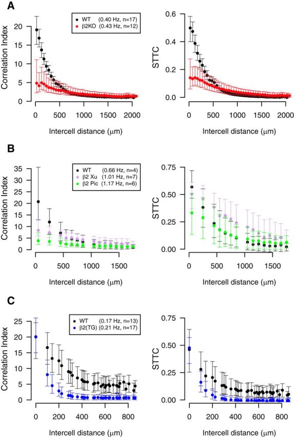
Reanalysis of experimental data using the spike time tiling coefficient supports the conclusions that the β2(KO) and β2(TG) mouse phenotypes show lower correlations in spontaneous retinal activity than those of wild-type. A, The correlation index (left) or STTC (right) is plotted pairwise against electrode separation for recordings of spontaneous retinal activity for P6 wild-type and β2(KO) phenotypes (data from Stafford et al., 2009). B, The correlation index (left) or spike time tiling coefficient (right) is plotted pairwise against electrode separation for recordings of spontaneous retinal activity for P5 wild-type and two β2(KO) phenotypes: Xu and Picciotto (Pic) (data from Sun et al., 2008). C, The correlation index (left) or spike time tiling coefficient (right) is plotted pairwise against electrode separation for recordings of spontaneous retinal activity for P4 wild-type and β2(TG) phenotypes (data from Xu et al., 2011). In all panels, Δt = 100 ms, as in original publications, medians are plotted and the error bars show the IQR. Mean firing rates and number of animals (n) for each phenotype are recorded in the legend. All recordings at 37°C. The distances at which correlations are measured are the discrete set of separations possible on the MEA grid.

Although the conclusion stands, reanalysis of the data from Sun et al. (2008) shows differences from the original analysis (Fig. 9B): the correlation indices are noticeably confounded by the firing rates which differ across the genotypes. Reanalysis using the spike time tiling coefficient shows that the differences in correlation between phenotypes are smaller than previously reported; all three phenotypes now show significant correlation at short distances. The order of phenotypes by correlation at short distance [wild-type is highest, β2(KO) (Picciotto) is lowest] is preserved as is the order by distance dependence [wild-type is strongest, β2(KO) (Picciotto) is weakest].

Reanalysis of recordings of the β2(TG) mouse (Xu et al., 2011) confirm that this phenotype shows weaker correlations than that of wild-type (Fig. 9).

Example 4: age-related changes in β2(KO)

Retinal waves of β2(KO) mutants at different ages (P4–P7 and wild-type P5–P6) were recorded by Kirkby and Feller (2013) as controls in their study of intrinsically photosensitive retinal ganglion cells. Sample raster plots for P4 β2(KO) and P5 wild-type are shown in Figure 10A. Firing rates of the β2(KO) mutants increase (Fig. 10, see legend) and their correlation indices decrease (Fig. 10B) with age. In addition, P4 and P5 β2(KO) are extremely and erratically correlated, whereas P6–P7 β2(KO) and wild-type show typical correlations and distance dependence. One might, therefore, conclude that the recordings of P4–P5 β2(KO) show highly correlated and extremely unusual firing patterns. However, this is not borne out by inspection of the raster plots (Fig. 10A); the firing patterns of the P4 β2(KO) mutant are not too dissimilar to those of wild-type, albeit occurring at a much lower rate. We note that the mean firing rates β2(KO) P4–P5 are low compared with other ages (and wild-type) and so this behavior is likely to be due to the confounding effect of the firing rates. Reanalysis of these data using the spike time tiling coefficient confirms this (Fig. 10C): all correlations and distance dependencies are now within typical ranges. These two phenotypes (β2(KO) P4–P5) still show more variability in their distance dependencies, but we note that this is likely to be due to the small number of recordings, and that this variability is much less than that seen using the correlation index.

Figure 10.

Reanalysis of age related changes in β2(KO) mutants shows that the spike time tiling coefficient is able to more accurately quantify correlations which the correlation index ascribes as extremely correlated. A, Raster plots of 10 spike trains over a 10 min interval, recorded from retinas isolated from P5 wild-type mouse and P4 β2(KO) mouse. All data are controls from Kirkby and Feller (2013). B, Pairwise correlation index as a function of intercellular distance for P5 wild-type mouse and β2(KO) mouse of different ages (P4–P7). C, Same as B but using STTC. The mean firing rate and number of animals (n) from each genotype is recorded in the legend. Data points are medians over all recordings and error bars indicate the IQR. For visual clarity, IQRs are only shown at the smallest separation distance. The distances at which correlations are measured are the discrete set of separations possible on the MEA grid. Δt = 100 ms, as in original publication and recordings were performed at 33–35°C.

This reanalysis alters the conclusion that correlations in β2(KO) genotypes decrease with age (in P4–P7), which is caused by the confounding effect of increasing firing rates. Analysis with the spike time tiling coefficient shows that they tend to increase with age (the order of correlations from lowest to highest is P5, P4, P6, P7).

Variation of window of synchrony Δt can reveal timescales of correlation

The coincidence window Δt is a free parameter which should be fixed to compare correlations. It can also be used to find time scales of correlation in a dataset. Figure 11 shows how varying Δt changes the spike time tiling coefficient (for the data from Example 3). Useful timescales can be found by considering local maxima and minima and the gradient of spike time tiling coefficient (note that the limit of the spike time tiling coefficient as Δt → T is +1). For instance in all panels of Figure 11 there is a clear change in gradient at around 0.5–1 s which could indicate a timescale of correlation. In Figure 11A,B, the wild-type gradient is largest between 0.01 and 0.05 s as is β2(TG) in Figure 11C, which could also indicate a useful scale. Differences in correlational time scales between phenotypes are also apparent, for instance in Figure 11C, wild-type spikes are less correlated than those of β2(TG) on timescales of Δt ≤ 0.1 s and more correlated than β2(TG) on larger timescales (note, however, significant overlap of error bars).

Figure 11.

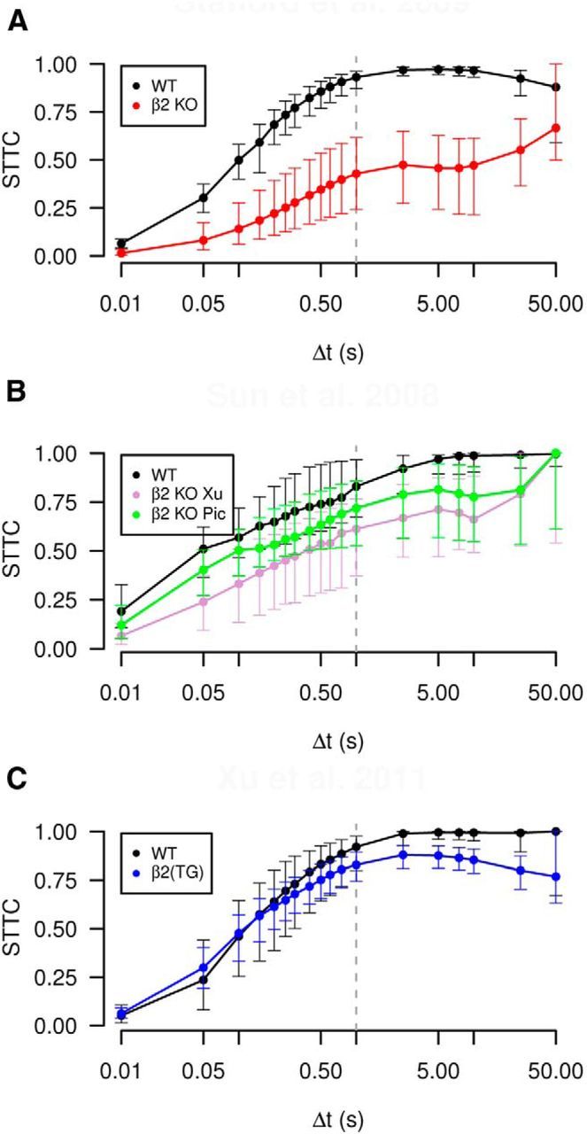
Varying the window of synchrony Δt can be informative about correlational timescales inherent in data. A, The STTC of spike trains from Stafford et al. (2009) was calculated pairwise (as in Fig. 9B) and the median value at the smallest electrode separation is plotted for varying Δt. Error bars show the IQR. The genotypes shown are P6 wild-type and β2(KO). B, Same as A, but data from Sun et al., 2008; Fig. 9D). The genotypes shown are P5 wild-type and two β2(KO) phenotypes: Xu and Picciotto (Pic). C, Same as A, but data from Xu et al., 2011 (Fig. 9F). The genotypes shown are P4 wild-type and β2(TG) mouse. Vertical lines at Δt = 1 s indicate separation between region with strong Δt dependency (Δt ≤ 1) and weaker dependency (note x-axis has a log-scale and that the limit of the spike time tiling coefficient as Δt tends to infinity is one).

Discussion

We have described the need to correctly quantify neuronal correlations and considered a popular measure, the correlation index. We have shown that it is confounded by firing rate and is unbounded above which means it cannot fairly compare correlations when firing rates differ significantly. We aimed to find a measure which could be used as a replacement for the correlation index and which could fairly compare correlations. We listed necessary and desirable properties that such a measure needs and found 33 other existing measures of correlation. Because no measure obviously possessed all listed properties, we proposed a novel measure of correlation; the spike time tiling coefficient. We blindly tested all measures for the properties using synthetic and experimental data. We reiterate that no existing measure was designed to replace the correlation index so the exclusion of a measure is no reflection of its usefulness. Four measures possessed all the required properties and the spike time tiling coefficient was chosen as the most appropriate replacement based on the desirable properties. To demonstrate its use we reanalyzed data from seven studies and showed that it can significantly alter conclusions.

The form and use of the spike time tiling coefficient

Both the correlation index and the spike time tiling coefficient use a small time window to identify spike pairs which are indicative of an overall correlation between the spike trains. We quantify correlations that are functionally significant, which are typically those which can affect synaptic change. In spontaneous retinal waves, correlated activity is thought to contribute to map formation by helping neighboring neurons wire to common targets via a Hebbian mechanism (Demas et al., 2003). This process has a critical time window: studies of spike-time-dependent-plasticity (Zhang et al., 1998) provide a means to estimate its width, which is age- and species-dependent, ∼50–500 ms (Lee et al., 2002). More recently, other rules, such as burst-time-dependent-plasticity, suggest longer windows (Butts et al., 2007).

The time window, Δt, can take any value of interest; often that value is dictated by the phenomenon being investigated. For instance, in spontaneous retinal activity, Δt is dictated by spike-time-dependent-plasticity and in cortical circuits, local oscillatory events could be used to find a Δt of interest as they are reporters of synchrony (Harris et al., 2003). If there is no prior Δt of interest, its value could be varied to show timescales of correlations (Fig. 11). If varying Δt is infeasible, an approximate value of interest could be generated by inspection of cross-correlograms.

The spike time tiling coefficient assumes stationary spiking patterns. Correlations calculated from highly nonstationary data may be misleading as network states greatly influence firing patterns in, e.g., hippocampal firing, so the average value of correlation may not accurately represent the data. Changes in correlation over a nonstationary recording can be identified using the spike time tiling coefficient by calculating it within a sliding window to get a temporally varying correlation. This window must be large enough to capture representative behavior and so if it is required to capture changes in correlation on a very small timescale, a measure which incorporates some form of localized measurement (Kerschensteiner and Wong, 2008) may be preferable.

We have used the word “correlation” throughout but noted that the terminology varies. Few of the measures measure correlation in the statistical sense (the degree to which measurements on the same group of elements tend to vary together). Neither the correlation index nor the spike time tiling coefficient are correlations under this definition. The only “true” correlation is the spike count correlation coefficient (and the altered versions).

We suggest that the correct terminology for what we measure is “affinity” in the biological sense; meaning a relationship or resemblance in structure that suggests a common origin or purpose. We measure a relationship between spike times that may indicate that neurons are involved in the same process. In spontaneous retinal activity, we measure the propensity of two neurons to fire close in time to each other in such a way that it can affect their wiring onto a common target.

Pairwise measures of correlation will only capture a subset of the full correlational relationships in a neuronal population. Population dynamics are less noisy than pairwise dynamics and may encode critical information. Methods exist to study higher-order correlations (Nakahara and Amari, 2002; Walters et al., 2008) and investigating population dynamics is a common approach (Okun et al., 2012). We have focused on pairwise correlations, partly due to its popularity and the large literature concerning its quantification but also as evidence suggests that pairwise interactions can account for much of the observed higher-order interactions (Shlens et al., 2006; Schneidman et al., 2006).

The spike time tiling coefficient in the reanalysis of data and cross-study comparisons

We have reanalyzed the results of seven studies using the spike time tiling coefficient instead of the correlation index. This has shown that sometimes the correlation index reflects differences in firing rate more than differences in correlation and so the spike time tiling coefficient can change the conclusions of studies. For example, our reanalysis of the data from Blankenship et al. (2011) significantly changes the conclusions about the relative correlations in spontaneous retinal activity of connexin knock-out mutants.

The popularity of the correlation index means that many studies have drawn conclusions on the basis of a problematic measure. Studies where firing rates differ significantly and the order of phenotypes by correlation is the reverse of the order by firing rate are likely to change. However, of these, we have shown that two important conclusions made using the correlation index still stand when reanalyzed with the spike time tiling coefficient. These are the age-dependent changes in wild-type correlations in mouse and ferret (Fig. 8) and also relative correlations of wild-type and β2(KO) mouse mutants (Fig. 9).

Although the reanalysis of data from β2 mutants broadly confirms the conclusions of the original studies, the correlations of the two β2(KO) mutants from Sun et al. (2008) show stronger distance-dependence and values closer to wild-type than was evident using the correlation index (Fig. 9B). Both mutants have relatively high firing rates (Fig. 9, see legend) so their correlation indices are down-weighted, making the distance dependence appear weaker.

The β2(KO) mutant line used in Stafford et al. (2009) is the same as the Xu knock-out line used in Sun et al. (2008) with ages P6 and P5, respectively. We note variation between studies of the size and distance dependence of these correlations. Some of the variation between reported correlations may be due to different bath solutions (Stafford et al., 2009), or possibly to age-related differences. However, we also note large cross-study variation in the wild-type control (P4, Xu et al., 2011; P5, Sun et al., 2008; and P6, Stafford et al., 2009). Given that they are similar ages, we would expect control firing rates and correlations to be reasonably similar (Wong et al., 1993); however, both the firing rates and maximal correlation values vary significantly (Fig. 9). Variation between studies for the controls is large so the differences observed in β2(KO) between studies are not surprising given this and the use of different bath solutions.

One conclusion about the correlations in β2(KO) which changed when reanalyzed using the spike time tiling coefficient is that correlations tend to increase during P4–P7, rather than decrease (Fig. 10). This case provides a good example of how the correlation index can assign extreme values to data which is not atypical but which has low firing rates. These data are typically excluded as outliers: many studies filter neurons for extremely low or high firing rates before calculating correlations (Maccione et al., 2014). However, reanalysis using the spike time tiling coefficient shows that this is not necessary: meaningful conclusions about correlations can still be obtained from these data.

Conclusions

Here, we have used spontaneous retinal activity as a case study. Because quantifying correlations in spike times is of wider interest, we expect the spike time tiling coefficient to have applications to measuring correlations in other systems, such as hippocampal cultures (Godfrey and Eglen, 2009), multisensory integration (Parise et al., 2013), or motor control (Lee and Lisberger, 2013). With regards to our case study, we hope that its use will help clarify the exact role of correlations in map formation.

Notes

Supplemental material for this article is available at https://github.com/CCutts/Detecting_pairwise_correlations_in_spike_trains. This project repository contains freely available code relating to this project and links to a freely available R package in which the spike time tiling coefficient is implemented. It also links to a document containing the derivation of Equations 2 and 3 and the mathematical details of the choice of normalization for the spike time tiling coefficient. This material has not been peer reviewed.

References

- Ackman JB, Burbridge TJ, Crair MC. Retinal waves coordinate patterned activity throughout the developing visual system. Nature. 2012;490:219–225. doi: 10.1038/nature11529. [DOI] [PMC free article] [PubMed] [Google Scholar]
- Blankenship AG, Hamby AM, Firl A, Vyas S, Maxeiner S, Willecke K, Feller MB. The role of neuronal connexins 36 and 45 in shaping spontaneous firing patterns in the developing retina. J Neurosci. 2011;31:9998–10008. doi: 10.1523/JNEUROSCI.5640-10.2011. [DOI] [PMC free article] [PubMed] [Google Scholar]
- Butts DA, Kanold PO, Shatz CJ. A burst-based Hebbian learning rule at retinogeniculate synapses links retinal waves to activity-dependent refinement. PLoS Biol. 2007;5:e61. doi: 10.1371/journal.pbio.0050061. [DOI] [PMC free article] [PubMed] [Google Scholar]
- Chiappalone M, Bove M, Vato A, Tedesco M, Martinoia S. Dissociated cortical networks show spontaneously correlated activity patterns during in vitro development. Brain Res. 2006;1093:41–53. doi: 10.1016/j.brainres.2006.03.049. [DOI] [PubMed] [Google Scholar]
- Cressie NAC. Statistics for Spatial Data. New York: Wiley; 1993. [Google Scholar]
- Dayan P, Abbott LF. Theoretical neuroscience: computational and mathematical modelling of neural systems. Cambridge: MIT; 2001. [Google Scholar]
- de la Rocha J, Doiron B, Shea-Brown E, Josić K, Reyes A. Correlation between neural spike trains increases with firing rate. Nature. 2007;448:802–806. doi: 10.1038/nature06028. [DOI] [PubMed] [Google Scholar]
- Dehorter N, Vinay L, Hammond C, Ben-Ari Y. Timing of developmental sequences in different brain structures: physiological and pathological implications. Eur J Neurosci. 2012;35:1846–1856. doi: 10.1111/j.1460-9568.2012.08152.x. [DOI] [PubMed] [Google Scholar]
- Demas J, Eglen SJ, Wong RO. Developmental loss of synchronous spontaneous activity in the mouse retina is independent of visual experience. J Neurosci. 2003;23:2851–2860. doi: 10.1523/JNEUROSCI.23-07-02851.2003. [DOI] [PMC free article] [PubMed] [Google Scholar]
- Demas J, Sagdullaev BT, Green E, Jaubert-Miazza L, McCall MA, Gregg RG, Wong RO, Guido W. Failure to maintain eye-specific segregation in nob, a mutant with abnormally patterned retinal activity. Neuron. 2006;50:247–259. doi: 10.1016/j.neuron.2006.03.033. [DOI] [PubMed] [Google Scholar]
- Eggermont JJ. Pair-correlation in the time and frequency domain. In: Grun S, Rotter S, editors. Analysis of parallel spike trains. New York: Springer; 2010. pp. 77–102. [Google Scholar]
- Eglen SJ, Weeks M, Jessop M, Simonotto J, Jackson T, Sernagor E. A data repository and analysis framework for spontaneous neural activity recordings in developing retina. GigaScience. 2014;3:3. doi: 10.1186/2047-217X-3-3. [DOI] [PMC free article] [PubMed] [Google Scholar]
- Eytan D, Minerbi A, Ziv N, Marom S. Dopamine induced dispersion of correlations between action potentials in networks of cortical neurons. J Neurophysiol. 2004;92:1817–1824. doi: 10.1152/jn.00202.2004. [DOI] [PubMed] [Google Scholar]
- Feller MB. Retinal waves are likely to instruct the formation of eye-specific retinogeniculate projections. Neural Dev. 2009;4:24. doi: 10.1186/1749-8104-4-24. [DOI] [PMC free article] [PubMed] [Google Scholar]
- Godfrey KB, Eglen SJ. Theoretical models of spontaneous activity generation and propagation in the developing retina. Mol Biosyst. 2009;5:1527–1535. doi: 10.1039/b907213f. [DOI] [PubMed] [Google Scholar]
- Grün S, Diesmann M, Aertsen A. Unitary events in multiple single-neuron spiking activity: I. Detection and significance. Neural Comput. 2002;14:43–80. doi: 10.1162/089976602753284455. [DOI] [PubMed] [Google Scholar]
- Harris KD, Csicsvari J, Hirase H, Dragoi G, Buzsáki G. Organisation of cell assemblies in the hippocampus. Nature. 2003;424:552–556. doi: 10.1038/nature01834. [DOI] [PubMed] [Google Scholar]
- Hunter JD, Milton JG. Amplitude and frequency dependence of spike timing: implications for dynamic regulation. J Neurophysiol. 2003;90:387–394. doi: 10.1152/jn.00074.2003. [DOI] [PubMed] [Google Scholar]
- Isham V. Marked point processes and their correlations. In: Droesbeke F, editor. Spatial processes and spatial time series analysis. Brussels: Publications des Facultes Universitaires Saint-Louis; 1985. pp. 63–75. [Google Scholar]
- Jimbo Y, Tateno T, Robinson HP. Simultaneous induction of pathway-specific potentiation and depression in networks of cortical neurons. Biophys J. 1999;76:670–678. doi: 10.1016/S0006-3495(99)77234-6. [DOI] [PMC free article] [PubMed] [Google Scholar]
- Joris PX, Louage DH, Cardoen L, van der Heijden M. Correlation index: a new metric to quantify temporal coding. Hear Res. 2006;216:19–30. doi: 10.1016/j.heares.2006.03.010. [DOI] [PubMed] [Google Scholar]
- Kerschensteiner D, Wong RO. A precisely timed asynchronous pattern of ON and OFF retinal ganglion cell activity during propagation of retinal waves. Neuron. 2008;58:851–858. doi: 10.1016/j.neuron.2008.04.025. [DOI] [PMC free article] [PubMed] [Google Scholar]
- Kirkby LA, Feller MB. Intrinsically photosensitive ganglion cells contribute to plasticity in retinal wave circuits. Proc Natl Acad Sci U‖SA. 2013;110:12090–12095. doi: 10.1073/pnas.1222150110. [DOI] [PMC free article] [PubMed] [Google Scholar]
- Kirkby LA, Sack GS, Firl A, Feller MB. A role for correlated spontaneous activity in the assembly of neural circuits. Neuron. 2013;80:1129–1144. doi: 10.1016/j.neuron.2013.10.030. [DOI] [PMC free article] [PubMed] [Google Scholar]
- Kreuz T, Haas JS, Morelli A, Abarbanel HD, Politi A. Measuring spike train synchrony. J Neurosci Methods. 2007a;165:151–161. doi: 10.1016/j.jneumeth.2007.05.031. [DOI] [PubMed] [Google Scholar]
- Kreuz T, Mormann F, Andrzejak RG, Kraskov A, Lehnertz K, Grassberger P. Measuring synchronisation in coupled model systems: a comparison of different approaches. Phys D. 2007b;225:29–42. doi: 10.1016/j.physd.2006.09.039. [DOI] [Google Scholar]
- Kreuz T, Chicharro D, Houghton C, Andrzejak RG, Mormann F. Monitoring spike train synchrony. J Neurophysiol. 2013;109:1457–1472. doi: 10.1152/jn.00873.2012. [DOI] [PubMed] [Google Scholar]
- Kruskal PB, Stanis JJ, McNaughton BL, Thomas PJ. A binless correlation measure reduces the variability of memory reactivation estimates. Stat Med. 2007;26:3997–4008. doi: 10.1002/sim.2946. [DOI] [PubMed] [Google Scholar]
- Lee CW, Eglen SJ, Wong RO. Segregation of ON and OFF retinogeniculate connectivity directed by patterned spontaneous activity. J Neurophysiol. 2002;88:2311–2321. doi: 10.1152/jn.00372.2002. [DOI] [PubMed] [Google Scholar]
- Lee J, Lisberger SG. Gamma synchrony predicts neuron-neuron correlations and correlations with motor behaviour in extrastriate visual area MT. J Neurosci. 2013;33:19677–19688. doi: 10.1523/JNEUROSCI.3478-13.2013. [DOI] [PMC free article] [PubMed] [Google Scholar]
- Li W. Mutual information functions versus correlation functions. J Stat Phys. 1990;60:823–837. doi: 10.1007/BF01025996. [DOI] [Google Scholar]
- Maccione A, Hennig MH, Gandolfo M, Muthmann O, van Coppenhagen J, Eglen SJ, Berdondini L, Sernagor E. Following the ontogeny of retinal waves: pan-retinal recordings of population dynamics in the neonatal mouse. J Physiol. 2014;592:1545–1563. doi: 10.1113/jphysiol.2013.262840. [DOI] [PMC free article] [PubMed] [Google Scholar]
- Macke JH, Berens P, Ecker AS, Tolias AS, Bethge M. Generating spike trains with specified correlation coefficients. Neural Comput. 2009;21:397–423. doi: 10.1162/neco.2008.02-08-713. [DOI] [PubMed] [Google Scholar]
- MacLaren EJ, Charlesworth P, Coba MP, Grant SG. Knockdown of mental disorder susceptibility genes disrupts neuronal network physiology in vitro. Mol Cell Neurosci. 2011;47:93–99. doi: 10.1016/j.mcn.2010.12.014. [DOI] [PMC free article] [PubMed] [Google Scholar]
- McLaughlin T, Torborg CL, Feller MB, O'Leary DD. Retinotopic map refinement requires spontaneous retinal waves during a brief critical period of development. Neuron. 2003;40:1147–1160. doi: 10.1016/S0896-6273(03)00790-6. [DOI] [PubMed] [Google Scholar]
- Nakahara H, Amari S. Information-geometric measure for neural spikes. Neural Comput. 2002;14:2269–2316. doi: 10.1162/08997660260293238. [DOI] [PubMed] [Google Scholar]
- Okun M, Yger P, Marguet SL, Gerard-Mercier F, Benucci A, Katzner S, Busse L, Carandini M, Harris KD. Population rate dynamics and multineuron firing patterns in sensory cortex. J Neurosci. 2012;32:17108–17119. doi: 10.1523/JNEUROSCI.1831-12.2012. [DOI] [PMC free article] [PubMed] [Google Scholar]
- Parise CV, Harrar V, Ernst MO, Spence C. Cross-correlation between auditory and visual signals promotes multisensory integration. Multisens Res. 2013;26:307–316. doi: 10.1163/22134808-00002417. [DOI] [PubMed] [Google Scholar]
- Pasquale V, Massobrio P, Bologna LL, Chiappalone M, Martinoia S. Self-organization and neuronal avalanches in networks of dissociated cortical neurons. Neuroscience. 2008;153:1354–1369. doi: 10.1016/j.neuroscience.2008.03.050. [DOI] [PubMed] [Google Scholar]
- Personius KE, Balice-Gordon RJ. Loss of correlated motor neuron activity during synaptic competition at developing neuromuscular synapses. Neuron. 2001;31:395–408. doi: 10.1016/S0896-6273(01)00369-5. [DOI] [PubMed] [Google Scholar]
- Personius KE, Chang Q, Mentis GZ, O'Donovan MJ, Balice-Gordon RJ. Reduced gap junctional coupling leads to uncorrelated motor neuron firing and precocious neuromuscular synapse elimination. Proc Natl Acad Sci U S A. 2007;104:11808–11813. doi: 10.1073/pnas.0703357104. [DOI] [PMC free article] [PubMed] [Google Scholar]
- Ripley BD. The second-order analysis of stationary point processes. J Appl Prob. 1976;13:255–266. doi: 10.2307/3212829. [DOI] [Google Scholar]
- Schlather M, Ribeiro PJ, Diggle PJ. Detecting dependence between marks and locations of marked point processes. J R Stat Soc B. 2004;66:79–93. doi: 10.1046/j.1369-7412.2003.05343.x. [DOI] [Google Scholar]
- Shlens J, Field GD, Gauthier JL, Grivich MI, Petrusca D, Sher A, Litke AM, Chichilnisky EJ. The structure of multi-neuron firing patterns in primate retina. J Neurosci. 2006;26:8254–8266. doi: 10.1523/JNEUROSCI.1282-06.2006. [DOI] [PMC free article] [PubMed] [Google Scholar]
- Schneidman E, Berry MJ, 2nd, Segev R, Bialek W. Weak pairwise correlations imply strongly correlated network states in a neural correlation. Nature. 2006;440:1007–1012. doi: 10.1038/nature04701. [DOI] [PMC free article] [PubMed] [Google Scholar]
- Schreiber S, Fellous JM, Whitmer D, Tiesinga P, Sejnowski TJ. A new correlation-based measure of spike timing reliability. Neurocomputing. 2003;52:925–931. doi: 10.1016/S0925-2312(02)00838-X. [DOI] [PMC free article] [PubMed] [Google Scholar]
- Shi X, Lu Q. Burst synchronization of electrically and chemically coupled map-based neurons. Phys A. 2009;388:2410–2419. doi: 10.1016/j.physa.2009.03.008. [DOI] [Google Scholar]
- Simpson EH. Measurement of diversity. Nature. 1949;163:688. doi: 10.1038/163688a0. [DOI] [Google Scholar]
- Stafford BK, Sher A, Litke AM, Feldheim DA. Spatial-temporal patterns of retinal waves underlying activity-dependent refinement of retinofugal projections. Neuron. 2009;64:200–212. doi: 10.1016/j.neuron.2009.09.021. [DOI] [PMC free article] [PubMed] [Google Scholar]
- Stoyan D. Correlations of the marks of marked point processes: statistical inference and simple models. Elektron. Informationsverarbeitung und Kybernetik. 1984;20:285–294. [Google Scholar]
- Stoyan D, Stoyan H. Fractals, random shapes and point fields. Chichester: Wiley; 1994. [Google Scholar]
- Sun C, Warland DK, Ballesteros JM, van der List D, Chalupa LM. Retinal waves in mice lacking the beta2 subunit of the nicotinic acetylcholine receptor. Proc Natl Acad Sci U S A. 2008;105:13638–13643. doi: 10.1073/pnas.0807178105. [DOI] [PMC free article] [PubMed] [Google Scholar]
- van Rossum MC. A novel spike distance. Neural Comput. 2001;13:751–763. doi: 10.1162/089976601300014321. [DOI] [PubMed] [Google Scholar]
- Victor JD, Purpura K. Metric-space analysis of spike trains: theory, algorithms and application. Network. 1997;8:127–164. doi: 10.1088/0954-898X/8/2/003. [DOI] [Google Scholar]
- Walters E, Segonds-Pichon A, Nicol AU. The correlation determinant in tests for synchronization in neuronal spike data. J Neurosci Methods. 2008;172:60–66. doi: 10.1016/j.jneumeth.2008.04.003. [DOI] [PubMed] [Google Scholar]
- Wong RO. Retinal waves and visual system development. Annu Rev Neurosci. 1999;22:29–47. doi: 10.1146/annurev.neuro.22.1.29. [DOI] [PubMed] [Google Scholar]
- Wong RO, Meister M, Shatz CJ. Transient period of correlated bursting activity during development of the mammalian retina. Neuron. 1993;11:923–938. doi: 10.1016/0896-6273(93)90122-8. [DOI] [PubMed] [Google Scholar]
- Xu HP, Furman M, Mineur YS, Chen H, King SL, Zenisek D, Zhou ZJ, Butts DA, Tian N, Picciotto MR, Crair MC. An instructive role for patterened spontaneous retinal activity in mouse visual map development. Neuron. 2011;70:1115–1127. doi: 10.1016/j.neuron.2011.04.028. [DOI] [PMC free article] [PubMed] [Google Scholar]
- Zhang LI, Tao HW, Holt CE, Harris WA, Poo M. A critical window for cooperation and competition among developing retinotectal synapses. Nature. 1998;395:37–44. doi: 10.1038/25665. [DOI] [PubMed] [Google Scholar]