The Use of Experimental Structures to Model Protein Dynamics

Summary

The number of solved protein structures submitted in the Protein Data Bank (PDB) has increased dramatically in recent years. For some specific proteins, this number is very high – for example, there are over 550 solved structures for HIV-1 protease, one protein that is essential for the life cycle of human immunodeficiency virus (HIV) which causes acquired immunodeficiency syndrome (AIDS) in humans. The large number of structures for the same protein and its variants include a sample of different conformational states of the protein. A rich set of structures solved experimentally for the same protein has information buried within the dataset that can explain the functional dynamics and structural mechanism of the protein. To extract the dynamics information and functional mechanism from the experimental structures, this chapter focuses on two methods – Principal Component Analysis (PCA) and Elastic Network Models (ENM). PCA is a widely used statistical dimensionality reduction technique to classify and visualize high-dimensional data. On the other hand, ENMs are well-established simple biophysical method for modeling the functionally important global motions of proteins. This chapter covers the basics of these two. Moreover, an improved ENM version that utilizes the variations found within a given set of structures for a protein is described. As a practical example, we have extracted the functional dynamics and mechanism of HIV-1 protease dimeric structure by using a set of 329 PDB structures of this protein. We have described, step by step, how to select a set of protein structures, how to extract the needed information from the PDB files for PCA, how to extract the dynamics information using PCA, how to calculate ENM modes, how to measure the congruency between the dynamics computed from the principal components (PCs) and the ENM modes, and how to compute entropies using the PCs. We provide the computer programs or references to software tools to accomplish each step and show how to use these programs and tools. We also include computer programs to generate movies based on PCs and ENM modes and describe how to visualize them.

1 Introduction

There are large numbers of structures in the protein data bank (PDB (1)) for many categories of enzymes. Shown in Fig. 1 are the most abundant enzyme structures ordered by enzyme commission (EC) numbers. Some other examples for individual EC categories, with the numbers of their related structures in parentheses are: 3.4.21: Serine endopeptidases (2,459), 3.4.23: Aspartic endopeptidases (1,146), 3.4.24: Metalloendopeptidases (727), 3.4.22: Cysteine endopeptidases (720), 3.4.11: Aminopeptidases (292), 3.4.19: Omega peptidases (244), 3.4.17: Metallocarboxypeptidases (144), 3.4.14: Dipeptidyl-peptidases (120), 3.4.25: Threonine endopeptidases (109), 2.7.7, Nucleotidyltransferases (107), 3.4.21: Serine endopeptidases (105), 3.4.16: Serine-type carboxypeptidases (97), 2.7.7: Nucleotidyltransferases (106), 3.4.23: Aspartic endopeptidases (77), and 3.4.19: Omega peptidases (58). In addition, there are many structures of non-enzyme proteins – structural proteins, immunoglobulin Fab’s, viral proteins, and many others. The PDB has many additional ways to search for functionally related structures that are invaluable for finding structures with similar dynamics. You can search by biological process such as gene ontology (GO), cellular component, molecular function and transporter classification. In addition there are many receptors with multiple reported structures. Overall, there is abundant data to investigate functional protein dynamics of many classes of proteins directly from experimental structures.

Figure 1. Numbers of related protein structures available for extracting protein functional dynamics – snapshot of the PDB statistics for the largest categories of enzymes (08/30/2013).

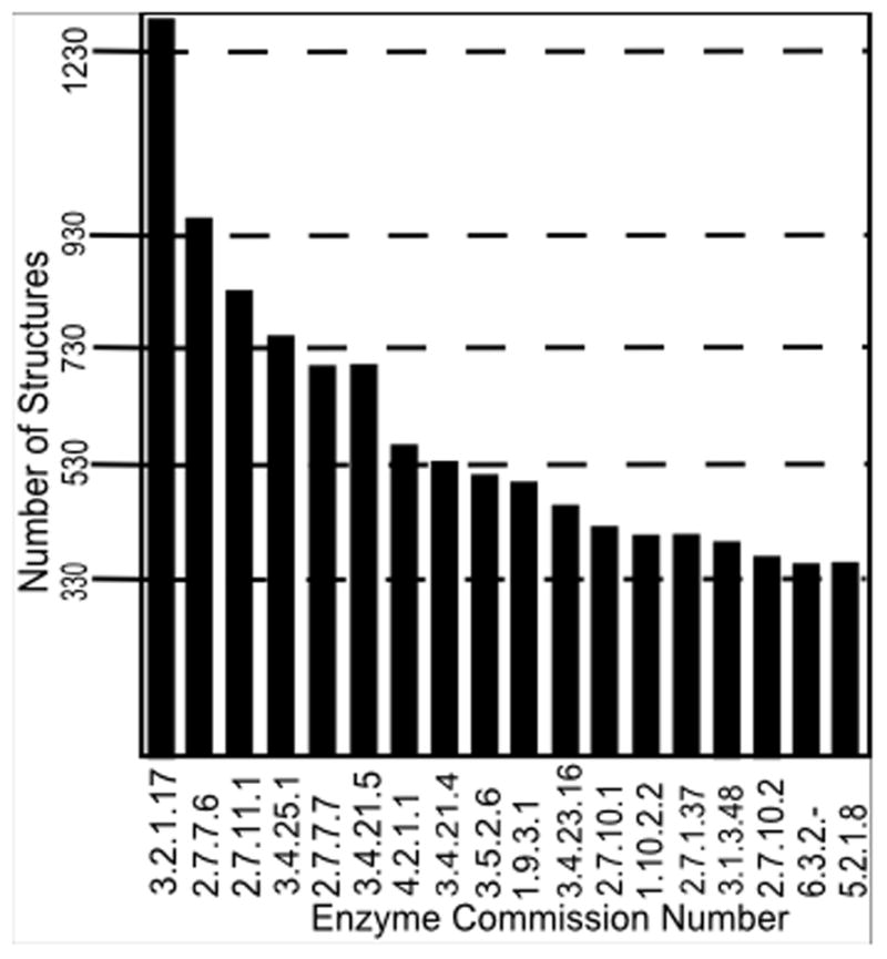
In total there are over 17,000 enzyme structures, and a significant number of structures for many diverse enzyme types. The most common structure on the left of this histogram with 1,285 structures is EC 3.2.1.17 that includes lysozymes, and at the right side is 5.2.1.8 acetylcholinesterases with 337 different structures (taken from enzyme classification histogram provided by PDB: http://www.pdb.org/pdb/statistics/histogram.do?mdcat=entity&mditem=pdbx_ec&name=Enzyme%20Classification) (1)).

Important conformational changes can readily be extracted from a set of PDB structures for a protein and these are found to relate directly to function. Experimental structures can be a rich source of information. It is well established that functionally related structures must have similar structures and similar dynamics – building on the broad experience of many researchers. There have been several efforts at extracting dynamics from specific sets of experimental structures. One approach is principal component analysis (PCA) (2–4), a statistical method based on covariance analysis. PCA can transform the original space of correlated variables into a greatly reduced space of independent variables (i.e., the principal components or PCs). By performing PCA, most of a system’s variance will usually be captured in a quite small subset of the PCs. PCA has been applied often to analyze trajectory data from MD simulations to find the essential dynamics (5;6). Teodoro et al. applied PCA to the dataset composed of many conformations for HIV-1 protease (7;8). They found that PCA transformed the original high-dimensional representation of protein motions into a low-dimensional one that provides the dominant protein motions. This is a huge reduction in dimensionality from hundreds of thousands to fewer than fifty degrees of freedom. Howe (9) used PCA to classify the structures in NMR ensembles automatically, according to correlated structural variations, and the results have shown that two different representations of the protein structure, the C^α coordinate matrix and the C^α-C^α distance matrix, gave equivalent results and permitted the identification of structural differences between conformations. More recent efforts include our own previous efforts in analyzing the HIV-1 protease set (10), those of the Bahar group (11), and our efforts in developing the MAVEN program (12), as well as related efforts by the Bahar group with their ProDy (13), and Grant with his Bio-3D (14). Any of these can provide a similar set of starting tools.

On the other hand, the Elastic Network Models (ENM) have proven themselves to be highly useful in representing the global motions for a wide variety of diverse protein structures (15–19). For modeling and simulating the dynamics of proteins, ENMs can be applied on multiple scales (20–23). All atom ENM models give a finer description of protein dynamics. The most common coarse-graining involves a single-site per residue representation, in which the sites are identified by the C^α atoms and connected by uniform springs. The dynamics of such interconnected model can be described by the Gaussian Network Model (GNM) (17) or the Anisotropic Network Model (ANM) (15). GNM has been very successful in yielding information on the magnitudes of the fluctuations of the protein structures but provides no directional information or the 3-D nature of motion of the protein is considered in the model. However, in reality protein fluctuations are generally directional and anisotropic (24;25). ANM considers the anisotropy of the protein structure in modeling its dynamics and thus ANM computed collective motions are more relevant to biological function and mechanism of the protein molecule.

In this chapter, we give an example of how to use computational methods to extract protein dynamics from a large set of experimental structures of HIV-1 protease. Behind this is the implicit assumption that there is a significant amount of information about protein dynamics, mechanisms and allostery buried within the structures in the PDB. We will show how to utilize PCA to extract dynamics from the abundantly available HIV-1 protease structures and how to compute the agreement between PCA-based protein motion and the ANM modeled motion, and describe how these could be used in simulations with a new structure-based elastic network model.

2 Theory

2.1 Principal Component Analysis (PCA)

PCA is a multivariate technique to analyze a dataset where the observations are described quantitatively by a set of inter-correlated variables. The goals of PCA are to (i) extract the most important information from the data; (ii) remove noise and compress the data set by keeping only the important information; (iii) simplify the description of the data set; and (iv) analyze the structure of the observations and the variables. This method generates a set of new orthogonal variables called principal components (PCs). Each PC is a linear combination of the original variables. Hence, PCA can be considered as a mapping of the data points from the original variable space to the PC space. PCs are rank ordered in such a way that PC1 represents the maximum variance among all possible choices for the first axis. Similarly, PC2 represents the second highest variance contribution, and so forth through all the modes. Usually only a few PCs are sufficient to understand the internal structure of the data (26).

For extracting functional dynamics from the PDB experimental structures, PCA is performed on the structure datasets. The input is the set of coordinates of all of the structures in the set (7;8). From these data, the average position of each point in the structure is computed as <r_i> and the covariances for pairs of points i and j are computed according to

$$c_{ij}=\langle (r_i-\langle r_i\rangle )(r_j-\langle r_j\rangle )\rangle$$ (1)

where brackets <> indicate averages over the entire set of structures. The covariance matrix C can be decomposed as

$$C=P\mathrm{\Delta }{P}^T,$$ (2)

where the eigenvectors P represent the principal components (PCs) and the eigenvalues are the elements of the diagonal matrix Δ. The eigenvalues are sorted in order. Each eigenvalue is directly proportional to the amount of the variance it captures.

2.2 Elastic Network Model (ENM)

Anisotropic Network Model (ANM) is an elastic network model used to compute the directions of the normal modes from a single structure (15). In ANM, the potential energy V is a function of the displacement vector D of each point in the structure

$$V=\frac{\gamma }{2}{\mathit{DHD}}^T,$$ (5)

where γ is the spring constant for all closely interacting points in a structure, and H is the Hessian matrix containing the second derivatives of the energy, with respect to each of the coordinates r = <x, y, z>. For a structure with n residues, the Hessian matrix H contains n × n super-elements of size 3 × 3. The Hessian matrix H can be decomposed (7;8;15) as

$$H=M\mathrm{\Lambda }{M}^T,$$ (6)

where Λ is a diagonal matrix comprising the eigenvalues with the eigenvectors forming the columns of the matrix M. This decomposition generates 3n-6 normal modes (the first 6 modes account for the rigid body translations and rotations of the system and must be factored out, meaning that we actually perform singular value decomposition to extract the normal modes) reflecting the vibrational fluctuations. We like to further mention that for ANM coarse graining, it is shown that a cutoff distance of any value from 10Å to 13 Å is appropriate for placing the springs and such an ANM model represents the realistic protein dynamics. In this chapter, we use a cutoff distance of 13 Å.

2.3 Structure-based new ANM

The internal distance changes in a set of structures can provide information that can be used directly to derive new structure-based elastic network models. We have extracted spring constants between all residue pairs in a set of structures by simply relating these to the inverse of the variance of internal distance changes between pairs of residues, as the spring stiffness (normalized between 0 and 1). We have applied a cutoff of 13Å to limit the range of interactions. However the difference between the conventional ANM described in the previous section and this modified ANM is that here the values for the spring constants are obtained directly from the structure set rather than using a uniform value or distance dependent values, as is customary with ENM.

2.4 Comparing directions of motions using Overlaps

The alignment between the directions of motion, for example between a given PC and a given normal mode, is measured by their overlap, which was defined as the dot product of the two vector directions by Tama and Sanejouand (27)

$$O_{ij}=\frac{\left|P_i·M_j\right|}{\Vert P_i\Vert \Vert M_j\Vert },$$ (3)

where P_i is the i^th PC for model P and M_j is the j^th PC or normal mode for model M. A perfect match yields an overlap value of 1. They also defined the cumulative overlap (CO) between the first k vectors of M and P_i as

$$\text{CO}(\mathrm{k})={\left(\sum _{\mathrm{j}=1}^{\mathrm{k}}{\mathrm{O}}_{ij}^2\right)}^{\frac{1}{2}}$$ (4)

which measures how well the first k PCs for model M together can capture the motion of a single PC for model P.

2.5 Coarse-grained global Entropies calculated from Principal Component Analysis

As covariance matrix can be decomposed as in equation 2 of section 2.1, an approximation of the entropy from the PCs can be obtained as well (10;28):

$$\mathrm{\Delta }\mathrm{S}=\text{Const}\sum _{\mathrm{i}=1}^{\mathrm{N}}{\mathrm{\lambda }}_{\mathrm{i}}\left({\text{PC}}_{\mathrm{i}}{\text{PC}}_{\mathrm{i}}^{\mathrm{T}}\right)$$ (1)

where PC_i is the i^th PC, and λ_i is the i^th eigenvalue, N is the total number of eigenvalues.

Andricioaei, I et al also reported a similar result for entropy calculation from the covariance matrices of the atomic fluctuations as shown in equation 7 of their paper (29). It should be noted that this expression is different from that for normal modes of the elastic network models, which because of the averaging normally involved the inverse of the eigenvalues.

3 Materials

There are a huge number of available HIV-1 protease structures in the PDB (564 X-ray and three NMR structures as of 07/26/2013), which provides a remarkably rich set of different conformational states, which can be viewed as direct structural information on the protein’s dynamics.

The approach described here computes the essential or most important protein motions from multiple structures of the same protein, in contrast to using just the two structures such as the “open” and “closed” conformations, which have often been used to define the endpoints of conformational transitions. To demonstrate this approach, we use HIV-1 protease as an example. Its abundant experimentally determined structures are complemented by the relatively small size of the protein. In the next section, first, we will give a description of the structural components that are important to drive the motion of the HIV-1 protease structure. Then, we will describe the dataset of HIV-1 structures that we have used to perform our computations.

3.1 HIV-1 Protease Architecture

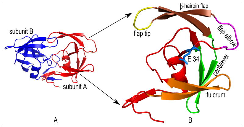
HIV-1 protease functions as a homo-dimer as shown in Fig. 2A. The dimer has a single active site and 99 residues per monomer. Each monomer has three domains: a terminal domain (residues 1–4 and 95–99 of each chain), which is important for the dimerization and stabilization; a core domain (residues 10–32 and 63–85 of each chain), for dimer stabilization and catalytic site stability; and a flap domain that includes two solvent accessible loops (residues 33–43 of each chain) followed by two flexible flaps (residues 44–62 of each chain) important for ligand binding interactions. The conserved Asp25-Thr26-Gly27 active site triad is located at the interface between parts of the core domains. The active site of HIV-1 protease is formed at the homo-dimer interface. Each monomeric unit has important structural components as identified in Fig. 2B that are important for its functional dynamics. The principal advantage of this structural arrangement is that the hinge residue E 34 causes the up-down swinging motion of the flap elbow (residues 37 – 42), which transmits the motion generated in the fulcrum (residues 9 – 21) to drive the dynamics of the flap domain (residues 42 – 58), whose conformation switches between open and closed states to facilitate substrate trapping in the catalytic pocket and product release following hydrolysis (30;31).

Figure 2. Description of HIV-1 protease homo-dimer and its critical structural components that facilitate the functional dynamics.

(A) HIV-1 protease has two symmetric subunits – subunit A (red) and subunit B (blue). (B) Each subunit has several structural components that are important for its coordinated motions. Fulcrum (orange, residues 9 – 21) is a comparatively less mobile region that swings up and down similar to the flap elbow. E-34 (blue) – Hinge residue which is responsible for transmitting the motion from the fulcrum to the flap region. Flap elbow (magenta, residues 37 – 42) – Hinge residue E-34 drives the motion of this region to transfer the dynamics further away from the fulcrum to the upper flap region. This loop can make top-down and bottom-up swings. When the flap elbow swings from top to bottom, the flap domain opens up, and when it swings upward the flap domain closes. The Flap domain (residues 43 – 58) consists of flap tip (yellow, residues 49 – 52) and β-hairpin flaps (dark orange, residues 43 – 48 and 53 – 58). Opening and closing of the flap domains enable the protein to bind ligands and release its products after proteolysis. Cantilever (green, residues 59 – 75) functions as a base for the flap domain. The C-terminal β-hairpin flap is held by the N-terminal end of the cantilever and this arrangement is important to control the swinging of the flap (30;31).

3.2 HIV-1 protease structure set (X-ray-329)

We have used 329 PDB structures of HIV-1 protease for the computations to extract protein dynamics from experimental structures. The PDB Ids of the data set are here:

1A30

1A8G

1A8K

1A94

1A9M

1AAQ

1AID

1AJV

1AJX

1AXA

1B6J

1B6K

1B6L

1B6M

1B6P

1BDL

1BDQ

1BDR

1BV7

1BV9

1BWA

1BWB

1C6X

1C6Y

1C6Z

1C70

1D4S

1D4Y

1DAZ

1DIF

1DMP

1DW6

1EBK

1EBW

1EBY

1EBZ

1EC0

1EC1

1EC2

1EC3

1F7A

1FEJ

1FF0

1FFF

1FFI

1FG6

1FG8

1FGC

1FQX

1G2K

1G35

1GNM

1GNN

1GNO

1HBV

1HIH

1HIV

1HOS

1HPO

1HPS

1HPV

1HPX

1HSG

1HSH

1HTE

1HTF

1HTG

1HVH

1HVI

1HVJ

1HVK

1HVL

1HVR

1HVS

1HWR

1HXW

1IIQ

1IZH

1IZI

1K1U

1K2B

1K2C

1K6C

1K6P

1K6T

1K6V

1KJ4

1KJ7

1KJF

1KJG

1KJH

1LZQ

1M0B

1MER

1MES

1MET

1MEU

1MRW

1MRX

1MSM

1MSN

1MT7

1MT8

1MT9

1MTB

1MTR

1MUI

1N49

1NH0

1NPA

1NPV

1NPW

1ODW

1ODX

1PRO

1QBR

1QBS

1QBT

1QBU

1RL8

1RPI

1RQ9

1RV7

1SDT

1SDU

1SDV

1SGU

1SH9

1SP5

1T3R

1T7I

1T7J

1T7K

1TCX

1TW7

1U8G

1VIJ

1VIK

1XL2

1XL5

1YT9

1YTG

1YTH

1Z8C

1ZBG

1ZLF

1ZPK

1ZSF

1ZSR

2A1E

2A4F

2AID

2AOF

2AQU

2AVM

2AVO

2AVS

2AVV

2AZC

2B7Z

2BB9

2BBB

2BPV

2BPW

2BPX

2BPY

2BPZ

2BQV

2CEJ

2CEM

2CEN

2F3K

2F80

2F81

2F8G

2FDD

2FDE

2FGU

2FGV

2FNS

2FNT

2FXD

2FXE

2HB3

2HC0

2HS1

2HS2

2I4D

2I4U

2I4V

2I4W

2I4X

2IDW

2IEN

2IEO

2J9J

2J9K

2JE4

2NMZ

2NNK

2NNP

2O4K

2O4L

2O4P

2O4S

2P3A

2P3B

2P3C

2P3D

2PK5

2PK6

2PQZ

2PWC

2PWR

2PYM

2PYN

2Q3K

2Q63

2Q64

2QAK

2QCI

2QD6

2QD7

2QD8

2QHC

2QHY

2QHZ

2QI0

2QI1

2QI3

2QI4

2QI5

2QI6

2QI7

2QMP

2QNN

2QNP

2QNQ

2R38

2R3T

2R3W

2R43

2R5P

2R5Q

2RKF

2UPJ

2UXZ

2UY0

2Z4O

3A2O

3AID

3BGB

3BGC

3BVA

3BVB

3CKT

3CYW

3CYX

3D1X

3D3T

3FX5

3GGA

3GGV

3GGX

3GI4

3GI5

3GI6

3I7E

3KF0

3KFN

3KFR

3KFS

3LZS

3LZU

3MWS

3NDU

3NDX

3NU3

3NU4

3NU5

3NU6

3NU9

3NUJ

3NUO

3O9F

3O9G

3O9H

3O9I

3OK9

3OTS

3OXC

3PWM

3PWR

3QAA

3R4B

3S43

3S53

3S54

3S56

3S85

3SO9

3T11

3U7S

3UCB

3UF3

3UHL

4DQB

4DQC

4DQE

4DQG

4DQH

4EJ8

4EJK

4EJL

4FAE

4FL8

4FLG

4FM6

4HVP

4I8W

4I8Z

4J54

4J55

4J5J

4PHV

7HVP

7UPJ

8HVP

9HVP

The following method section gives a step by step description of how to retrieve these PDB files from the protein databank and then how to extract the dynamics from these structures.

4 Methods

To successfully complete the procedures described in this section, one needs the following softwares/programs:

• Perl 5 – Several perl scripts are included here. Perl programming language (32) can be downloaded free at www.perl.org.

• Python – A python script is used to calculate the internal distances between residue pairs for the set of 329 protein structures. A Python environment can be downloaded at http://www.python.org/

• Matlab – Several Matlab scripts are included here that can be executed in a Matlab programming environment (33). Matlab product site is http://www.mathworks.com/products/matlab/

• MAVENs – This software was developed in the Jernigan lab (12). In our Matlab code, we have invoked several MAVEN functions –

  • ANM.m – This is a function from MAVEN (12) used in experimentalDynamics.m to compute ENM normal modes from a given PDB structure.

  • modeAnimator.m – This is a function from MAVEN used in experimentalDynamics.m to visualize the ENM modes and PCs by creating movies.

  • readPDB.m, writePDB.m – These two Matlab functions from MAVEN are used to read and write PDB files, respectively.

  • CompareVectors.m – This function from MAVEN is used in experimentalDynamics.m to compare the directions of PCs and ENM modes.

  • plot_compareVectors.m – This function from MAVEN plots the results obtained from the above CompareVectors.m.

  • mat2vec.m – This function converts a matrix to a vector.

    MAVEN is available for download at http://maven.sourceforge.net.

• MUSTANG – Multiple structural alignment will be done using this program (34). This program can be installed only on a linux operating system. You can download MUSTANG can be downloaded at http://www.csse.monash.edu.au/~karun/Site/mustang.html.

• PyMOL – This software has a free version for academic use (35). This can be used to visualize the structures and their dynamics. PyMOL can be downloaded at http://pymol.org/.

The following Table I summarizes the steps that are discussed in this section – starting from processing raw PDB structures to computing PCs and ANM modes, and comparing their dynamics.

Table I.

Summary of the steps for extracting biomolecular dynamics

§4.1 Extracting Cartesian coordinates from raw PDB files §4.1.1 Data set preparation for MUSTANG from raw PDB files
Program/File Name	Function
copyBackboneAtoms.pl	Copies backbone ATOM and HETATM from a set of PDB files.
retainFirstAltLocation.pl	Retains the first alternate location for each ATOM and HETATM when multiple locations for that ATOM/HETATM exist. It operates on a set of PDB files.
replaceHETATM.pl	Replaces the keyword HETATM with the keyword ATOM in a set of PDB files.
retainCA.pl	Copies the CA atoms from a set of PDB files with no TER keyword between chains to comply with the MUSTANG input file format.
§4.1.2 Multiple structural alignment using MUSTANG §4.1.3 Data set preparation for PCA from MUSTANG output
copyChainsToPDBs.pl	Copies the chains from alignAll.pdb to individual PDB files.
pdbIds.txt	This file list the PDB ids for 329 PDB structures used here.
§4.2 Principal Component Analysis (PCA) §4.3 Comparing and visualizing PCs and ANM modes §4.4 Comparing PCs and structure-based ANM §4.5 Computing Entropy using PCs
experimentalDynamics.m	This Matlab program (i) computes principal components from aligned structures, (ii) computes ENM modes, (iii) computes the overlap between PCs and ENM modes, (iv) computes entropies from PCs.
readAlignedPDBcoordinates.m	This Matlab function reads the coordinates of aligned PDB structures and returns the coordinates of those structures.
internal.py	This program, written in Python, calculates the internal distances of Mustang aligned structures.
calc_Entropy_PC.m	This Matlab function computes entropy from computed PCs.

The above files, the files used from MAVEN, other accessory files and dataset can be downloaded at http://ribosome.bb.iastate.edu/4papers/2013/ataur/experimentalDynamics/

4.1 Extracting Cartesian coordinates from raw PDB files

In this section, we will describe how to prepare the dataset X-ray-329 for PCA. The 329 PDB Ids are listed in the pdbIds.txt file. Download these files from the protein data bank (http://www.pdb.org/pdb/download/download.do) (Download options: download Type – PDB File Format, Compression Type – uncompressed) and save them in a sub folder named data-raw under the parent folder experimentalDynamics. The downloaded PDB files have a lot of extra information that we will not be used.

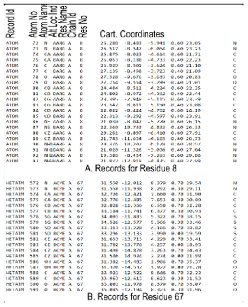
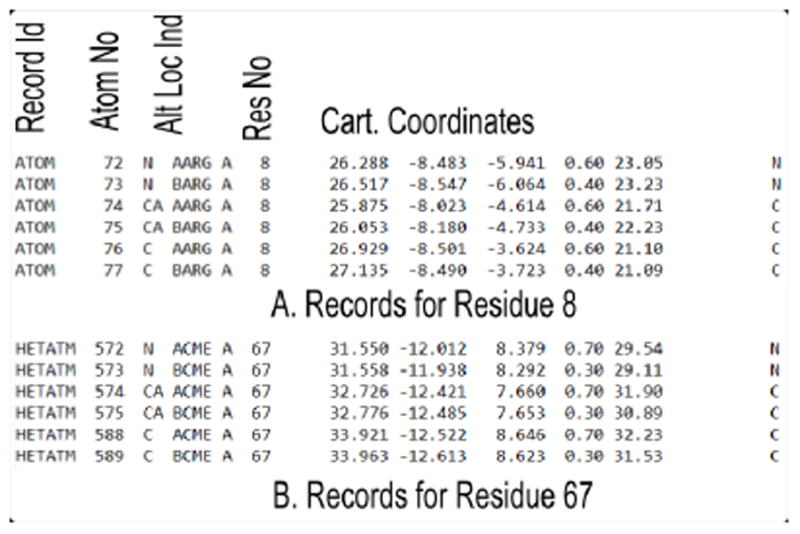
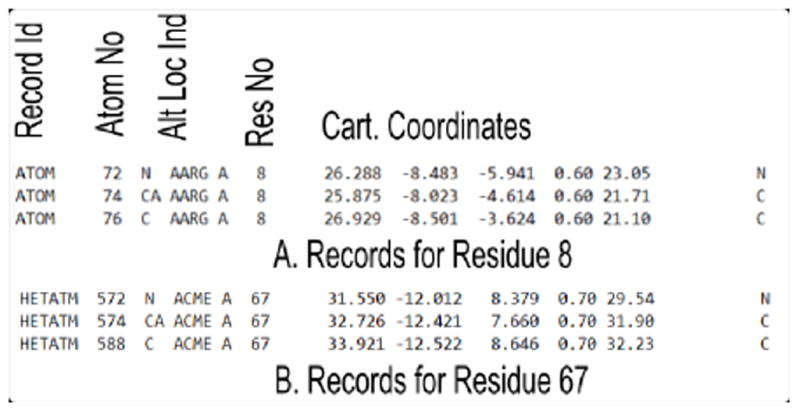
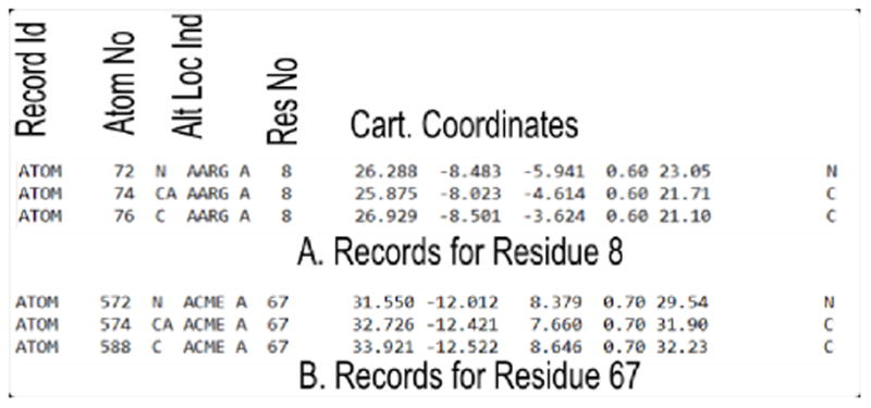
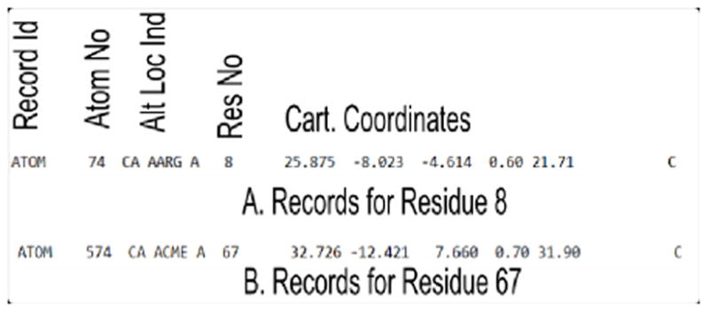
The records of ATOM type for residue 8 and modified residue 67 of PDB file 2p3a are shown below. The important fields are labeled. Each residue of a protein is recorded in this way. When a residue in the protein is modified with a non-amino acid type molecule, HETATM keyword is used to identify that record. The TER key word is used as an end of chain marker. The PDB file has other detailed information and have different record identifiers. We will retain the ATOM type records for the C^α atoms of each residue or modified residue for our calculation. When more than one alternate location is recorded, we arbitrarily retain the first alternate location for that ATOM.

The following three subsections describe how to copy the Cartesian coordinates from each PDB file and align these structures.

4.1.1 Preparing a data set for MUSTANG from raw PDB files

Download and save the following perl scripts in the same folder – experimentalDynamics. Run these perl scripts in the same sequence as they are listed below:

• copyBackboneAtoms.pl – This program copies the backbone ATOM and HETATM from a set of PDB files.

  • perl copyBackboneAtoms.pl

  • Output files after running this program will be saved in data-backbone subfolder of the experimental Dynamics parent folder.

  • Running this program will retain the backbone atoms for each ATOM and HETATM record. A sample output for residue 8 and modified residue 67 is shown below.

• retainFirstAltLocation.pl – This program retains the first alternate location for each ATOM when multiple alternatate locations for that ATOM exist. It operates on a set of PDB files.

  • perl retainFirstAtlLocation.pl

  • Output files after running this program will be saved in data-backbone-singleAltLocation subfolder of the experimentalDynamics parent folder.

  • After running this program, a PDB file will have residues with only the backbone atoms and only the first alternate location will be retained in case of multiple alternate locations. Output for residue 8 and modified residue 67 is shown below.

• replaceHETATM.pl – This program replaces the keyword HETATM with the keyword ATOM in a set of PDB files.

  • perl replaceHETATM.pl

  • Output files after running this program will be saved in data-backbone-singleAltLocation-NoHETATM subfolder of the experimentalDynamics parent folder.

  • MUSTANG (34) removes all records with the keyword HETATM before multiple structural alignment. To prevent the removal of needed data, replaceHETATM.pl program replaces the keyword HETATM with ATOM so that MUSTANG will use the HETATM coordinates as required in the multiple structure alignment. Sample output for residue 8 and modified residue 67 is shown below:

• retainCA.pl – This program copies the CA atoms from a set of PDB files.

  • perl retainCA.pl

  • Output files after running this program will be saved in data-CA subfolder of the experimentalDynamics parent folder.

  • This program retains the records of the C^α atoms only. Therefore, for each residue only the record for C^α will be copied. Also, the TER keyword to separate the chains will not be retained in the output file so that MUSTANG considers the whole structure (multiple chains) as one chain. A sample output for residue 8 and modified residue 67 is shown below:

4.1.2 Aligning PDB structures using MUSTANG

There are several successful multiple structural alignment programs such as MUSTANG (34), TM-align (36), DaliLite (37), etc. A Wikipedia page has a list of multiple structure alignment softwares/programs (http://en.wikipedia.org/wiki/Structural_alignment_software, 10/15/2013). We have used MUSTANG for multiple structural alignments of the selected PDB structures. MUSTANG does not consider sequence information in its alignment algorithm. Rather, it performs a structural alignment by finding maximal similar substructures. Thus it can capture the conformational variations among the structures much better than the alignment algorithms that rely upon sequence similarity information. Moreover, in its alignment MUSTANG uses the C^α backbone atoms only. The running time MUSTANG 3.2.1 for the alignment of the selected dataset of 329 structures is approximately 5.00 hours on a Linux machine with the following configuration – Linux version 2.6.18-348.4.1. el5 Intel(R) Xeon(R) CPU E5630 @2.53GHz. MUSTANG needs a linux operating system. After installing MUSTANG under the experimentalDynamics folder on a linux machine, save and copy the following file description in the same folder; and copy data-CA subfolder with the structures in the same folder as well:

• data-CA: This folder has all the backbone PDB files for multiple structural alignments.

• description: This file has the path of the source directory where MUSTANG will find the input files for multiple structural alignment. After the path information, this file also has the list of the PDB file names that MUSTANG will read from the source directory. The list of the filenames in this file is in the same order as the list of the PDB Ids in the pdbIds.txt file which has the 329 PDB Ids that are listed in section 3.2. Update the line in description file that records the path of the source directory for the input files (path to the files in data-CA subfolder) that would be aligned.

Run the following command to execute MUSTANG:

• mustang-3.2.1 -f description -o alignAll -F fasta -r ON

This will create the following two files:

• alignAll.pdb: This file contains the aligned structures. Each chain corresponds to a specific PDB file and the header of this file lists the file names in the same order.

• alignAll.afasta: This contains the alignment of the amino acid sequences of the HIV-1 proteases based on the structural alignment.

4.1.3 Preparing data for PCA from MUSTANG output files

• copyChainsToPDBs.pl – This perl script will copy each chain of alignAll.pdb file to the corresponding PDB file according to PDB Ids listed in the pdbIds.txt file.

  • perl copyChainsToPDBs.pl pdbIds.txt alignAll.pdb

This will create a subfolder aligned PDBs in the experimentalDynamics folder. This subfolder will have the 329 PDB files with the aligned C^α atoms of each structure. So when the Cartesian coordinates of each file will be placed in a matrix such that each row corresponds to the coordinates of one PDB Id, this matrix can be used for principal component analysis.

4.2 Use of Cartesian PCs to extract functional dynamics from the protein structures

Matlab script experimentalDynamics.m reads the Cartesian coordinates of the structures from the MUSTANG aligned files and perform PCA on them.

4.2.1 Significance of Principal Components (PCs)

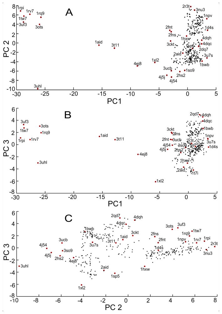
Figure 3 shows the distribution of the 329 PDBs Ids projected onto the space of the first few PCs from three separate views – PC1-PC2 (panel A), PC1-PC3 (panel B), and PC2-PC3 (panel C). In panels A and B, open and closed structures are clearly separated in two regions (open structures on the left side and closed structures on the right side) and the intermediate conformations (1aid, 3t11, 4ej8, etc) spanning the middle region. The PC2-PC3 view in panel C, the structures are distributed based on conformational differences in the flap elbow region.

Figure 3. Distributions of the 329 PDB structures by PCA.

(A) Distribution of the structures on a PC1-PC2 plot. (B) Distribution of the structures on a PC1-PC3 plot. (C) Distribution of the structures on a PC2-PC3 plot. In plots A and B, open structures are located on the left side; closed structures are located on the right side; and the intermediate structures fall in between. Distribution of structures on PC2-PC3 plot (panel C) is based on primarily on the conformational differences along the flap elbow region. PC1, PC2, and PC3 capture 30%, 20%, and 7% of the variances in the dataset, respectively.

We used the MAVEN function modeAnimator.m to animate the motions of the structure along PC1, PC2, and PC3 vectors. The following code calculates the conformations along PC1 and can be found in experimentalDynamics.m matlab function:

m = readPDB(ifname,1); %read the MUSTANG reference structures
c = sqrt(length(m.IND)/ sum(PC(:,1).^2));
%c controls the vector displacement amount
modeAnimator(m,PC(:,1),’’,c,c/10 ,ofname,’’,0,’’,1);
%use PC1 as the mode vector to simulate the motion of the structure

The motion of the structure along PC1, PC2, and PC3 can be observed by opening the corresponding file using PyMOL visualization software. It is evident that, PC1 is closely related to the opening and closing (or expansion/contraction) of the flaps and the ligand binding cavity as shown in Fig. 4A. The two extreme ends of PC1 motion correspond closely to the closed (+) and the open (−) experimental structures (closed: PDB 1ebw, open: PDB 1rpi). The PC2 and PC3 correspond to twisting motions that are best seen in a perpendicular direction to those of PC1. PC2 is predominantly a twisting motion of the flap domains (panel C), whereas PC3 is predominantly a hinge motion of the core domains moving towards and away from the flaps (panel D).

Figure 4. Visualization of the first three PCs of HIV-1 protease on the structures.

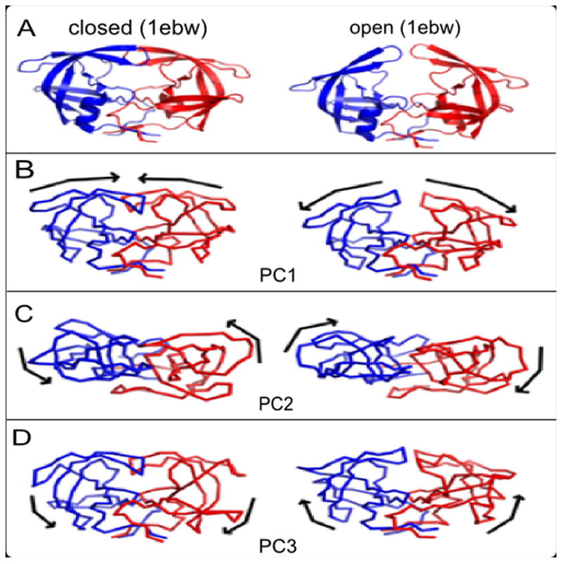
(A) Structures showing the closed form (left, PDB 1ebw) and open form (right, PDB 1rpi) of HIV-1 protease. The two subunits are shown in red and blue color and in ribbon diagram. (B) Snapshots of the structures displaced along the directions of PC1 shown in connected line segement. The direction of motions of the protein along each PC is shown with a black arrow. It can be seen that the opening-closing motion of the flaps can be easily identified from the extrema of PC1. Two extrema are shown for each motion in each row, together with arrows that indicate the directions for transition to the other structure. (C) PC2 images are shown looking down from the top of those in PC1 and PC3. PC2 is a twisting of the flap regions whereas (D) PC3 is a hinge motion between the core and flaps, with the core and flaps moving to and fro relative to one another.

experimentalDynamics.m also has code to visualize structures by using the ANM modes and the generated frames are saved in PDB file format that can be visualized using PyMOL software.

4.2.2 Comparing PC based and ANM computed dynamics

Matlab program experimentalDynamics.m has the code to compute the ANM modes by using the MAVEN function ANM.m, and it then computes the overlap and the cumulative overlaps with the previously computed PCs by using another MAVEN function CompareDynamics.m. Figure 5, generated by MAVEN function plot_compareDynamics.m, shows the overlaps between the first 10 PCs and the first 10 ANM modes. The highest overlap is 60% found between PC1 and ANM mode 3.

Figure 5.

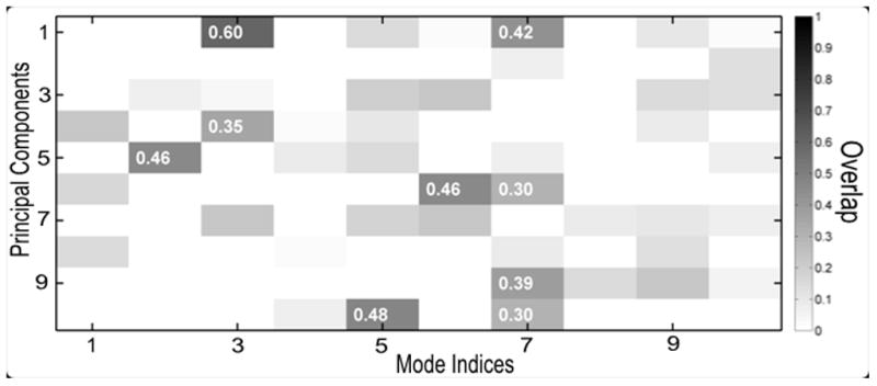
Overlap between PCs and ANM modes. PC1 and mode 3 gives the highest overlap 60%.

Table II shows the cumulative overlaps between PCs and the ANM modes. The cumulative overlap between each of the first and the second PCs and the first 20 modes is above 80%. Interestingly, the cumulative overlap reaches 80% between the second PC and the first 6 modes. This clearly indicates that given an appropriate experimental dataset the motions captured by the PCs conform quite closely with the ANM motions.

Table II.

Cumulative Overlap between the first three PCs and sets of the ANM modes

ANM Modes/PCs	PC1	PC2	PC3
3 modes	0.62	0.71	0.44
6 modes	0.64	0.80	0.54
10 modes	0.77	0.83	0.59
20 modes	0.80	0.85	0.65

^*CO between a PC and ANM modes is shown in bold type if it is greater than 0.80

4.3 New internal distance based ANM motions

The use of structural information in ANM improves the modeling of the protein dynamics. Section 2.3 describes a way to derive spring constants from the structures. Here, we compute the inverse of the variance of the internal distances from the aligned structures in the MUSTANG aligned file align. pdb by using the Python program internal. py. The calculated inverse values are stored in hiv.329.var.sc file that could be downloaded at the link in the footnote of Table I. MAVEN function ANM.m can be modified to use these values as the spring constants to compute the normal modes. Table III shows the overlaps of PCs based on these internal distances and the new ANM modes. The highest overlap is 79% that occurs between PC1 and mode 2, which is much higher than the highest overlap (60%) that occurred between PCs and conventional ANM modes (Fig. 5).

Table III.

Overlaps between PCs and the new ANM modes

PCs/newANM Modes	Mode 1	Mode 2	Mode 3
PC1	0.09	0.79	0.40
PC2	0.34	0.01	0.24
PC3	0.34	0.01	0.10

Table IV shows the cumulative overlap between PCs and the new ANM modes. We can see that cumulative overlap between PC1 and the first three modes reaches 90% which is quite high compared to the cumulative overlap between PC1 and the first three modes (62% as shown in Table II). However, the cumulative overlap between PC2 and the first three modified ANM 42%; on the other hand this value between PC2 and the first three conventional ANM modes is 71%, a much higher value. Therefore, in some cases cumulative overlap between a PC and the new ANM modes gets improved compared to the similar values between a PC and the conventional ANM modes. But when 20 new ANM modes are included, the values are constantly higher.

Table IV.

Cumulative overlaps between PCs and the new ANM modes

New ANM modes/PCs	PC1	PC2	PC3
3 Modes	0.90	0.42	0.35
6 Modes	0.91	0.44	0.41
20 Modes	0.95	0.89	0.84

Values in bold indicate cumulative overlaps above 80%

Taken together, this suggests that modified ANM can improve the performance of the ANM models.

4.4 Computing Entropy using PCs

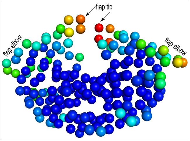
We compute the entropy of the HIV-1 protease system using equation 2 described in section 2.5. By using calc_Entropy_PC.m matlab program, we compute the entropy from the principal components of the 329 aligned HIV-1 protease structures. The residues of HIV-1 protease are colored in Fig. 6 according to the entropy values. It is clear from the figure that the entropies are asymmetrically distributed in the two HIV-1 protease subunits. Subunit A (right subunit) has higher entropies along the flap and flab elbow regions.

Figure 6. Depiction of entropies of HIV-1 protease structure (PDB 1rpi) computed from PCs.

Residues are colored spectrally according to the entropy values – coloring from red for the highest entropy to blue for the lowest entropy. Some of the residues along the flap and flap elbow regions on the subunit A (right subunit) have higher entropies than the same residues on subunit B (left subunit).

5 Conclusion

This chapter gives the background of two important methods – PCA and ENM. By following the steps with the set of 329 HIV-1 PDB structures, one can get a hands-on experience on how to apply PCA to extract dynamics and mechanism information by capturing the conformational variability buried in different PDB structures of the same protein. One can also learn how to model the functionally important global motions of the protein using the widely accepted ANM model and compare the dynamics and mechanism found from experimental structures by PCA and from the ANM model. The higher overlaps between PCs and modified ENM modes indicate that a rich dataset of protein structures can play an important role in understanding functional dynamics and mechanism of the protein.

Moreover, the PC’s represent the variability apparent within the sets of structures, and hence these are used as a direct measure of the conformational entropy of the protein structure.

This approach can also be extended to other highly diverse protein structure sets. The PDB database continues to grow rapidly – in 2008 there were ~43,000 protein structures and now in 2013 there are more than 90,000 structures (1). In the future if new technologies for X-ray structure determination are developed that are much more efficient and very rapid, then there will be truly abundant structures of related proteins, including aberrant protein structures from patients. Among the various structures there are many single proteins with multiple X-ray structures determined under different conditions, as well as NMR structures. Generally proteins are robust and not easily disturbed by different environments or mutations; and the preponderance of evidence suggests that proteins have a limited range of conformations that are essential for their function. Therefore, the approach described here can generally be used to extract dynamics of any protein with significant numbers of available experimental structures.

Schema 1.

Schema 2.

Schema 3.

Schema 4.

Schema 5.

References

- 1.Berman HM, Westbrook J, Feng Z, Gilliland G, Bhat TN, Weissig H, Shindyalov IN, Bourne PE. The Protein Data Bank. Nucleic Acids Res. 2000;28(1):235–242. doi: 10.1093/nar/28.1.235. [DOI] [PMC free article] [PubMed] [Google Scholar]
- 2.Hotelling H. Analysis of a complex of statistical variables into principal components. Journal of Educational Psychology. 1993;24:417–441. [Google Scholar]
- 3.Manly B. Multivariate statistics - A primer. Chapman & Hall/CRC; Boca Raton: 1986. [Google Scholar]
- 4.Pearson K. On lines and planes of closest fit to systems of points in space. Philosophical Magazine and Journal of Science. 1901;2(6):559–572. [Google Scholar]
- 5.Amadei A, Linssen AB, Berendsen HJ. Essential dynamics of proteins. Proteins. 1993;17:412–425. doi: 10.1002/prot.340170408. [DOI] [PubMed] [Google Scholar]
- 6.Amadei A, Linssen AB, de Groot BL, van Aalten DM, Berendsen HJ. An efficient method for sampling the essential subspace of proteins. J Biomol Struct Dyn. 1996;13:615–625. doi: 10.1080/07391102.1996.10508874. [DOI] [PubMed] [Google Scholar]
- 7.Teodoro ML, Philips GN, Jr, Kavraki LE. A dimensionality reduction approach to modeling protein flexibility. Int Conf Comput Mole Biol(RECOMB) 2002:299–308. [Google Scholar]
- 8.Teodoro ML, Philips GN, Jr, Kavraki LE. Understanding protein flexibility through dimensionality reduction. J Comput Biol. 2003;10:617–634. doi: 10.1089/10665270360688228. [DOI] [PubMed] [Google Scholar]
- 9.Howe PW. Principal components analysis of protein structure ensembles calculated using NMR data. J Biomol NMR. 2001;20:61–70. doi: 10.1023/a:1011210009067. [DOI] [PubMed] [Google Scholar]
- 10.Yang L, Song G, Carriquiry A, Jernigan RL. Close correspondence between the motions from principal component analysis of multiple HIV-1 protease structures and elastic network modes. Structure. 2008;16:321–330. doi: 10.1016/j.str.2007.12.011. [DOI] [PMC free article] [PubMed] [Google Scholar]
- 11.Yang LW, Eyal E, Bahar I, Kitao A. Principal component analysis of native ensembles of biomolecular structures (PCA_NEST): insights into functional dynamics. Bioinformatics. 2009;25:606–614. doi: 10.1093/bioinformatics/btp023. [DOI] [PMC free article] [PubMed] [Google Scholar]
- 12.Zimmermann MT, Kloczkowski A, Jernigan RL. MAVENs: motion analysis and visualization of elastic networks and structural ensembles. BMC Bioinformatics. 2011;12:264. doi: 10.1186/1471-2105-12-264. [DOI] [PMC free article] [PubMed] [Google Scholar]
- 13.Bakan A, Meireles LM, Bahar I. ProDy: protein dynamics inferred from theory and experiments. Bioinformatics. 2011;27:1575–1577. doi: 10.1093/bioinformatics/btr168. [DOI] [PMC free article] [PubMed] [Google Scholar]
- 14.Grant BJ, Rodrigues AP, ElSawy KM, McCammon JA, Caves LS. Bio3d: an R package for the comparative analysis of protein structures. Bioinformatics. 2006;22:2695–2696. doi: 10.1093/bioinformatics/btl461. [DOI] [PubMed] [Google Scholar]
- 15.Atilgan AR, Durell SR, Jernigan RL, Demirel MC, Keskin O, Bahar I. Anisotropy of fluctuation dynamics of proteins with an elastic network model. Biophys J. 2001;80:505–515. doi: 10.1016/S0006-3495(01)76033-X. [DOI] [PMC free article] [PubMed] [Google Scholar]
- 16.Bahar I, Jernigan RL. Cooperative structural transitions induced by non-homogeneous intramolecular interactions in compact globular proteins. Biophys J. 1994;66:467–481. doi: 10.1016/s0006-3495(94)80798-2. [DOI] [PMC free article] [PubMed] [Google Scholar]
- 17.Bahar I, Atilgan AR, Erman B. Direct evaluation of thermal fluctuations in proteins using a single-parameter harmonic potential. Fold Des. 1997;2:173–181. doi: 10.1016/S1359-0278(97)00024-2. [DOI] [PubMed] [Google Scholar]
- 18.Bahar I, Erman B, Haliloglu T, Jernigan RL. Efficient characterization of collective motions and interresidue correlations in proteins by low-resolution simulations. Biochemistry. 1997;36:13512–13523. doi: 10.1021/bi971611f. [DOI] [PubMed] [Google Scholar]
- 19.Bahar I, Jernigan RL. Inter-residue potentials in globular proteins and the dominance of highly specific hydrophilic interactions at close separation. J Mol Biol. 1997;266:195–214. doi: 10.1006/jmbi.1996.0758. [DOI] [PubMed] [Google Scholar]
- 20.Bahar I, Rader AJ. Coarse-grained normal mode analysis in structural biology. Curr Opin Struct Biol. 2005;15:586–592. doi: 10.1016/j.sbi.2005.08.007. [DOI] [PMC free article] [PubMed] [Google Scholar]
- 21.Chennubhotla C, Rader AJ, Yang LW, Bahar I. Elastic network models for understanding biomolecular machinery: from enzymes to supramolecular assemblies. Phys Biol. 2005;2:S173–S180. doi: 10.1088/1478-3975/2/4/S12. [DOI] [PubMed] [Google Scholar]
- 22.Jernigan RL, Yang L, Song G, Doruker P. Elastic Network Models of Coarse-Grained Proteins Are Effective for Studying the Structural Control Exerted over Their Dynamics. In: Voth G, editor. Coarse-Graining of Condensed Phase and Biomolecular Systems. Taylor and Francis Group LLC. CRC Press; 2008. pp. 237–254. [Google Scholar]
- 23.Bahar I. On the functional significance of soft modes predicted by coarse-grained models for membrane proteins. J Gen Physiol. 2010;135:563–573. doi: 10.1085/jgp.200910368. [DOI] [PMC free article] [PubMed] [Google Scholar]
- 24.Ichiye T, Karplus M. Anisotropy and anharmonicity of atomic fluctuations in proteins: analysis of a molecular dynamics simulation. Proteins. 1987;2:236–259. doi: 10.1002/prot.340020308. [DOI] [PubMed] [Google Scholar]
- 25.Kuriyan J, Petsko GA, Levy RM, Karplus M. Effect of anisotropy and anharmonicity on protein crystallographic refinement. An evaluation by molecular dynamics. J Mol Biol. 1986;20:190, 227–254. doi: 10.1016/0022-2836(86)90295-0. [DOI] [PubMed] [Google Scholar]
- 26.Abdi H, Williams LJ. Principal Component Analysis. WIREs Computational Statistics. 2010;2:433–459. [Google Scholar]
- 27.Tama F, Sanejouand YH. Conformational change of proteins arising from normal mode calculations. Protein Eng. 2001;14:1–6. doi: 10.1093/protein/14.1.1. [DOI] [PubMed] [Google Scholar]
- 28.Yang L, Song G, Jernigan RL. How well can we understand large-scale protein motions using normal modes of elastic network models? Biophys J. 2007;93:920–929. doi: 10.1529/biophysj.106.095927. [DOI] [PMC free article] [PubMed] [Google Scholar]
- 29.Andricioaei I, Karplus M. On the calculation of entropy from covariance matrices of the atomic fluctuations. The Journal of Chemical Physics. 2001;115:6289–6292. [Google Scholar]
- 30.Harte WE, Jr, Swaminathan S, Mansuri MM, Martin JC, Rosenberg IE, Beveridge DL. Domain communication in the dynamical structure of human immunodeficiency virus 1 protease. Proc Natl Acad Sci USA. 1990;87:8864–8868. doi: 10.1073/pnas.87.22.8864. [DOI] [PMC free article] [PubMed] [Google Scholar]
- 31.Hornak V, Okur A, Rizzo RC, Simmerling C. HIV-1 protease flaps spontaneously open and reclose in molecular dynamics simulations. Proc Natl Acad Sci USA. 2006;103:915–920. doi: 10.1073/pnas.0508452103. [DOI] [PMC free article] [PubMed] [Google Scholar]
- 32.Wall Larry. Perl 5; Version 5.12.4 2011 [Google Scholar]
- 33.Matlab Version 7.11.0.584. Natick, Massachusetts: The MathWorks Inc; 2010. [Google Scholar]
- 34.Konagurthu AS, Whisstock JC, Stuckey PJ, Lesk AM. MUSTANG: a multiple structural alignment algorithm. Proteins. 2006;64:559–574. doi: 10.1002/prot.20921. [DOI] [PubMed] [Google Scholar]
- 35.The PyMOL Molecular Graphics System Version 1.4. Schrödinger, LLC; 2012. [Google Scholar]
- 36.Zhang Y, Skolnick J. TM-align: a protein structure alignment algorithm based on the TM-score. Nucleic Acids Res. 2005;33:2302–2309. doi: 10.1093/nar/gki524. [DOI] [PMC free article] [PubMed] [Google Scholar]
- 37.Holm L, Sander C. Mapping the protein universe. Science. 1996;273:595–603. doi: 10.1126/science.273.5275.595. [DOI] [PubMed] [Google Scholar]