

Abstract
BOLD functional MRI (fMRI) data are dominated by low frequency signals, many of them of unclear origin. We have recently shown that some portions of the low frequency oscillations found in BOLD fMRI are systemic signals closely related to the blood circulation (Tong et al. [2013]: NeuroImage 76:202–215). They are commonly treated as physiological noise in fMRI studies. In this study, we propose and test a novel data‐driven analytical method that uses these systemic low frequency oscillations in the BOLD signal as a tracer to follow cerebral blood flow dynamically. Our findings demonstrate that: (1) systemic oscillations pervade the BOLD signal; (2) the temporal traces evolve as the blood propagates though the brain; and, (3) they can be effectively extracted via a recursive procedure and used to derive the cerebral circulation map. Moreover, this method is independent from functional analyses, and thus allows simultaneous and independent assessment of information about cerebral blood flow to be conducted in parallel with the functional studies. In this study, the method was applied to data from the resting state scans, acquired using a multiband EPI sequence (fMRI scan with much shorter TRs), of seven healthy participants. Dynamic maps with consistent features resembling cerebral blood circulation were derived, confirming the robustness and repeatability of the method. Hum Brain Mapp 35:5471–5485, 2014. © 2014 Wiley Periodicals, Inc.
Keywords: low frequency oscillations, BOLD fMRI, cerebral blood flow, recursive procedure
INTRODUCTION
Functional MRI (fMRI) has been widely used in studies of brain function [Bandettini et al., 1992; Ogawa et al., 1992]. fMRI measures of the Blood Oxygen Level Dependent (BOLD) signal are often thought of primarily as a measure of neuronal activation. However, BOLD is not a direct measurement of neuronal activation; it is a blood‐related signal reflecting local and systemic changes in blood flow, volume, and oxygenation. To the extent that neuronal activations are responsible, BOLD signal changes are mediated by neurovascular coupling. However, other physiological processes (e.g., respiration and cardiac pulsation) that change blood flow, volume or oxygenation, can also influence the BOLD signal [Buxton, 2002; Huettel et al., 2009].
The dominant frequency components in BOLD reside in the low frequency band, which is roughly 0.01–0.1 Hz. These low frequency oscillations (LFOs) are the focus of fMRI studies because it is often believed that neuronal activations, in both task and resting states, are reflected in this low frequency band as a result of the slow neurovascular coupling, which acts as a low‐pass filter [Leopold and Maier, 2012] [Cordes et al., 2001; Scholvinck et al., 2010]. With the repetition time (TR) values that are commonly used in fMRI (TR > 2 s), physiological fluctuations at higher frequencies, such as respiration (0.2–0.4 Hz) and cardiac pulsation (∼1 Hz), are aliased into the LFOs and thereby confound the “real” neuronal signals [Bhattacharyya and Lowe, 2004]. However, in contrast to these aliased high frequency physiological signals that can be filtered and removed when using a higher sampling rate (i.e., shorter TR), there are also natural, systemic LFOs oscillating at these frequencies. The origins and functions of these systemic LFOs are not clear. Some have claimed that spontaneous slow variations of the arterial pressure (Mayer waves) are the main source of the LFOs [Julien, 2006], while others implicate vasomotion generated from the vessel walls [Aalkjaer et al., 2011]. Fluctuations in arterial CO2 concentration through breathing have also been shown to affect the BOLD signal at low frequencies [Murphy et al., 2011; Wise et al., 2004]. Recently, fMRI studies identified relationships between the LFOs in BOLD, and the variations in respiration volume and cardiac rate [Birn et al., 2008; Chang et al., 2009; Shmueli et al., 2007]. Regardless of the source, these systemic LFOs appear widely in the BOLD fMRI signal and dominate the signal, especially in resting state data [Murphy et al., 2013].
In our previous research [Tong and Frederick, 2010; Tong et al., 2011], we showed that a considerable portion of LFOs are systemic signals closely associated with cerebral blood circulation. Specialized data analysis methods revealed temporal shifts between BOLD signals from different voxels that indicate the relative arrival time of the blood‐borne LFO signal at each voxel. Similar LFOs (highly correlated with the BOLD signals) were detected at peripheral sites (e.g., fingertip and toes) by near infrared spectroscopy (NIRS) [Tong et al., 2012]. Taken together, these findings imply that the systemic LFOs are intrinsic natural signals that travel with the blood to every part of the body, including the brain. Based on these features of the LFOs, we have successfully mapped the dynamic cerebral blood circulation using a novel method called RIPTiDe [Tong and Frederick, 2010]. The method uses the temporally shifted NIRS signal (changes in total hemoglobin concentration; Δ[tHB]) measured at some part of the body (for example the forehead or fingertip) simultaneously with fMRI, as regressors to derive a map of the propagation of the LFOs in the brain from fMRI data. However, there are limitations to this technique. First, NIRS instruments are not widely available. Second, the NIRS signal reflects blood fluctuation either in a superficial layer of the tissue (i.e., from forehead measurement) or in the periphery. As the blood flowing to these areas diverges from that which flows towards the brain, the shape of the signal might not accurately predict the shape of cerebral LFOs, despite the temporal shifts. Given the systematic changes in blood flow in the extremities that occur as a result of aging [Allen and Murray, 2003] and the spatially heterogeneous age‐dependent changes in cerebral vascular tone and flow resistance [D'Esposito et al., 2003], this limitation may be exacerbated in studies of older populations. Third, and most important, the time‐shifted regressors from NIRS are static; however, because of the complicated and inhomogeneous cerebral vasculature structure (i.e., arteries, veins, and capillaries), the LFO timecourses may vary as the blood propagates through the brain.
In this study, we applied a new data‐driven method to resting state BOLD fMRI data to dynamically map blood circulation in the brain. The regressors used at each time point to track blood flow were derived from the BOLD signals themselves using a recursive procedure. Because this analytical method is based on fMRI data alone (either task or resting state), it can be performed independently from the functional analyses and therefore does not interfere with the fMRI results. Furthermore, it offers additional information about cerebral blood flow simultaneously recorded with the functional study. Finally, the sensitivity of the new method is enhanced by very short TR BOLD image acquisitions (TR = 0.4 s [Feinberg et al., 2010]) that allow full sampling of the heart rate (HR) for subsequent filtering of other known physiological processes, including HR and respiration.
MATERIALS AND METHODS
Protocols and Instrumentation
fMRI resting state studies were conducted in seven healthy participants (3M, 4F, average age ± SD, 27.1 ± 8.5 years). In the resting state studies, participants were asked to lie quietly in the scanner and view a gray screen with a fixation point in the center. For testing purposes, the resting state scans lasted 360 s for three participants and 600 s for four participants. The Institutional Review Board at McLean Hospital approved the protocol, and participants were compensated for their participation.
All MR data were acquired on a Siemens TIM Trio 3T scanner (Siemens Medical Systems, Malvern, PA) using a 32‐channel phased array head matrix coil. After acquiring a high resolution localizer image, (MPRAGE, TR/TI/TE = 2,530/1,100/3.31, 256 × 256 × 128 voxels over a 256 × 256 × 170 mm sagittal slab, GRAPPA factor of 2), multiband echo‐planar imaging (EPI) (University of Minnesota sequence cmrr_mbep2d_bold R008) data were obtained with the following parameters: (TR/TE = 400/30 ms, flip angle 43°, matrix = 64 × 64 on a 220 × 220 mm2 FOV, multiband factor = 6, 30 3.0 mm slices with 0.5 mm gap parallel to the AC‐PC (anterior commissure–posterior commissure) line extending down from the top of the brain.
Analytical Method
Preprocessing
Standard preprocessing steps, including motion correction, slice time correction, and spatial smoothing (5 mm), were applied to the fMRI data in FSL [Smith et al., 2004]. The result was then filtered with a Fourier domain Hanning window bandpass filter in MATLAB (The Mathworks, Natick, MA) to select the signal between 0.05 and 0.2 Hz, which is the spectral range of the systemic LFOs (the justification of this spectral range is in Discussion section). Each of the analytical steps described below (sections Seed Selection through Delays Maps) was performed on this filtered fMRI data.
Seed selection
To track cerebral blood flow using BOLD fMRI data, we needed to first select a seed voxel located in a blood vessel. In contrast to typical BOLD fMRI analyses, the BOLD signal changes caused by neuronal activation are regarded as “noise” in this computation, and seed regions containing robust neuronally derived BOLD signal changes should therefore be avoided. Two reliable locations are: (1) in the bottom of the axial fMRI scan, a slice with minimal brain tissue (e.g., gray matter), but with many blood vessels, including the Clival venous plexus, Petrosal vein, Jugular bulb, Basilar artery, and so forth; and (2) in the middle sagittal slice, where the superior sagittal sinus curves around the cortex. These vessels are relatively large and easy to identify. Figure 1a shows the location of the seed in the bottom slice of the fMRI data from one participant. We can identify suitable blood vessel seed voxels using the following steps:
In the bottom slice, we search in the area surrounding the Pons, which is surrounded by large blood vessels. Figure 1b shows one participant's fMRI scan (from the bottom slice) projected onto his own corresponding structural scan. Red arrows indicate the two veins on each side of the Pons. In the middle sagittal slice, we can choose a voxel at the boundary of the cortex.
A Fourier transform was performed on the BOLD signals of the voxels that were preselected in the previous step. Voxels with separately identifiable components in the low frequency (<0.2 Hz) and cardiac pulsation (∼1 Hz) domains are likely to be suitable seeds. Figure 1c shows the corresponding temporal trace (red) of the voxel selected in Figure 1a, while its spectrum (red) is shown in Figure 1d with distinct peaks in the low frequency domain, at respiration and cardiac frequencies.
Figure 1.

Orthogonal fMRI image of one participant with red circle indicating the location of the seed (a). The bottom slice of the fMRI image (axial) projected onto the participant's own structural scan (b). Red arrows indicate the potential seed surrounding the Pons. The temporal trace of the BOLD signal from the seed in (a) is plotted in red in (c). The blue line is its bandpass filtered (0.05–0.2 Hz) version. The power spectrum of the original BOLD signal and the bandpass range is plotted in (d). [Color figure can be viewed in the online issue, which is available at http://wileyonlinelibrary.com.]
The criteria to determine if the seeds are “good” or “bad” are given later in Seed Selection section in Results and Discussions. In short, it is fairly easy to choose the suitable seed. If the “bad” seed is identified, it should be replaced by a new seed.
Recursive regressors
Figure 2a shows the flowchart of the recursive procedure to extract progressive regressors used later for tracking the cerebral blood flow. The steps involved are as follows:
The single‐voxel seed was chosen as described earlier. Its time course was extracted and considered to be the seed regressor, that is, the regressor with zero time lag (regressor0).
The voxel‐wise cross‐correlation was calculated between each BOLD time course and the seed regressor.
The BOLD signals that satisfied the two following conditions were averaged and the averaged result was the new “regressor.” The two conditions were that the maximum cross correlation between the BOLD signal and seed regressor was higher than 0.5, and the time lag of the maximum cross correlation occurred at −1 (or +1) TR value. These conditions ensured that only the highly correlated voxels (>0.5) that had time lag −1 (or +1) with the seed regressor would be selected. The TR of the acquisition determines the temporal resolution of the time lag; in this case, the time lag of 1 means the time shift is 1 TR, 400 ms. We used the Matlab function xcorr to calculate the maximum cross correlation and its corresponding lags. As a result, negative lag values correspond to voxels where the blood arrives prior to arrival at the seed voxel. Defining the sign of the lag value allowed us to search the voxels in either upstream (prior to arrival at the seed) or downstream (after the seed). The averaged time series of these voxels served as the new “regressor,” representing the evolved blood signal before (regressor−1)(or after, regressor+1) the current one (seed/regressor0).
The new regressor (regressor−1 or regressor+1) replaced the seed regressor in step 2 and the recursive procedure continues in the direction defined by the sign of the lag value (−1 or +1). Each iteration generated a new regressor (e.g., regressor−1, regressor−2 regressor−3 regressor−4 … if the sign of the lag is set to be negative at beginning).
For each regressor, voxel‐wise Pearson's correlation coefficients were calculated and the number of voxels (i.e., N) that had high correlations (>0.5) was plotted against its corresponding regressor in a bar graph, called the correlation graph. It is important to note that, we used cross correlation to derive each new regressor in step 3, here we used Pearson's correlation to assess each regressor. An example correlation graph for participant 1 is shown in Figure 2b. Each bar (or small blue circle connected by the dotted line) indicates the number of highly correlated voxels. The corresponding regressor is indicated on the x‐axis by its iteration number with a sign showing the direction. For example, 0 represents the seed regressor and −4 represents the regressor (i.e., regressor−4) that evolved four steps away from the seed regressor in the negative direction. These iteration numbers can be converted into time shifts of each regressor by multiplying by 0.4 s. The big blue circle marks the position of the single‐voxel seed and the dotted arrow indicates the searching directions of the recursive procedures.
The procedure is designed such that it will stop when the number of voxels (i.e., N) found in step 5 is less than 50 (i.e., the threshold value). The threshold is an empirical number approximately 1–2% of the maximum value (i.e., the highest bar) in the correlation graph. To satisfy the threshold condition means to reach a point at which the number of voxels highly correlated with the current regressor is so insignificant, the process should stop.
Normally, the procedures were run in both directions (search all the negative ones, then the positive ones) from the seed regressor to catch the full passage of the blood through the brain (both upstream and downstream from the seed).
Figure 2.

(a) Flowchart of the method. The procedure started with the BOLD time series (TS) of a seed voxel located in a large cerebral blood vessel (seed regressor). This TS was then cross‐correlated voxelwise with all the other BOLD signal to select the voxels that have the highest correlation coefficient (>0.5) at a time lag of −1 TR (or +1; the sign indicates a search backward or forward in time). The average of these selected BOLD signals was a distinct regressor with time shift −1 (or +1), that would replace the seed regressor in the analysis, and would be used to further identify the next regressor. Recursively, multiple self‐evolving regressors with specific time shifts were generated until the number of highly correlated voxels (i.e., N) fell below a predetermined threshold (i.e., 50). (b) Correlation graph, the number of highly correlated voxels (shown as bars and small circle connected by dotted line) for each regressor is plotted against the iteration number of that regressor (black). The sign (red) in front of each iteration number indicates the iteration direction. Big blue circle indicates the single‐voxel seed regressor (0 iteration), while the dotted blue arrow indicates the direction of the evolution. Black circle indicates the optimized seed regressor. (c) Then each regressor (on the left) was used in the GLM analysis independently. The statistic results (z‐maps on the right) were concatenated to assess the cerebral circulation. [Color figure can be viewed in the online issue, which is available at http://wileyonlinelibrary.com.]
Refinement using seed optimization
The procedure is designed to extract evolving systemic LFOs at every step. However, the temporal trace of a single‐voxel seed is influenced by the regional fluctuations (in additional to the systemic fluctuations), which might lead to inaccurate results (details are given in Optimized Procedure). To avoid this, a second recursive procedure was run using a new and robust seed selected from the results of the first one. The steps involved in this second procedure were as follows:
From the correlation graph (e.g., Fig. 2b) of the first procedure, the regressor that had the most highly correlated voxels was identified. In Figure 2b, this is the regressor at −4 (marked by the black circle).
The identified regressor (e.g., regressor−4) was then used as the seed regressor in the second procedure.
All the regressors and results discussed later in this article were based on this procedure of optimized seed, unless otherwise noted. We will refer to these two procedures as “the first procedure” and “the optimized procedure” in the rest of the manuscript.
Dynamic z‐statistics maps
The next step in our method involves using all the regressors successively in the general linear model (GLM) analysis of the fMRI BOLD data (Feat of FSL [Jenkinson et al., 2012; Smith et al., 2004]), as shown in Figure 2c. Because the trace of the concatenated z‐values is important, rather than the z‐values themselves, no autocorrelation correction was used to boost the computational efficiency. To prevent motion artifacts, six motion parameters generated by FSL preprocessing were used as confound regressors in the GLM analyses. The resulting z‐statistic maps from each regressor are concatenated over time according to the sequence of the regressors being used (i.e., from the negative number to the positive number, in our case). To achieve a Bonferroni correction for the concatenation of up to 20 z‐statistic maps together, a P‐value of P < 0.0025 was used (P < 0.0025 = 0.05/20); as a result, the z‐threshold was set to 3.5. For clarity of display, we increased the z‐threshold to 4 (P < 0.0001), meaning the max z‐value (out of concatenated z‐statistic maps) must be greater than 4 for this voxel to be considered significant.
To clarify the temporal evolution of the pattern (which is explained in Dynamic Maps section), the thresholded z‐maps were normalized by scaling the maximum value (of the concatenated z‐statistics maps) at each significant voxel to be 1. The normalized result can then be viewed as a movie to assess the dynamic flow of the LFOs through the brain.
Delays maps
The delay maps were generated from the concatenated maps (4D) and show the dynamic information in one 3D image. Each voxel was assigned a color that indicates which time shift corresponds to the maximum z‐value for that voxel. The dynamic evolution of cerebral LFOs can be assessed by observing the range of color changes in the map.
Robustness of the method
We tested the robustness of the method with respect to both different seed selections and different lengths of the studies. For different seed selections, we applied the first procedure and the optimized procedure on one participant with four different seeds. These seeds were not selected from the prime locations discussed in the Seed Selection section, but rather from gray matter, white matter, and the posterior cingulate cortex. The resulting correlation graphs were compared with that derived from a single‐voxel seed of prime location. For different study lengths, we tested the method on one participant with 600 s acquisition time. The whole run was equally divided into three “small” runs with 200 s length, and the method was applied on the long run as well as each small run, using the same seed. The results were compared to assess the temporal consistency.
RESULTS AND DISCUSSIONS
Optimized Procedure
Figure 3 shows the process and results using the optimized procedure performed on participant 1. The inlet of Figure 3 shows the location of the seed from the last slice of the fMRI scan (blue circle). The correlation graph from the first procedure is shown in Figure 3 (as a shaded graph), in which the single‐voxel seed regressor is indicated by a shaded big blue circle. The correlation graph of the optimized procedure is shown as solid lines with squares. The big solid circle indicates the optimized seed. We can see that there are deviations between the results of first and the optimized procedure, which are shown as the differences between the solid and dotted lines. The largest deviations occur at the seed regressor of a single voxel (big shaded circles). As we know, most regressors were generated by averaging the temporal traces of the voxels selected by the previous regressor (see Fig. 2a). The averaging process emphasizes the commonalities of the signals in these selected voxels (i.e., systemic LFOs of same time shift) while eliminating the other signals in the voxel, including regional neuronal/blood signals, other physiological noise, and so forth. However, if the seed is from a single voxel, it does not benefit from averaging and thus is contaminated by the regional fluctuations/noise. This contamination explains the large deviation at the seed regressor observed in Figure 3; it also influences the accuracy of the next few regressors. The region of interests (ROI) analysis, which defines a cluster of voxels based on structure/functional similarities to boost the signal to noise ratio (SNR), is not suitable because: (1) blood vessels are generally small compared to the size of the voxel; (2) each blood vessel has unique shape and direction, which is not well matched to an ROI of regular shape; and (3) most important, the seed is supposed to reflect the travelling systemic LFOs at one physical point, averaging a cluster of voxels whose signals may have different time shifts would cancel the signal instead of strengthening it.
Figure 3.
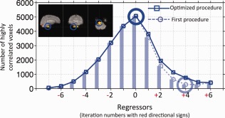
Correlation graphs of the first and optimized procedure of participant 1. Blue circle in the inlet marks the location of the single‐voxel seed from the bottom slice of the image. Correlation graph of the first procedure is plotted in shade (dotted line with small circles). Big shaded blue circle indicates the single‐voxel seed regressor (0 iteration). Correlation graph of the optimized procedure is shown as solid line with squares. Big solid blue circle indicates the optimized seed regressor. The iteration numbers with red directional signs are associated with the regressors in the optimized procedure. [Color figure can be viewed in the online issue, which is available at http://wileyonlinelibrary.com.]
The optimized procedure was developed to solve this problem. After the first recursive procedure, a second analysis starts with a new seed regressor, which is the result of averaging the most voxels selected by the previous procedure and thus represents the most accurate systemic LFOs shared by these voxels. The new seed can be regarded as resulting from a special “ROI.” The unique feature is that this spatially distributed, but temporally compact ROI is identified by the previous procedure.
Finally, we can see that the time span of the correlation graph in Figure 3 is about 5.2 s (i.e., 0.4 s × 13 = 5.2 s), which is in the range of the cerebral circulation time of healthy participants [Crandell et al., 1973; Schreiber et al., 2002].
Evolving Regressors
In Figure 4a–f, we compared the regressors (generated in Fig. 3) at 2 TR intervals. Each regressor is plotted together with the next regressor of 0.8 s shifted (in shaded lines). These maps demonstrate the great similarity between the regressors with little time difference (i.e., 0.8 s). However, the regressors are not static. In Figure 4g, the regressors of time shift 0 and 4.8 s are plotted. There is a clear difference in these two regressors with a 4.8 s time shift. The difference is the cumulative effect from the regressors' evolution over many steps that occur during this relatively long time period. This can be further demonstrated by the correlation coefficients calculated between the seed regressor and the rest of the regressors (all from the optimized procedure), as shown in Figure S1 in Supporting Information Materials. A clear decline of the correlation coefficients is observed as the regressor evolved away from the seed regressor in all participants.
Figure 4.

The regressors of participant 1 generated by the optimized procedure. Each regressor is plotted together with the next regressor of 0.8 s shift (in shaded lines) for comparison (a–f). The first and the last regressor (separated by 4.8 s) are plotted in (g). [Color figure can be viewed in the online issue, which is available at http://wileyonlinelibrary.com.]
Physiologically, the possible reasons for the evolution of the regressors are: (1) as the systemic LFOs travel with the blood though the brain, they arrive at different voxels at different times, and (2) the signal detected at each voxel is the integrated signal from all the paths of the blood flow that lead towards that point (i.e., the summation of many signals with different delay times and amplitudes). Therefore, the systemic LFO signal may vary in both time delays and amplitudes according to its location in the cerebral vasculature.
Finally, the impacts of motion on the evolving regressors have been assessed by calculating the correlation coefficients between all the regressors and six motion parameters (from FSL preprocessing) for each participant [Jenkinson et al., 2002]. The results are shown in Figure S2 in Supporting Information Material. Each graph shows the averages and standard deviations of the correlation coefficients calculated between the corresponding motion parameters (x‐axis) and all the regressors of the participant. In general, the correlation coefficients are very small (<0.1), indicating motion did not influence the regressors in this resting state study.
Dynamic Maps
Figure 5a shows the normalized z‐maps as the result of the GLM analyses according to the temporal shift in the corresponding regressor. The dynamic changes in the activation patterns represent cerebral blood flow. For example, in the sagittal view, the initial activation patterns are observed in areas densely populated with or supported by large arteries, such as polar frontal arteries, medial frontal arteries, and so forth. They gradually move towards the areas of the vascular drainage systems, such as the superior sagittal sinus and straight sinus. In the coronal view, the patterns shift from posterior cerebral arteries near superior aspects of the brain to the middle and then end in the superior sagittal sinus at top and transverse sinuses at the base of the brain. Finally, in the axial view, the pattern of activations start at the center of the cerebellum and move in two directions (anterior and posterior), ending in the transverse sinus (or Tentorial veins) and Clival venous plexus (or Jugular bulb). Arrows in the graphs of the last column of Figure 5a indicate the directions of the apparent blood flow in the corresponding orthogonal views. Figure 5b shows the participant's own phase contrast magnetic resonance angiogram (PC‐MRA) (velocity encoding factor of 30 cm/s) as a comparison, from which good matches, especially in the draining system (superior sagittal sinus, transverse sinus, etc.), were observed.
Figure 5.

Normalized z‐maps of participant 1 are displayed in sequence in orthogonal views (a). In the last graphs of each row, the movement of the patterns is pointed out by red arrows in the corresponding view. The phase contrast magnetic resonance angiogram of the same participant is shown in (b). The original z‐values (before normalization) of two example voxels (as indicated in (a)) are plotted in (c) with matching colors. [Color figure can be viewed in the online issue, which is available at http://wileyonlinelibrary.com.]
To demonstrate the utility of the normalization procedure, the z‐values of two example voxels (indicated by the blue and red arrows in Fig. 5a) from the concatenated results before normalization are shown in Figure 5c. The voxels were selected to reflect different temporal stages in the procedure (i.e., early vs. late). Voxel 1 is likely from Clival venous plexus, while voxel 2 is in the area of Posterior cerebral arteries. The traces reflect typical changes in the z‐values as a result of using the regressors of different temporal shifts. To assess the dynamic evolution, the important information (in each voxel) is the arrival time of the LFOs wave (peak position of the trace in Fig. 5c) and the duration of its passage through this voxel (width of the trace in Fig. 5c), not the z‐values themselves. In fact, the large range of the z values is probably due to the varying blood content in the voxels. This makes it difficult to display the results, and decreases the sensitivity of the dynamic map because voxels with high z‐values stay activated much longer. This issue is improved by normalizing the z‐values from each significant voxel (i.e., max z > 4). From the normalized z‐maps in Figure 5a, the activated voxels in each graph are seen to be distributed throughout the brain. This result is interesting because the temporal traces of remote voxels that are located as far away as the prefrontal cortex and posterior cerebellum can be highly correlated with the same regressor. This indicates that the LFO components of the BOLD signals from these voxels evolved roughly the same way. The LFOs are “piped” into the brain though big arteries (e.g., internal carotid artery) with no phase shift. They then follow different paths (arterioles, capillaries, etc.) as branches of the cerebral vasculature diverge. It is expected that each signal would evolve independently as it travels along its own path. The observation that some of them have evolved in a similar way, and at a the similar pace, is probably due to the uniformity in the fundamental structures of the cerebral blood system, likely reflecting the self‐invariant properties of fractal structures found throughout biological systems [Herman et al., 2001; Reishofer et al., 2012].
The blood flow patterns can be seen dynamically in the movie (top video in Supporting Information Movie S1), which shows the temporal evolution over numerous different coronal and axial views (marked by the cross on the sagittal image). The movie is shown in a 0.15 s/frame rate (a factor of 2.67 speedup) for clarity (the actual rate is 0.4 s/frame and the total time is about 5.2 s). The passage of the LFOs is clearly depicted in the movie. In addition to the passage shown in Figure 5, we also observed in axial images that the patterns started from middle areas (heavily supported by the middle cerebral arteries) to the drainage veins located at anterior and posterior of the brain (superior sagittal sinus) and the walls of the lateral ventricles.
A time delay map in which the time delays are encoded as colors is shown in Figure 6. In brief, cerebral blood flows in sequence, from earliest to latest arrival times shown in light blue, blue, red, and yellow. As a result, drainage systems are mostly colored with red and yellow, indicating they are located towards the end of the blood passage. In contrast, the areas with light blue are mostly in the top middle section of the brain fed mostly by middle cerebral arteries.
Figure 6.

Delay maps of participant 1 are shown in orthogonal views, with different colors, indicating the difference in temporal delay. [Color figure can be viewed in the online issue, which is available at http://wileyonlinelibrary.com.]
Figure 7 shows similar graphs to those presented in Figures 3 and 6 for the rest of the participants. In Figure 7a, a big blue circle marks the single‐voxel seed from the first procedure, and a big black circle marks the optimized seed. The shapes of the correlation curves are subject‐specific, resembling Gaussian or skewed Gaussian shapes. The durations are around 4–6 s. The time‐delay maps (Fig. 7b) show mostly consistent patterns as described in Figure 6. However, there are still clear differences across the participants. First, the colors, even those associated with the same structures, are different. This is mainly due to the fact that both the transit times of the LFOs and temporal delays of the seeds are different for each participant. Second, even though some main vessels (e.g., superior sagittal sinus) are commonly observed, some others (e.g., straight sinus) are not visible in all the participants. This discrepancy is probably due to the inter‐subject variations in the vasculature and cerebral blood flows. Future studies with increased spatial resolutions can be used to further investigate the causes.
Figure 7.

Correlation graphs of the rest of the participants are plotted in (a). The blue bars and the blue dotted lines indicate the correlation graphs of the first procedures, while the black lines with squares indicate the correlation graphs of the optimized procedures. Big blue and black circles mark the single seed regressors and optimized seed regressors, respectively. Delay maps of the corresponding participants are shown in (b). [Color figure can be viewed in the online issue, which is available at http://wileyonlinelibrary.com.]
Seed Selection
As we mentioned previously, the seed should be selected from the blood vessels. However, blood vessels are hard to identify from BOLD fMRI. In Materials and Methods section, we offered several suggestions to increase the likelihood of finding a “good” seed. Figures 3 and 7a show the correlation graphs of “good” seeds from all the participants. From a “good” seed, the first procedure will generate roughly 10–20 evolving regressors, mostly on one side of the seed regressor in the correction graph, covering 4–8 s (if TR = 0.4 s). The correlation graph of these regressors should resemble a Gaussian or skewed Gaussian shape. We speculate the reason to be that the correlation graph roughly indicates the volume of the region reached by the systemic LFOs in sequence. The Gaussian shaped curves (from the healthy participants) reflect to some degree the underlying vascular structure—arteries, capillaries, and veins—where the capillaries have the largest spatial distribution. However, more evidence is needed to support our hypotheses.
In every participant, the “good” seeds were all from veins (judging from the direction in which correlations with the brain were found). This is presumably because the BOLD signal is much more sensitive to the veins [Menon, 2012], and moreover, the main arteries with highly oxygenated blood (∼100%) are almost invisible to BOLD fMRI. Because of these factors, the dynamic patterns calculated from BOLD fMRI are biased towards the draining venules and veins, sampling more from venous outflow than from arterial inflow.
If a “bad” seed is chosen, three things might happen: (1) no voxel is highly correlated with the seed regressor, in which case the recursive procedure would not even start; (2) the procedure runs for a few steps before it stops (due to the threshold condition: N < 50) and the corresponding correlation graph would stay flat, with no Gaussian‐like shape produced; or (3) some regional dynamic patterns could be caught. Because a particular “bad” seed may be heavily contaminated by the regional signal, the recursive procedure may catch dynamic regional fluctuations, such as local blood circulation, and so forth. These regional dynamic fluctuations are transient and not stable. An example of a seed from the ventricle is provided in Supporting Information Figure S3, where we can see that there is a sharp spike (1.2 s duration) instead of a smooth Gaussian shape in the correlation graph.
In general, “good” seeds are fairly easy to locate using the suggestions we offered in Materials and Methods section, and the “bad” seeds should always be replaced. As we discuss in next section, because the method is very robust, many seeds, even those from non‐ideal locations, work equally well.
Robustness of the Method
Figure 8 shows the results of both the first procedure and the optimized procedure performed on participant 1 (as does Fig. 3), with four different seeds, two in gray matter (Fig. 8a,b), one in white matter (Fig. 8c), and one in the posterior cingulate cortex (Fig. 8d). The exact locations of these seeds are indicated by the blue circles in the axial images in each graph. The correlation graphs that resulted from the first procedure are plotted in red (on left), while the final correlation graphs as result of optimized procedure are plotted in blue (on right) for each seed. The correlation graph from a “good” seed (the same as that shown in Fig. 3) is also included—as “standard” (in black shaded lines)—to serve as a basis for comparison. We can observe the following from the figure:
The seeds initially chosen were not ideal. Because they were not selected from the prime locations, it is likely that they reflect relatively large contributions from the regional fluctuations, which caused a large deviation in the correlation curve (red vs. black line). This effect could influence up to three neighboring regressors.
As shown in the graphs on the left side of the figure (in red), even with these non‐ideal seeds, the recursive procedure nonetheless “corrected” them gradually, leading to an overall shape that is similar to the “standard” (black line). This demonstrates that the recursive method is robust, and able to progressively extract systemic LFOs, even if small, from these seeds and generate accurate regressors in a few steps. At the same time, given that these seeds were selected from a variety of brain regions, it implies a wide distribution of these systemic LFOs in the brain.
Also evident from the graphs on the left side of the figure (again, in red), the seeds in the correlation graph (big red circles) are in different locations relative to the whole curve. This indicates that there are temporal shifts between the systemic LFOs in these seeds due to their specific locations relative to the cerebral circulation paths, which further demonstrates the method's sensitivity to temporally shifted signals.
The good matches between the blue lines and the “standard” in the graphs on the right side of the figure indicate that the optimized procedure is effective in correcting the relatively large deviations caused by these seeds, as demonstrated by the consistency in the results regardless of the seed. In the right graphs of Figure 8c,d, small shifts were needed to match two correlation graphs (causing misaligned dots). These mismatches are caused by the temporal delay between two different initial seeds. For example, the temporal delay between two different initial seeds (from the same dataset) can be 0.2 s (not constrained by the TR). The corresponding regressors derived from these two seeds are then off by 0.2 s from each other, resulting in two correlation graphs misaligned temporally by 0.2 s. In Supporting Information Material, the corresponding video resulting from the seed in Figure 8a (Supporting Information Movie S1, at the bottom) is shown side‐by‐side with the movie generated from the seed of Figure 3 to demonstrate the consistency in the dynamic patterns.
Figure 8.

Correlation graphs of participant 1 derived from four different single‐voxel seeds (a–d). The locations of the seeds are marked by big blue circle in the axial images. The red lines on the left show the correlation graphs of the first procedures with the big red circles indicating the seed regressors. The blue lines on the right show the correlation graphs of the optimized procedures. In all the graphs, shaded black lines show the correlation graphs derived from a “good” seed (as shown in Fig. 3). [Color figure can be viewed in the online issue, which is available at http://wileyonlinelibrary.com.]
We used the short TR in this study, which had several benefits. First, the TR determines the time resolution of the dynamic map (TR = evolving step in time). The cerebral circulation time of cerebral blood flow is about 4–7 s [Crandell et al., 1973; Ibaraki et al., 2007; Schreiber et al., 2002], as shown in Figure 3. With a TR value of 2 or 3 s, only two to four time points can be generated, which dramatically reduces the resolution in dynamic maps. However, due to the low frequency (∼0.1 Hz) of the blood signal we tracked, the BOLD signal with longer TR (2–3 s) should have enough information. Therefore, we can oversample the BOLD signal of long TRs (e.g., 2 s) with much smaller TRs (e.g., 400 ms) to increase the time resolution and then apply the method to the new data to calculate the dynamic map. We have tested this strategy on other resting state data with longer TR (=1.5 s) and were able to successfully map out similar flow patterns (see Supporting Information Movie S2), which further demonstrates the robustness of the method and greatly broadens its applications. Another benefit of using short TR is that it allows other physiological noise arising from respiratory and cardiac signals to be fully sampled and then filtered out of the data, thereby conferring more accurate results. To summarize the main thrust of these points: although using the short TR is not necessary for the objective of tracking LFOs, doing so leads to greater accuracy in the results obtained.
Finally, we show in Figure S4 in Supporting Information Material the four dynamic patterns side‐by‐side, which were derived from different temporal sections of a long study (600 s). In general, the dynamic patterns are stable among these results, and similar numbers of recursive steps were automatically generated. However, there are some visible differences in the pattern. There are a few possible explanations for these discrepancies. First, when calculating the voxel‐wise cross correlation, the resulting coefficients reflect the average values over the length of the temporal traces used. Therefore, the resulting flow map does not correspond to one particular time point; rather, it is the averaged result of the entire systemic LFOs' duration. For example, the results in Figure S4 of Supporting Information material reflect the averaged flow patterns of the 600 s, first 200 s, middle 200 s, and last 200 s, respectively. As we know, the flow patterns are dynamic even in resting states. This is why the result from the first 200 s is similar to that from the middle 200 s, albeit with subtle differences. Another factor is that the results from shorter duration scans are more prone to physiological noise. Sporadic motion artifacts happening in the first 200 s, for example, would significantly affect the results of that section, but not the other sections. In addition, the effect of sporadic motion on the whole timecourse (600 s) is smaller because long runs tend to average out the sporadic noise.
Applications
Figures 6 and 7b show the delay maps for each participant. We can see that most of the voxels are highly correlated with the systemic LFOs at certain time shifts, indicated by the color. This correlation demonstrates that the majority of the voxels are affected by these systemic LFOs, especially in resting state studies, in which the neuronal signal is relatively small. Most current denoising methods use static or temporally shifted static noise regressors [Birn et al., 2008; Carbonell et al., 2011; Chang et al., 2009; Frederick et al., 2012]. However, as we now know, the systemic LFOs evolve, a phenomenon that is clearly demonstrated in Supporting Information Figures S4 and S1. Using static noise regressors may not thoroughly remove these changing systemic LFOs. The evolving regressors, however, can be used to remove this dynamic noise more efficiently, increasing the sensitivity in detecting neuronal BOLD signals. Furthermore, we found that some resting state networks were affected by these systemic LFOs [Tong et al., 2013] in a certain sequence that matched the blood flow. This finding indicates that the signals from these networks could be greatly influenced by the various temporal shifts of the LFOs. We believe that the method tested in this study can be used to effectively identify the non‐neuronal LFOs and, thus, dramatically improve both the SNR for BOLD data, and the accuracy of RSN detection and quantification.
A major benefit of this method is that it is an automatic, data driven procedure; aside from selecting the seed voxel, no additional measurements or interventions are needed. Moreover, the information on cerebral flow is calculated using ordinary BOLD fMRI data; no special MRI sequence is required. Therefore, the method we propose can be applied to any future or existing resting state studies. On top of the resting state results, the method also provides additional valuable information about the cerebral blood flow at no cost. This could become extremely useful for studies on aging populations, stroke, Alzheimer's disease, and so forth, which are known to affect the cerebral vasculature. It can also be modified to track regional blood flow changes caused by task activations. The modified version is currently being developed and tested on data from visual stimulations.
The method offers several advantages over perfusion MRI using exogenous contrast agent (e.g., DSC MRI), the most significant drawbacks of which are invasiveness and potential toxicity of the contrast agent. These features of perfusion MRI necessitate careful subject screening and monitoring before and during the procedure [Knutsson et al., 2010]. First, this method is pure analytical and can be widely applied to nearly all the fMRI data. Second, it offers whole brain coverage. Finally, it can roughly assess the direction and duration of the flow through out brain. As the method uses fMRI data, its temporal and spatial resolution are decided by those of BOLD signal. Normally, they are lower than those of DSC MRI. However, they can be greatly improved by multiband sequence (which can be used to increase either the temporal or the spatial resolution significantly).
Limitations
Although the method is very promising and the procedure is already robust, there are several areas in need of improvement at this early stage. First and foremost is to validate the method. The movement of LFOs in the brain resembles the cerebral blood flow by its dynamic patterns and duration. To date, we have conducted phase contrast angiographic MRI on two participants, and our results further confirm that the voxels highlighted by this procedure match the major vessels of the brain (primarily the veins). At the time of writing, we are commencing a follow‐up study with other quantitative MR flow methodologies—specifically, dynamic susceptibility contrast (DSC MRI) and ASL—to further validate this method.
Because the origin and function of the LFO signal remain unclear [Sassaroli et al., 2012; Tanaka et al., 2006; Wise et al., 2004; Zuo et al., 2010], its spectral range is not well‐defined. In addition, the neuronal activation measured by BOLD fMRI is in a similar spectral band, which makes it hard to isolate systemic LFOs in the brain. In our previous research, we used NIRS to measure the LFOs in the periphery (i.e., finger and toe) while participants underwent fMRI scanning. We found the LFOs (i.e., Δ[tHb]) measured at finger (or toe) were highly correlated with many BOLD signals in the brain, with a time shift [Tong et al., 2012], which confirms that the LFOs are systemic. We further explored the spectral feature of these LFOs by correlating only the signals from the finger and those from the toe (neither has neuronal signals). The highest correlations were found between the spectral range 0.05–0.2 Hz (unpublished data), which was the range used in this study. Obviously, more studies are needed for a full understanding of the systemic LFOs and their spectral features, and there is likely to be variation between individual subjects. For this study, however, the rough range chosen was sufficient and effective in producing the dynamic maps.
The whole process is not fully automatic. First, the initial seed selection is manual. It relies on the researcher to identify the seed from big blood vessels. However, there are several existing data‐driven fMRI methods which could help to automate the step using principal component analysis [Behzadi et al., 2007], spatial independent component analysis [Perlbarg et al., 2007], amplitude of LFOs analysis [Zou et al., 2008], and canonical autocorrelation analysis [Churchill and Strother, 2013] to identify physiological regions and their corresponding temporal traces. We will evaluate these methods for incorporation into our method. Second, to terminate the recursive procedure, we selected an empirical threshold (i.e., 50; as discussed in Recursive Regressors section). However, sometimes, it failed to terminate the procedure before the number of voxels selected (i.e., N) increased again. This is probably due to the pseudo‐periodic feature of the LFOs signals. For example, the periodic signal of LFOs (∼0.1 Hz) is oscillating approximately every 10 s. In that case, we have to monitor the number of highly correlated voxels in the correlation graph (such as Fig. 3 and 7a) closely. If the number starts to increase again after it reaches the minimum, we will stop it manually.
CONCLUSION
The present report describes a recursive procedure to extract the evolving systemic LFOs from BOLD fMRI and how it can be used to dynamically map cerebral blood flow. We have shown that the dynamic patterns—derived by application of our method to resting state data from seven healthy participants—resemble cerebral blood flow with respect to both paths of flow and cerebral circulation times. The utility of our method is likely to be particularly attractive for researchers interested in cerebral blood circulation changes during functional studies, as it does not require special MR acquisition parameters or exogenous contrast agents. Thus, the cerebrovascular information detailed above can be extracted from typical fMRI datasets in parallel with functional analyses. Moreover, this study demonstrates the evolution of the systemic LFOs and an effective way to extract them, a capability which will dramatically improve the denoising procedure used in fMRI to reveal the actual neuronal signals in the BOLD.
Supporting information
Supplementary Information Figure 1.
Supplementary Information Figure 2.
Supplementary Information Figure 3.
Supplementary Information Figure 4.
Supplementary Information Movie 1.
Supplementary Information Movie 2.
ACKNOWLEDGMENTS
The authors thank Dr. Scott Lukas for his support on the project and helpful discussions. The authors thank Drs. Kim Lindsey, Amy Janes, Lia Hocke, and Carolyn Caine for their comments. The authors also want to thank the reviewers for their valuable comments, which helped to improve the quality of this manuscript considerably.
REFERENCES
- Aalkjaer C, Boedtkjer D, Matchkov V (2011): Vasomotion—What is currently thought? Acta Physiol (Oxf) 202:253–269. [DOI] [PubMed] [Google Scholar]
- Allen J, Murray A (2003): Age‐related changes in the characteristics of the photoplethysmographic pulse shape at various body sites. Physiol Meas 24:297–307. [DOI] [PubMed] [Google Scholar]
- Bandettini PA, Wong EC, Hinks RS, Tikofsky RS, Hyde JS (1992): Time course EPI of human brain function during task activation. Magn Reson Med 25:390–397. [DOI] [PubMed] [Google Scholar]
- Behzadi Y, Restom K, Liau J, Liu TT (2007): A component based noise correction method (CompCor) for BOLD and perfusion based fMRI. NeuroImage 37:90–101. [DOI] [PMC free article] [PubMed] [Google Scholar]
- Bhattacharyya PK, Lowe MJ (2004): Cardiac‐induced physiologic noise in tissue is a direct observation of cardiac‐induced fluctuations. Magn Reson Imaging 22:9–13. [DOI] [PubMed] [Google Scholar]
- Birn RM, Smith MA, Jones TB, Bandettini PA (2008): The respiration response function: The temporal dynamics of fMRI signal fluctuations related to changes in respiration. NeuroImage 40:644–654. [DOI] [PMC free article] [PubMed] [Google Scholar]
- Buxton RB (2002): Introduction to Functional Magnetic Resonance Imaging: Principles and Techniques. Cambridge, UK: Cambridge University Press. [Google Scholar]
- Carbonell F, Bellec P, Shmuel A (2011): Global and system‐specific resting‐state fMRI fluctuations are uncorrelated: principal component analysis reveals anti‐correlated networks. Brain Connect 1:496–510. [DOI] [PMC free article] [PubMed] [Google Scholar]
- Chang C, Cunningham JP, Glover GH (2009): Influence of heart rate on the BOLD signal: The cardiac response function. NeuroImage 44:857–869. [DOI] [PMC free article] [PubMed] [Google Scholar]
- Churchill NW, Strother SC (2013): PHYCAA+: An optimized, adaptive procedure for measuring and controlling physiological noise in BOLD fMRI. NeuroImage 82:306–325. [DOI] [PubMed] [Google Scholar]
- Cordes D, Haughton VM, Arfanakis K, Carew JD, Turski PA, Moritz CH, Quigley MA, Meyerand ME (2001): Frequencies contributing to functional connectivity in the cerebral cortex in “resting‐state” data. AJNR Am J Neuroradiol 22:1326–1333. [PMC free article] [PubMed] [Google Scholar]
- Crandell D, Moinuddin M, Fields M, Friedman BI, Robertson J (1973): Cerebral transit time of 99m technetium sodium pertechnetate before and after cerebral arteriography. J Neurosurg 38:545–547. [DOI] [PubMed] [Google Scholar]
- D'Esposito M, Deouell LY, Gazzaley A (2003): Alterations in the BOLD fMRI signal with ageing and disease: a challenge for neuroimaging. Nat Rev Neurosci, 4:863–872. [DOI] [PubMed] [Google Scholar]
- Feinberg DA, Moeller S, Smith SM, Auerbach E, Ramanna S, Gunther M, Glasser MF, Miller KL, Ugurbil K, Yacoub E (2010): Multiplexed echo planar imaging for sub‐second whole brain FMRI and fast diffusion imaging. PLoS One 5:e15710. [DOI] [PMC free article] [PubMed] [Google Scholar]
- Frederick B, Nickerson LD, Tong Y (2012): Physiological denoising of BOLD fMRI data using Regressor Interpolation at Progressive Time Delays (RIPTiDe) processing of concurrent fMRI and near‐infrared spectroscopy (NIRS) NeuroImage 60:1913–1923. [DOI] [PMC free article] [PubMed] [Google Scholar]
- Herman P, Kocsis L, Eke A (2001): Fractal branching pattern in the pial vasculature in the cat. J Cereb Blood Flow Metab 21:741–753. [DOI] [PubMed] [Google Scholar]
- Huettel SA, Song AW, McCarthy G (2009): Functional Magnetic Resonance Imaging. Sunderland, MA: Sinauer Associates, Incorporated. [Google Scholar]
- Ibaraki M, Ito H, Shimosegawa E, Toyoshima H, Ishigame K, Takahashi K, Kanno I, Miura S (2007): Cerebral vascular mean transit time in healthy humans: A comparative study with PET and dynamic susceptibility contrast‐enhanced MRI. J Cereb Blood Flow Metab 27:404–413. [DOI] [PubMed] [Google Scholar]
- Jenkinson M, Bannister P, Brady M, Smith S (2002): Improved optimization for the robust and accurate linear registration and motion correction of brain images. NeuroImage 17:825–841. [DOI] [PubMed] [Google Scholar]
- Jenkinson M, Beckmann CF, Behrens TE, Woolrich MW, Smith SM (2012): Fsl. NeuroImage 62:782–790. [DOI] [PubMed] [Google Scholar]
- Julien C (2006): The enigma of Mayer waves: Facts and models. Cardiovasc Res 70:12–21. [DOI] [PubMed] [Google Scholar]
- Knutsson L, Stahlberg F, Wirestam R (2010): Absolute quantification of perfusion using dynamic susceptibility contrast MRI: Pitfalls and possibilities. MAGMA 23:1–21. [DOI] [PubMed] [Google Scholar]
- Leopold DA, Maier A (2012): Ongoing physiological processes in the cerebral cortex. NeuroImage 62:2190–2200. [DOI] [PMC free article] [PubMed] [Google Scholar]
- Menon RS (2012): The great brain versus vein debate. NeuroImage 62:970–974. [DOI] [PubMed] [Google Scholar]
- Murphy K, Birn RM, Bandettini PA (2013): Resting‐state fMRI confounds and cleanup. NeuroImage 80:349–359. [DOI] [PMC free article] [PubMed] [Google Scholar]
- Murphy K, Harris AD, Wise RG (2011): Robustly measuring vascular reactivity differences with breath‐hold: Normalising stimulus‐evoked and resting state BOLD fMRI data. NeuroImage 54:369–379. [DOI] [PubMed] [Google Scholar]
- Ogawa S, Tank DW, Menon R, Ellermann JM, Kim SG, Merkle H, Ugurbil K (1992): Intrinsic signal changes accompanying sensory stimulation: Functional brain mapping with magnetic resonance imaging. Proc Natl Acad Sci USA 89:5951–5955. [DOI] [PMC free article] [PubMed] [Google Scholar]
- Perlbarg V, Bellec P, Anton JL, Pelegrini‐Issac M, Doyon J, Benali H (2007): CORSICA: Correction of structured noise in fMRI by automatic identification of ICA components. Magn Reson Imaging 25:35–46. [DOI] [PubMed] [Google Scholar]
- Reishofer G, Koschutnig K, Enzinger C, Ebner F, Ahammer H (2012): Fractal dimension and vessel complexity in patients with cerebral arteriovenous malformations. PLoS One 7:e41148. [DOI] [PMC free article] [PubMed] [Google Scholar]
- Sassaroli A, Pierro M, Bergethon PR, Fantini S (2012): Low‐frequency spontaneous oscillations of cerebral hemodynamics investigated with near‐infrared spectroscopy: A review. IEEE J Sel Top Quantum Electron 18:1478–1492. [Google Scholar]
- Scholvinck ML, Maier A, Ye FQ, Duyn JH, Leopold DA (2010): Neural basis of global resting‐state fMRI activity. Proc Natl Acad Sci USA 107:10238–10243. [DOI] [PMC free article] [PubMed] [Google Scholar]
- Schreiber SJ, Franke U, Doepp F, Staccioli E, Uludag K, Valdueza JM (2002): Dopplersonographic measurement of global cerebral circulation time using echo contrast‐enhanced ultrasound in normal individuals and patients with arteriovenous malformations. Ultrasound Med Biol 28:453–458. [DOI] [PubMed] [Google Scholar]
- Shmueli K, van Gelderen P, de Zwart JA, Horovitz SG, Fukunaga M, Jansma JM, Duyn JH (2007): Low‐frequency fluctuations in the cardiac rate as a source of variance in the resting‐state fMRI BOLD signal. NeuroImage 38:306–320. [DOI] [PMC free article] [PubMed] [Google Scholar]
- Smith SM, Jenkinson M, Woolrich MW, Beckmann CF, Behrens TE, Johansen‐Berg H, Bannister PR, De Luca M, Drobnjak I, Flitney DE, Niazy RK, Saunders J, Vickers J, Zhang Y, De Stefano N, Brady JM, Matthews PM (2004): Advances in functional and structural MR image analysis and implementation as FSL. NeuroImage 23 Suppl 1:S208–219. [DOI] [PubMed] [Google Scholar]
- Tanaka Y, Nariai T, Nagaoka T, Akimoto H, Ishiwata K, Ishii K, Matsushima Y, Ohno K (2006): Quantitative evaluation of cerebral hemodynamics in patients with moyamoya disease by dynamic susceptibility contrast magnetic resonance imaging—Comparison with positron emission tomography. J Cereb Blood Flow Metab 26:291–300. [DOI] [PubMed] [Google Scholar]
- Tong Y, Frederick BD (2010): Time lag dependent multimodal processing of concurrent fMRI and near‐infrared spectroscopy (NIRS) data suggests a global circulatory origin for low‐frequency oscillation signals in human brain. NeuroImage 53:553–564. [DOI] [PMC free article] [PubMed] [Google Scholar]
- Tong Y, Hocke LM, Licata SC, Frederick B (2012): Low‐frequency oscillations measured in the periphery with near‐infrared spectroscopy are strongly correlated with blood oxygen level‐dependent functional magnetic resonance imaging signals. J Biomed Opt 17:106004. [DOI] [PMC free article] [PubMed] [Google Scholar]
- Tong Y, Hocke LM, Nickerson LD, Licata SC, Lindsey KP, Frederick B (2013): Evaluating the effects of systemic low frequency oscillations measured in the periphery on the independent component analysis results of resting state networks. NeuroImage 76:202–215. [DOI] [PMC free article] [PubMed] [Google Scholar]
- Tong Y, Lindsey KP, Frederick BD (2011): Partitioning of physiological noise signals in the brain with concurrent near‐infrared spectroscopy and fMRI. J Cereb Blood Flow Metab 31:2352–2362. [DOI] [PMC free article] [PubMed] [Google Scholar]
- Wise RG, Ide K, Poulin MJ, Tracey I (2004): Resting fluctuations in arterial carbon dioxide induce significant low frequency variations in BOLD signal. NeuroImage 21:1652–1664. [DOI] [PubMed] [Google Scholar]
- Zou QH, Zhu CZ, Yang Y, Zuo XN, Long XY, Cao QJ, Wang YF, Zang YF (2008): An improved approach to detection of amplitude of low‐frequency fluctuation (ALFF) for resting‐state fMRI: Fractional ALFF. J Neurosci Methods 172:137–141. [DOI] [PMC free article] [PubMed] [Google Scholar]
- Zuo XN, Di Martino A, Kelly C, Shehzad ZE, Gee DG, Klein DF, Castellanos FX, Biswal BB, Milham MP (2010): The oscillating brain: Complex and reliable. NeuroImage 49:1432–1445. [DOI] [PMC free article] [PubMed] [Google Scholar]
Associated Data
This section collects any data citations, data availability statements, or supplementary materials included in this article.
Supplementary Materials
Supplementary Information Figure 1.
Supplementary Information Figure 2.
Supplementary Information Figure 3.
Supplementary Information Figure 4.
Supplementary Information Movie 1.
Supplementary Information Movie 2.