Iterative CT Reconstruction using Models of Source and Detector Blur and Correlated Noise

Abstract

Statistical model-based reconstruction methods derive much of their advantage over traditional methods through more accurate forward models of the imaging system. Typical forward models fail to integrate two important aspects of real imaging systems: system blur and noise correlations in the measurements. This work develops an approach that models both aspects using a two-stage approach that includes a regularization deblurring operation followed by generalized penalized weighted least-squares reconstruction. Different reconstruction noise models including standard uncorrelated and correlated presumptions were explored. Moreover, different imaging systems were investigated in which blur was dominated by source effects, dominated by detector effects, or by a combination of source and detector blur. The proposed reconstruction approach that models the correlated noise demonstrated the best performance across all scenarios with the greatest benefits for increased source blur and for reconstructions with finer spatial resolution. This suggests potential application of the method for high resolution systems like dedicated flat-panel cone-beam CT (e.g., head, extremity, dental, mammography scanners) where system resolution is limited by both source and detector blur effects and noise correlations in measurement data are traditionally ignored.

I. INTRODUCTION

Model-based tomographic reconstruction techniques have demonstrated better dose utilization and noise versus image quality tradeoff than traditional methods [1]. Such advantages are, in part, due to the integration of improved forward models that more accurately represent the physics and noise processes of acquisition and detection. Forward models of varying complexity can be designed to incorporate different imaging system characteristics, such as source and detector blur [2][3]. While recent studies [4] suggest that blur modeling may not yield substantial improvements for current diagnostic CT scanners and scan protocols, the advantages of blur modeling are dependent on target spatial resolutions and system geometries. For example, degradations in spatial resolution are potentially much more important in systems like dedicated flat-panel cone-beam CT that has been developed for high spatial resolution applications (e.g., temporal bone, extremity, dental imaging). The intrinsic spatial resolution in these systems is limited by both detector and source blurring effects. Detector blur tends to be dominated by light spread in the scintillator as opposed to detector aperture effects, since the pixel size tends to be small compared to the scintillator blur. Source blur is also often more pronounced in such systems due to the compact geometries (short source-to-detector distances) and the use of fixed anode sources with focal spots that are larger than their rotating anode counterparts.

Thus, higher fidelity forward models like those in [2][3] that incorporate system blur offer an opportunity to recover lost spatial resolution. However, those approaches and nearly all traditional model-based reconstruction methods make an important assumption about the underlying noise model that is potentially quite inaccurate for flat-panel systems that use indirect detection. Specifically, the conversion of primary quanta to secondary quanta in the scintillator of an indirect detector imparts spatial correlations in the measurement noise. These correlations are visibly evident in gain scan acquisitions, yet the standard assumption for statistical model-based reconstruction is to presume that the measurements are independent. Despite this noise model mismatch, model-based approaches have demonstrated an advantage in cone-beam CT [1]. However, we hypothesize that additional advantages can be attained when more accurate noise modeling is integrated in the reconstruction, particularly in high spatial resolution applications in which system blur is also modeled.

Previous work [5] has shown that integrating a correlated noise model into the reconstruction process allows for improved tradeoffs between noise and resolution. In [5], a linearization of the data that included a deblurring operation followed by penalized generalized weighted least-squares reconstruction was introduced and applied to an imaging system with equal amounts of source and detector blur. The work presented here further generalizes the methodology of [5] to consider regularized deblurring of projection data and extends the investigations to systems with varying degrees of source and detector blur. Specifically, we consider scenarios where source blur is dominated by source effects, or dominated by detector effects, or is a mixture of source and detector effects to find where blur and correlated noise modeling yields the greatest advantage. Understanding this relationship has important implications for hardware design in cone-beam CT systems, including choices in the system geometry, focal spot size, scintillator thickness, etc.

In the following sections, the generalized reconstruction approach with system blur and a correlated noise model is introduced and investigated. Three different noise models - white noise, uncorrelated noise with unequal variances, and generalized correlated noise - are compared in simulated CT studies, and the improved performance using the correlated noise model is demonstrated

II. METHODS

A. Forward Model and Correlated Noise Model

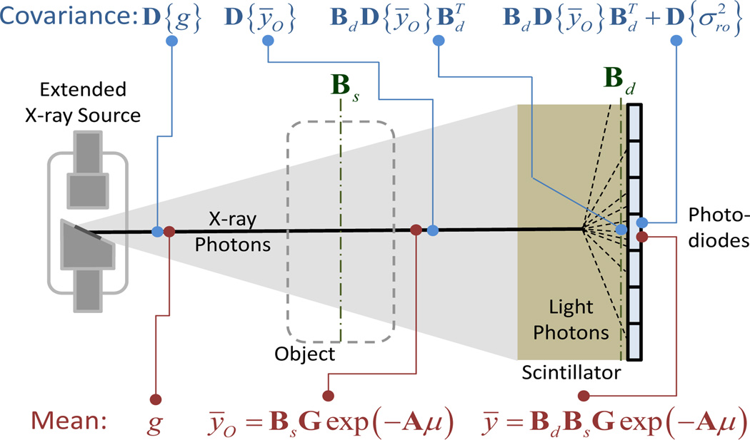
The system model for a general CT system with indirect detection is illustrated in Figure 1. The mean measurement model that we adopt for development of the reconstruction algorithm has the following form:

$$\overline{y}={\mathbf{B}}_d{\mathbf{B}}_s\mathbf{G}\text{exp}(-\mathbf{A}\mu )\mathbf{G}=\mathbf{D}\left\{g\right\}$$ (1)

which uses a monoenergetic formulation of Beer's law where the image volume is denoted by μ, the projection operation is represented by the system matrix A, and the diagonal matrix G denotes a gain associated with each detector ray (i.e. x-ray fluence). (The notation D{·} denotes the operator that puts the vector operand onto the diagonal elements of a diagonal matrix.) Two linear blur operators are included that model the effects of source blur, B_sand detector blur B_d separately. This model is an approximation, particularly for source blur, since source effects are depth-dependent. However, for objects that are relatively thin (without a substantial change in magnification across the volume) this is a convenient and reasonable approximation.

Fig. 1.

System model for a generalized indirect detector cone-beam CT system. Following the generation and transit of photons (left to right), the mean number of quanta and the covariance associated with those quanta are modeled. Specifically, the mean distribution of x-ray photons at generation (g) is both attenuated by the object and undergoes spatial blurring due to the extended source. In the detector, additional blur due to light spread in the scintillator is modeled yielding the form for the mean measurement model. Noise undergoes a similar propagation through the system starting with independent photon noise with variance equal to the mean. Changes in the mean due to attenuation in the object modify these variances, which then exhibit spatial spreading (correlation) in the scintillator. Finally, these correlated measurements may be modified with the addition of (independent) readout noise.

The propagation of noise through the imaging system is also illustrated in Figure 1. Photons generated at the x-ray source are presumed to be independent with a variance equal to their mean (e.g., a Gaussian approximation to a Poisson distribution) yielding a diagonal covariance matrix. Some x-ray photons are attenuated in the object modifying these variances by their survival probabilities as well as spatial spreading due to source blur; however, the noise remains uncorrelated at this point. In the detector, individual x-ray photons are converted to many light photons, which spread spatially (detector blur) and correlate the noise. Lastly, photodiodes convert light photons to a digital signal with possible readout noise (presumed independent and Gaussian with standard deviation equal to σ_ro). This results in the following model for the distribution of noise in the measurements:

$$y~\text{Gaussian}(\overline{y},{\mathbf{K}}_y){\mathbf{K}}_y={\mathbf{B}}_d{\mathbf{K}}_q{\mathbf{B}}_d^T+{\mathbf{K}}_r{\mathbf{K}}_d=\mathbf{D}\left\{{\sigma }_{\mathit{\text{quantum}}}^2\right\}=\mathbf{D}\left\{{\overline{y}}_o\right\}{\mathbf{K}}_r=\mathbf{D}\left\{{\sigma }_{ro}^2\right\}$$ (2)

with the following covariance matrices: K_q represents predetection uncorrelated quantum noise, K_r denotes uncorrelated readout noise, and K_y is the covariance associated with the measurement vector y.

As in [5], rather than trying to solve the generalized nonlinear least-squares reconstruction problem, we choose to transform the measurements to obtain a linear least-squares objective function. Specifically, we may compute estimated line integrals using the follow equation

$$\widehat{l}(y)=-\text{log}({\mathbf{G}}^{-1}{\mathbf{B}}^{-1}y).$$ (3)

This transformation includes the familiar normalization (G⁻¹) and logarithm operations, but also includes a deblurring of projection data represented by B⁻¹.

Ideally, this deblurring would remove spatial resolution losses associated with both the source and detector blur suggesting that

$${\mathbf{B}}^{-1}\approx {[{\mathbf{B}}_d{\mathbf{B}}_s]}^{-1}$$ (4)

Unfortunately, such an inverse may not exist, or the inverse is highly ill-conditioned, yielding computational difficulties and potential noise amplification. Instead, we adopt the following regularized pseudo-inverse

$${\mathbf{B}}^{-1}={[{\mathbf{B}}_s^T{\mathbf{B}}_d^T{\mathbf{B}}_d{\mathbf{B}}_s+\lambda \mathbf{I}]}^{-1}{\mathbf{B}}_s^T{\mathbf{B}}_d^T.$$ (5)

This transformation allows for regularized inversion of the source and detector blurs and includes a parameter λ to control the strength of the regularization. (Here, we have adopted a magnitude regularization scheme, but other options, including pairwise roughness penalties, could also be applied.)

Applying the linearization in (3) suggests the following generalized penalized weighted (linear) least-squares reconstruction objective function:

$$\widehat{\mu }=\text{argmin}{\Vert \widehat{l}(y)-\mathbf{A}\mu \Vert }_{{\mathbf{K}}_l^{-1}}^2+\beta R(\mu )={[{\mathbf{A}}^T{\mathbf{K}}_l^{-1}\mathbf{A}+\beta {\mathbf{R}}_{\mu }]}^{-1}{\mathbf{A}}^T{\mathbf{K}}_l^{-1}\widehat{l}(y).$$ (6)

which encourages a fit between the line integral estimates and the projected image volume estimate. In this case, we have adopted a quadratic regularization term which leads to a closed form solution with penalty strength governed by the scalar parameter β. Central to the data fitting is a weighting by the inverse of the covariance associated with the estimated line integrals. Thus, an expression K_l is required. As in [5], propagating the measurement covariance K_y through the transformation in (3), one can show that the covariance of the line integral estimates may be approximated as

$${\mathit{K}}_l\approx \mathit{D}\left\{\frac{1}{{\mathit{B}}^{-1}\overline{y}}\right\}{\mathit{B}}^{-1}{\mathit{K}}_y{[{\mathit{B}}^{-1}]}^T\mathit{D}\left\{\frac{1}{{\mathit{B}}^{-1}\overline{y}}\right\}$$ (7)

While the estimator in (6) is fully specified with the definitions in (5) and (7), there are a number of practical concerns in performing this optimization.

B. Practical Implementation

For typical CT systems, it is impractical to store and invert most of the matrices defined above. Thus, the action of the matrices is implemented functionally. This includes projection and backprojection functions, shift-invariant blur functions implemented using Fourier methods, and computation of K_l through serial application of each of its components. The measured data were used as an approximation for ȳ in (7), and K_q in (2) was approximated from measurements by D{B⁻¹y}.

The matrix inverses require special treatment as well. For shift-invariant blur functions, (5) may be computed directly using Fourier domain division. The action of the remaining three matrix inverses in (6) are computed using conjugate gradient (CG) based approximation.

Noting that (6) can be rewritten as

$$\mathit{S}\widehat{\mu }=b$$ (8)

$$b={\mathit{A}}^T{\mathit{K}}_l^{-1}\widehat{l}(y)$$ (9)

$$\mathit{S}={\mathit{A}}^T{\mathit{K}}_l^{-1}\mathit{A}+\beta {\mathit{R}}_{\mu }$$ (10)

we see that the inverse in (9) can be approximated with one CG loop, whereas approximating (8) requires a nested loop with an inner CG loop to estimate the inverse in (10) and an outer CG loop to solve (8).

In this work, the inner loop K_l inversions in (10) were performed using a maximum of 100 CG iterations, and the outer loop inversion in (8) used a maximum of 250 CG iterations. The inversion in (9) used a maximum 1000 CG updates. All optimization code was written in Python with calls to external GPU libraries for fast projection and backprojection operations.

C. Simulation Experiments

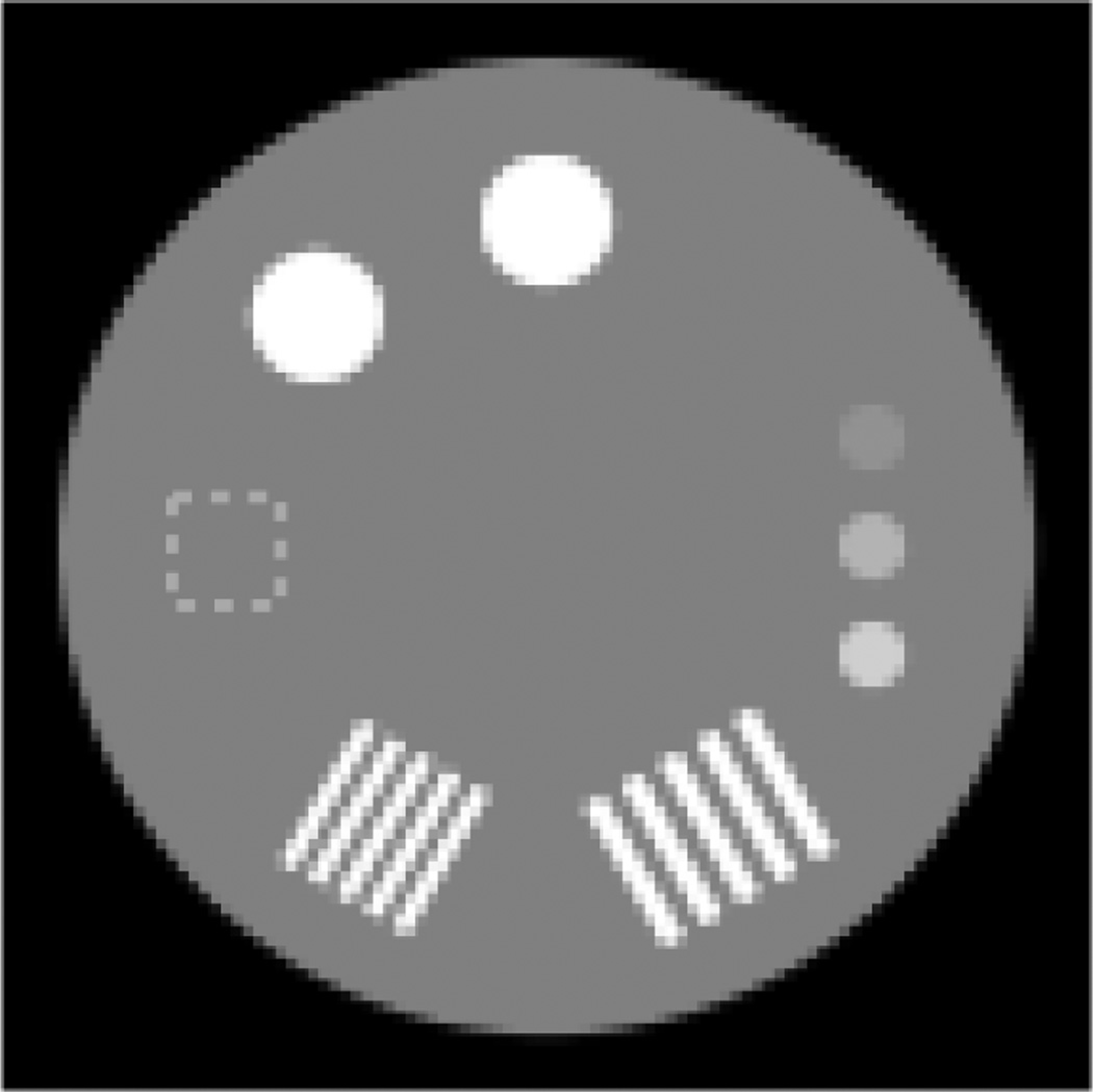
To investigate the performance of the proposed reconstruction approach, simulation experiments were conducted using the phantom in Figure 2. The system geometry used a 100x100 axial image reconstruction with 0.1 mm voxels and a 1D detector array of 150 pixels with 0.14 mm pitch. The source-to-detector distance was 400 mm and source-to-axis distance was 200 mm. Projection data were obtained for 360 angles over 360°. Predetection quantum noise was simulated using a Gaussian distribution with a constant 10⁵ photons in the unattenuated beam (with variance equal to mean). For these initial studies, readout noise variance was set to 0.

Fig. 2.

Two-dimensional digital phantom used for performance investigations. The phantom comprises low and high-contrast targets and two sets of line pairs. A square region of interest in a uniform region of the phantom is indicated with a dashed line showing where variance in the reconstructed image is computed.

We compared reconstructions using the generalized penalized weighted least-squares approach of (6) using three different noise models: 1) The correlated noise model described in (7); 2) a white Gaussian noise model; and 3) an uncorrelated Gaussian model that presumed each measurement had a variance equal to its mean (approximating a Poisson random variable). Additionally, we consider three different blur scenarios with Gaussian source and detector blurs. Specifically, three imaging systems were modeled with: 1) detector dominated blur (2.121 pixels FWHM detector, 0.001 pixels FWHM source blur); 2) equally distributed blur, (1.5 pixels FWHM source and detector blur); and 3) source dominated blur (0.001 pixels FWHM detector, 2.121 pixels FWHM source blur). We performed a dual parameter sweep (β and λ) for each noise model and blur scenario combination.

To compare images, bias and variance were calculated for each reconstruction. Bias was calculated using a reconstruction of noiseless data according to the following:

$$\mathit{\text{bias}}={\left|\right|{\widehat{\mu }}_{\mathit{\text{noiseless}}}-{\mu }_{\mathit{\text{true}}}\left|\right|}^2$$ (11)

The variance was calculated as the spatial variance over a flat part of a reconstruction (indicated with dashed line in Fig. 2).

III. RESULTS

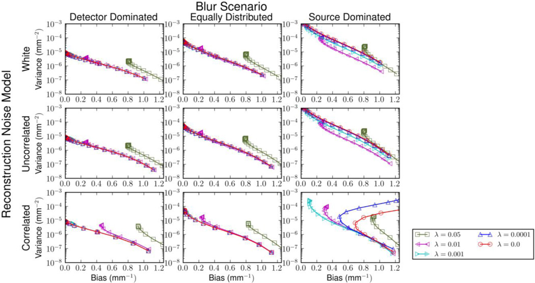
Fig. 3. shows plots of bias versus variance for each of the reconstruction noise models and each of the three different blur scenarios. In particular this investigation shows the relative performance of different methods across a wide range of regularization strengths for the deblurring operation (λ) and for reconstruction (β ). Within each plot of Fig. 3 there are five curves representing the bias versus variance performance for a fixed value of λ and varying β. In the case of detector dominated blur, there was little or no benefit from using a regularized de-blur. It appears that the added bias due to increased λ did not improve the noise tradeoff, and the added bias becomes a detriment at higher values of λ.

Fig. 3.

Plots of bias versus variance for the three noise models of reconstruction and the three system blur scenarios. The plots contain a summary of results from the two-dimensional parameter sweep over λ and β. Within each plot five separate curves for fixed λ are shown. Individual curves are generated by sweeps over β. The importance of regularization in the deblurring step is most important in the source dominated scenario where nonzero λ values improve the bias-variance relationship for each reconstruction noise model.

Similar trends are evident in the case of equal source and detector blurs. That is, the regularization in the deblurring step does not appear to improve the bias-variance tradeoff and at higher λ, this added regularization is detrimental.

The situation is different for the case of source dominated blur. In this case, increased regularization in the deblurring step improves the bias-variance tradeoff. However, the relationship is more complex and depends on the noise model in the reconstruction. For the white noise and uncorrelated noise models, λ=0.01 is optimal over much of the bias range; however, the optimal λ decreases at lower bias levels (as induced by small β values). For the correlated noise model, there appears to be a single optimal λ value over the range with λ=0.001. The correlated noise plots also show unusual behavior for very low β values when λ is also low. Specifically, lower β appear to increase bias. This is likely due to ringing in the reconstruction for (nearly) unregularized solutions.

To compare the three noise models with each other, we consolidated the above sweeps into a single curve for each noise model by selecting the (λ,β) pair that achieves the best performance for each bias level. These results are summarized in Fig. 4.

Fig. 4.

Bias-variance plots for each blur scenario with optimal selection of (λ,β). These plots illustrate the relative performance of each reconstruction noise model. In the detector blur dominated scenario, the three models perform comparably. In both the equal blur and source dominated blur scenarios, the correlated noise model shows the best performance and the white noise model shows the worst performance. The relative gain of the correlated noise model is greatest in the source blur dominated scenario.

When the blur is dominated by the detector, the overall image quality is better than the other blur scenarios, and the three noise models perform similarly. Equivalence between the white and correlated models is not unexpected since correlations are due to detector blur and the deblurring preprocessing operation decorrelates the noise, making the noise model white. However, it is somewhat surprising that the incorrect uncorrelated noise model with nonuniform variances performs similarly, suggesting relatively low variations in mean measurements for this small object.

When blur is predominately due to the x-ray source, the overall image quality is worse, but the advantage in using the correlated noise model is highest. In this scenario, none of the noise is initially correlated, and the deblurring step introduces correlations in the data. The uncorrelated noise model appears to be an improvement over the white noise model, with the advantage of the correlated noise model diminishing for higher bias levels. In this high bias regime there is less advantage to blur and correlation modeling when the reconstructed images have coarser spatial resolution. In effect, if a coarse resolution image is desired, it doesn't matter if the blur comes from intrinsic system blur or from regularization. The equal blur scenario falls in-between the other two scenarios for performance and interpretation. The rank ordering of methods is the same as the source blur dominated case, with a smaller difference between the three noise models.

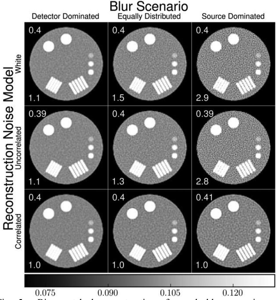
Fig. 5 shows bias matched reconstructions generated using each noise model in each blur scenario. Bias was matched at approximately 0.4 mm⁻¹ (indicated by the dotted lines in Fig 3) and an optimal (λ,β) pair was applied for each noise model. These reconstruction results illustrate the trends in Fig 3. When blur is predominately attributed to the source, using the correlated noise model results in a substantial reduction in noise. The noise reduction is less when the blur is equally distributed between source and detector, and is marginal when the blur is caused predominately by the detector.

Fig. 5.

Bias matched reconstructions for each blur scenario and reconstruction noise model. The bias of each reconstruction is shown in the top left (approximately 0.4 mm⁻¹), and the relative variance (the ratio of the noise variance in the reconstruction relative to the correlated noise variance) is shown in the bottom left of each image. Improved image quality (i.e., reduced noise) for the correlated noise model is evident in the equal blur and source blur dominated cases.

IV. DISCUSSION

In this work a generalized approach for reconstructing CT data with system blur and measurement correlations was introduced. The two step process involved a regularized deblurring step followed by a generalized penalized weighted least-squares reconstruction. Different noise models for the reconstruction were investigated including an approach that explicitly models the propagation of noise through the system and preprocessing. This explicit correlated model outperforms standard (uncorrelated) noise model choices. The benefits are greatest with more source blur, but are evident in a more typical scenario of balanced source and detector blur.

The proposed approach has potential application in tomographic systems that demand high spatial resolution and minimum noise/dose. Possible applications include flat-panel cone-beam CT systems, including dedicated dental, head, extremities, and mammography systems.

REFERENCES

- 1.Wang AS, Stayman JW, Otake Y, Kleinszig G, Vogt S, Gallia GL, Khanna aJ, Siewerdsen JH. Soft-tissue imaging with C-arm cone-beam CT using statistical reconstruction. Phys. Med. Biol. 2014 Feb;59(4):1005–1026. doi: 10.1088/0031-9155/59/4/1005. [DOI] [PMC free article] [PubMed] [Google Scholar]
- 2.Yu DF, Fessler Ja, Ficaro EP. Maximum-likelihood transmission image reconstruction for overlapping transmission beams. IEEE Trans. Med. Imaging. 2000 Nov;19(11):1094–1105. doi: 10.1109/42.896785. [DOI] [PubMed] [Google Scholar]
- 3.Feng B, Fessler Ja, King Ma. Incorporation of system resolution compensation (RC) in the ordered-subset transmission (OSTR) algorithm for transmission imaging in SPECT. IEEE Trans. Med. Imaging. 2006 Jul;25(7):941–949. doi: 10.1109/tmi.2006.876151. [DOI] [PubMed] [Google Scholar]
- 4.Hofmann C, Knaup M, Kachelriess M. Do We Need to Model the Ray Profile in Iterative Clinical CT Image Reconstruction? 2013:403. [Google Scholar]
- 5.Stayman JW, Zbijewski W, Tilley S, II, Siewerdsen J. Generalized Least-Squares CT Reconstruction with Detector Blur and Correlated Noise Models. :1–4. doi: 10.1117/12.2043067. [DOI] [PMC free article] [PubMed] [Google Scholar]