Abstract
This work investigates the statistics of the envelope of three-dimensional (3D) high-frequency ultrasound (HFU) data acquired from dissected human lymph nodes (LNs). Nine distributions were employed, and their parameters were estimated using the method of moments. The Kolmogorov Smirnov (KS) metric was used to quantitatively compare the fit of each candidate distribution to the experimental envelope distribution. The study indicates that the generalized gamma distribution best models the statistics of the envelope data of the three media encountered: LN parenchyma, fat and phosphate-buffered saline (PBS). Furthermore, the envelope statistics of the LN parenchyma satisfy the pre-Rayleigh condition. In terms of high fitting accuracy and computationally efficient parameter estimation, the gamma distribution is the best choice to model the envelope statistics of LN parenchyma, while, the Weibull distribution is the best choice to model the envelope statistics of fat and PBS. These results will contribute to the development of more-accurate and automatic 3D segmentation of LNs for ultrasonic detection of clinically significant LN metastases.
1. Introduction
Quantitative ultrasound (QUS) tissue parameters, such as the attenuation coefficient and spectral parameters, have proven their sensitivity to tissue microstructure.1) These approaches, commonly termed QUS or tissue-characterization, have been widely studied for their potential ability to classify normal vs abnormal tissue within kidney,2) breast,3) skin,4) prostate,5) and liver.6,7) QUS approaches using high-frequency (i.e., >15 MHz) ultrasound (HFU) provide an appropriate means of characterizing biological tissue with spatial resolutions on the order of 100 μm. HFU systems can successfully image shallow or low-attenuation tissues for biomedical applications. For example, HFU has already been successfully applied for small animal,8–10) ocular,11) intravascular,12,13) and dermatological imaging.14)
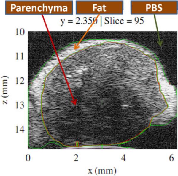
Previous work by our group has demonstrated that three dimensional (3D) high-frequency QUS can be used reliably to differentiate between fully-metastatic dissected human lymph nodes (LNs) and cancer-free LNs.15,16) In these prior studies, LNs were entirely imaged in 3D using HFU. Our QUS approach includes two key tasks: First, 3D segmentation, and second, 3D QUS-parameter estimation. The 3D segmentation process demarcates the LN parenchyma, fat and surrounding phosphate-buffered saline (PBS) as illustrated in Fig. 1. The result of segmentation then is used to correct QUS parameters estimated from LN parenchyma for attenuation and to limit QUS processing to LN parenchyma. Classification based on eight QUS parameters estimated from the LN parenchyma then is performed using linear-discriminant methods to detect metastatic parenchyma within the LN.15) This approach found that the combination of parameters reflecting the effective scatterer size and the homodyned-K statistical distribution of the envelope data provided an area under the ROC curve of 0.996 with specificity and sensitivity of 95% in a database of 112 LNs from 77 colorectal and gastric cancer patients. Despite this promising sensitivity, application of QUS for metastasis detection currently is limited by time-consuming visual inspection and manual correction required by the existing semi-automatic 3D segmentation method.15)
Fig. 1.
(Color online) HFU envelope data presenting a 2D section (in the x–z plane) selected from a volumetric data-set acquired from excised LN. Regions of LN parenchyma, fat and PBS as indicated by the labeled arrows were identified using a watershed-based, 3D segmentation method with manual revision of the boundaries by an expert.
Significant work has been performed to investigate the specific statistical properties of ultrasound echo-signal data within the clinically common frequency range (<15 MHz). Zimmer et al.17) used the lognormal distribution to model speckle in liver images. Shankar et al.3) proposed Nakagami and K distributions to model the backscattered echo signals from tissue, and the distribution parameters then were used to classify breast masses. A family of four distributions (gamma, Weibull, normal, and lognormal) was evaluated by Tao et al.18) for modeling the speckle in cardiac ultrasound images. The Tao study indicated that the gamma distribution provided the best fit to the data and had a low misclassification rate in distinguishing between blood and adjacent soft tissue. Nillesen et al.19) investigated the envelope statistics of blood and myocardium in echocardiographic images. The Nillensen study showed that the gamma distribution outperformed other distributions (K, Nakagami, inverse Gaussian, and Rayleigh) in describing the speckle statistics of blood and myocardium. To diagnose liver fibrosis, two and three component Rayleigh mixture models were proposed to model statistics of the ultrasonic envelope data acquired on this organ.20–22) Recently, Anquez et al.23) proposed the use of the gamma distribution to model the statistics in amniotic fluid and fetal tissues of antenatal 3D ultrasound images. Anquez then formulated a segmentation method by integrating the gamma statistical model of the intensity distribution using the maximum a posteriori (MAP) approach to maximize the probability p(P(Ω)|I) of the partition P(Ω) given the image I. Only a few studies have evaluated the statistics of HFU data. Raju et al.24) conducted a study on the statistics of the envelope of two-dimensional (2D) HFU backscatter signals from human skin. Raju's results indicated that the Weibull, K and generalized gamma distributions were capable of modeling the envelope statistics well. However, the shape parameters of the three distributions were unable to discriminate between data acquired in healthy skin and skin affected by dermatitis.4)
Our current work extends our previous investigation25) to identify probability density functions (PDFs) that best model the envelope of 3D HFU data acquired in LN parenchyma, fat and PBS. Once fully characterized, information regarding PDFs in different regions of the LN parenchyma and surrounding media can be applied to develop a more-robust LN segmentation method using the MAP approach.23,26) Furthermore, detailed characterization of parameters describing the PDF of non-cancerous vs metastatic LN parenchyma will contribute to more-accurate QUS-based characterization of LNs.
2. Methods
2.1 Ultrasound data acquisition
LN dissection, preparation for ultrasound data-acquisition and histological analysis have been described in detail.15,16,27) Only a brief summary is provided here. At the Kuakini Medical Center (KMC), excess perinodal fat was manually removed from LNs dissected from patients with histologically proven primary cancers and the nodes were placed in a room temperature PBS bath for ultrasonic scanning. Ultrasonic data acquisition used a focused, single-element transducer (Olympus PI30-2-R0.50IN) with an aperture of 6.1 mm, a focal length of 12.2 mm, a center frequency of 25.6 MHz, and a –6-dB bandwidth extending from 16.4 to 33.6 MHz. The theoretically predicted axial and lateral resolutions of the imaging system were 86 and 116 μm, respectively. Thus, the volume of 3D resolution cell can be estimated to be 9.08 μ 10–4 mm3. Radiofrequency (RF) echo signals were digitized at 400 MS/s using an 8-bit Acqiris DB-105 A/D board. Volumetric data were acquired from each LN by scanning adjacent planes with a uniform plane and A-line spacing of 25 μm in both lateral directions. Envelope data were derived from the digitized RF data by applying a Hilbert transform.
A database of 99 LNs dissected from colorectal-cancer patients was used to study the statistics of data at the focal distance (12.2 mm from the transducer). Eighteen nodes were entirely cancerous and 81 nodes were entirely devoid of cancer. Thirty-six LNs including 12 cancerous and 24 non-cancerous specimens were selected from the database to examine the statistics of LN data at, before and after the focal distance. These 36 LNs were selected because the semi-automatic segmentation technique provided accurate segmentation throughout the entire LN (not only for regions at the focal distance).
2.2 Probability density functions
The analytic signal associated to the signal backscattered from an ensemble of discrete scatterers in the absence of attenuation can be expressed at each instant as24) , where ai and φi, respectively, are the amplitude and phase of the backscattered signal from an individual scatterer i, and N is the number of scatterers, where the R denotes the envelope of the signals received by the transducer. The ai depends on the shape, size, and acoustical properties of each scatterer with respect to the surrounding medium. The φi depends on the position of each scatterer. The ai, φi, and N are unknown beforehand and can be modeled, in general, as random variables. Therefore, the resultant envelope R of the signal backscattered from an ensemble of discrete scatterers is also a random quantity that can be described using PDFs. Note that scattering in real tissue actually results from a continuous distribution of scattering sites throughout the tissue and not from discrete scatterers. However, this simplified model provides a convenient starting point for analysis. To determine which PDF best models the envelope of HFU data acquired from human LNs, we investigated the nine PDFs described in Table I. Each PDF is described briefly.
Table I.
Expression of the nine investigated PDFs. Here is the PDF of a standardized normal distribution, is the gamma function, ϕlogis(z) = ez(1 + ez)–2 is the PDF of a standardized logistic distribution.
| Family | Probability Density Function (r ≥ 0 unless specified) | Parameter interpretation |
|---|---|---|
| Rayleigh (RA) | σ > 0: scale | |
| Normal (NM) | μ: mean; σ > 0: standard deviation | |
| Lognormal (LM) | μ: location σ > 0: scale |
|
| Nakagami (NA) |
m ≥ 0.5: shape Ω > 0: scale |
|
| Weibull (WE) |
α > 0: scale β > 0: shape |
|
| Loglogistic (LL) |
μ: location σ > 0: scale |
|
| Gamma (GA) |
a > 0: shape b > 0: scale |
|
| Generalized extreme value (GE) | with |
k ≠ 0: shape μ: location σ > 0: scale |
| Generalized gamma (GG) |
a > 0, c > 0: shape b > 0: scale |
Rayleigh (RA) distribution
On the basis of the central-limit theorem, the envelope data, R, can be modeled using a RA distribution for either a large number of randomly distributed scatterers (the phase, φi, is uniformly distributed from 0 to 2π),28) or when the individual amplitudes ai are themselves RA distributed.24) The ratio of the mean of the RA distribution to its standard deviation, i.e., its SNR, has a constant value of 1.91.
Normal (NM) distribution
According to the central-limit theorem, the NM distribution approximately models the sum of a large number of independent, identically distributed (i.i.d.) random quantities. The NM distribution was used to describe the intensity distribution of ultrasound images of prostate tissue.29) It has recently been used to model the saturated 3D ultrasound data acquired from fetal tissue.23)
Lognormal (LM) distribution
The LM distribution is a common model for failures times. According to the central-limit theorem, the LM distribution can be used to model a random variable that arises from the product of a number of identically distributed independent positive random quantities.30) In the context of ultrasound, the LM distribution has been used to model the speckle in hepatic images.17)
Nakagami (NA) distribution
The NA distribution was first proposed by Nakagami to describe the statistics of returned radar echoes.31) The parameter m is constrained such that m ≥ 0.5.31) The study by Yacoub32) indicated that the magnitude of the incoherent sum of powers (as opposed to the instantaneous amplitude summation) of several RA signals can be modeled by the NA distribution. In the context of ultrasound, Shankar28) proved that pre-Rayleigh (SNR < 1.91), Rayleigh (SNR = 1.91) and post-Rayleigh (SNR > 1.91) conditions could be modeled by the Nakagami distribution. Moreover, Shankar showed that the envelope of backscattered signals obtained from human breast was described well by this distribution and that its parameters could be used to classify breast masses.33) The NA distribution includes the RA distribution for the special case when m = 1, and approximates the Rician distribution when m > 1.
Weibull (WE) distribution
The WE distribution has been used to model radar clutter signals.34) The statistics of the envelope of high-frequency ultrasonic backscatter from human skin have been approximately described by this distribution.24) Because the SNR monotonically increases with the shape parameter β, the WE distribution can be used to model pre-Rayleigh (0 < β < 2), Rayleigh (β = 2) and post-Rayleigh (β > 2) conditions. Note that, the WE distribution includes the exponential (β = 1) and RA (β = 2) distributions. Furthermore, if R has a WE distribution with parameters α and β, then U = ln(R) has an extreme value distribution with μ and δ parameters, where μ = ln(α), and δ = β–1.
Loglogistic (LL) distribution
The LL distribution is often used in survival analysis to model events that experience an initial rate increase, followed by a rate decrease. The LL distribution is considered here because it has a shape that is similar to the shape of the LM distribution; however the LL distribution has heavier tails, i.e., the tails of the histogram at high and low values are heavier.30)
Gamma (GA) distribution
The sums of exponentially distributed random variables can be well modeled by the GA distribution. If parameter a is large, the GA distribution closely approximates a NM distribution when modeling only positive real numbers. The GA distribution includes the exponential distribution when b = 1, and also includes the chi-squared distribution with n degrees of freedom when a = 1/2 and b = n/2. Moreover, if R has a NA distribution with parameters m and Ω, then R2 has a GA distribution with a shape parameter m and a scale parameter Ω/m. Because the shape parameter a takes values in the range 0 < a < ∞, using the GA distribution eliminates the constraint (m ≥ 0.5) that is imposed when using the NA distribution. In the context of ultrasound, the GA distribution was shown to well describe the envelope of backscatter signals obtained from amniotic fluid and fetal tissues.23)
Generalized extreme value (GE) distribution
The GE distribution was developed within extreme value theory to combine the Gumbel (k = 0), Frechet (k > 0), and WE (k < 0) families; it also corresponds to the type I, type II, and type III extreme value distributions.35) The GE distribution is often used as an approximation to model the maxima of long finite sequences of random variables. We consider this distribution because the envelope of ultrasound echo-signal data presents local maxima.
Generalized gamma (GG) distribution
By adding a third parameter to the GA distribution, Stacy36) introduced the GG distribution. Shankar37) proposed the use of the GG distribution to model the envelope of ultrasonic signals backscattered from breast tissue. Subsequently, the GG dis tribution was demonstrated to describe the envelope of 2D HFU signals backscattered from human skin.24) An interesting property of the GG distribution is its ability to model amplitude as well as intensity fluctuations [if R is GG distributed, R2 and kR (where k is a constant) are also GG distributed]. This distribution also includes the following distributions as special cases: RA (c = 2, a = 1), exponential (c = 1, a = 1), NA (c = 2), WE (a = 1), GA (c = 1), and LM (a → ∞).
2.3 Parameter estimation
The parameters of each distribution that best corresponded to the envelope data were estimated according to the following relations using the method of moments.38) This method derives parameters from the moment of the data and provides computational efficiency. For convenience, the M envelope samples in the region of interest were assumed to be i.i.d., and denotes the sample mean the envelope R.
RA distribution
The scale parameter δ of the RA distribution can be effectively estimated as .
NM distribution
The mean and standard deviation parameters of the NM distribution can be estimated using
LM distribution
The NM and LM distributions are closely related. If R is distributed lognormally with parameters μ and δ, then U = ln(R) is distributed normally with mean μ and standard deviation δ. Consequently, the location and scale parameters of the LM distribution can be efficiently estimated as , and .
NA distribution
The method of moments can be used to obtain the two parameters of the NA distribution as follows
| (1) |
| (2) |
The estimation of the m parameter using (2) is computationally efficient. However, the constraint (m ≥ 0.5) was violated by our data. Therefore, we used the m estimator devised by Greenwood and Durand39) because it best approximates to the maximum-likelihood estimator as indicated by Zhang.40)
| (3) |
where , with a sample estimate of the kth moment , and .
WE distribution There are no closed-form expressions for estimating the β parameter of the WE distribution. Using the method of moments, the parameter β can be estimated by solving the following implicit equation:
| (4) |
A unique solution of exists because the left hand side (LHS) of (4) is a monotonic function of . A look-up table with precomputed values of the LHS as a function of finely spaced (estimation accuracy of 0.0001 for 0:1 ≤ ≤ 5:0) was used to obtain . After obtaining , was estimated from the equation, .
LL distribution
The LL distribution is closely related to the logistic distribution. If R is distributed loglogistically with parameters μ and δ, then U = ln(R) is distributed logistically with parameters μ and δ. Consequently, the parameters of the LL distribution are estimated using the method of moments as, , and .
GA distribution
Using the of method, the parameters of the GA distribution can be efficiently estimated as , and .
GE distribution
There is no closed-form solution for the parameter estimation of the GE distribution. Therefore, its three parameters were estimated using a maximum likelihood algorithm.35)
GG distribution
The three parameters of the GG distribution can be estimated using the moment of the logarithm of the data:41)
| (5) |
| (6) |
| (7) |
where U = ln(R), and is the polygamma function. The LHS of (5) is a monotonic function of â. The solution of (5) was found by using a look-up table with precomputed values of the LHS as a function of finely spaced â (estimation accuracy of 0.001 for 0:1 ≤ â 50:0). Once â was obtained, the parameters ĉ and b̂ were estimated using (6) and (7), respectively.
2.4 Extraction of 3D regions-of-interest (ROIs)
The extraction of the ROIs plays a crucial role in statistical analysis. The size of each ROI must be large enough to contain a sufficient number of resolution cells for the hypothesis that every envelope voxel within the ROI is independent and identically distributed to be valid. On the other hand, the ROI must be small enough to provide acceptable spatial resolution, and to avoid getting signals affected by very different attenuation and diffraction effects. To mitigate potential bias related to LN size, a maximum of ten non-overlapping, randomly-located ROIs at a fixed depth (distance from the transducer) were selected for LN parenchyma, fat and PBS. Any ROIs that were not fully included in depths between 10.85 to 13.55 mm were not processed because they were considered to be too distant from the focal zone of the transducer.
2.4.1 LN parenchyma and PBS
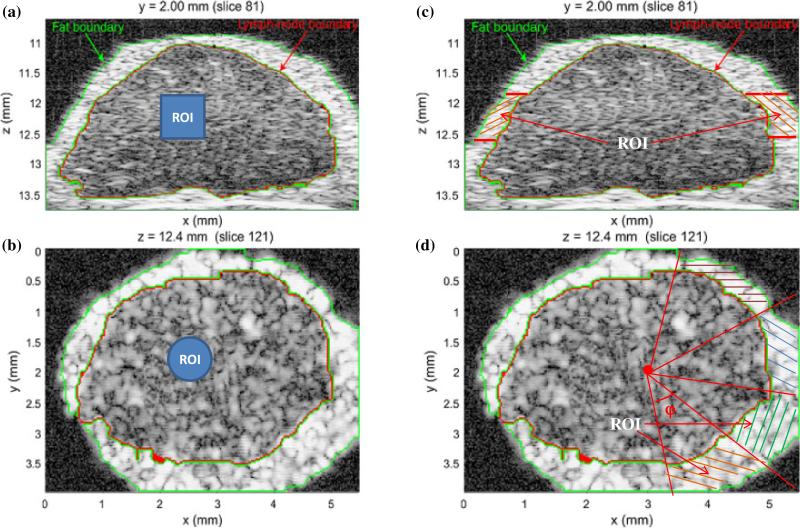
For statistical analysis of the LN parenchyma and PBS, non-overlapping, randomly-located cylindrical ROIs with a 0.7 mm length and diameter were extracted from the envelope data. The number of independent resolution cells for each 3D ROI was [π(700/ 2)2 × 700]/[π(116/2)2 × 86] ~ 296, because the predicted axial and lateral resolutions of the imaging system were 86 and 116 μm, respectively. The centers of the ROIs were located at depths of 11.2 mm, 12.2 mm (focal distance), 13.2 mm. Figures 2(a) and 2(b) present the z–x and y–x cross-sectional planes, respectively, to illustrate the ROI dimensions in the LN parenchyma. The number of ROIs for the LN parenchyma and PBS at the focal distance of the 99 LNs were 967 and 468, respectively, since some small LNs provided fewer than 10 ROIs.
Fig. 2.
(Color online) Illustration of the dimensions and positioning of a cylindrical ROI (solid blue region) in the LN parenchyma in the x–z plane (a) and the x–y plane (b). Similar positioning and ROI size was used to select ROIs in the PBS. The division of the fat layer into angular sections is illustrated by the cross-hatched regions in the x–z plane (c) and the x–y plane (d).
2.4.2 Fat
Because the layer of fat surrounding the LN parenchyma is very thin and varied in extent, use of cylindrical ROIs within the fat region of each LN is not practical. Consequently, ROIs were extracted from the fat layer as illustrated in Figs. 2(c) and 2(d). For each LN, the ROIs in the fat layer were placed so that the number, N, of voxels within each ROI was equal to the number within the ROIs of the LN parenchyma or PBS. First, a 3D fat-mask section with a depth range of 0.7 mm and central depth of 11.2, 12.2, or 13.2 mm, respectively, was prepared using the manually segmented fat label [Fig. 2(c)]. Second, within the x–y plane, triangular sections were delimited so that the apex was at the center of the LN. The angle φ of each 3D triangular section was adjusted so that the number of fat-mask voxels contained in a 3D triangular section (with a slice-thickness of 0.7 mm) equaled to N. Finally, the voxels within the fat (as delimited by the section thickness and the triangular sections) were treated as an independent ROI for statistical analysis. The number of fat ROIs at the focal distance of the 99 LNs is 956.
2.5 Goodness-of-fit evaluation
To evaluate quantitatively the goodness of fit of each candidate distribution to the experimental envelope distribution, the Kolmogorov Smirnov (KS) metric42) was used. The KS metric is the maximum absolute difference between the theoretical cumulative distribution function (CDF) [F(x)] and the experimental envelope CDF [G(x)]; it is given by MKS(F, G) = max |F(x) – G(x)|. Smaller values of the KS metric indicate a better fit of the candiadate distribution to the experimental distribution.
3. Results
3.1 Models describing the statistics of envelope data of LN parenchyma, fat and PBS
To facilitate comparing distributions, the vertical axes of all the box plots representing the KS metrics are presented on a log scale. For each box, the central mark is the median, the edges of the box are the 25th and 75th percentiles, the whiskers extend to the most extreme data points that are not considered outliers, and outliers are plotted individually. Points are drawn as outliers if they are larger than q3 + 1.5(q3 – q1) or smaller than q1 – 1.5(q3 – q1), where q1 and q3 are the 25th and 75th percentiles, respectively.
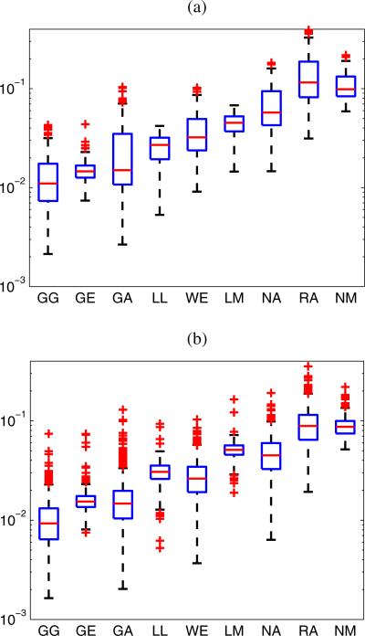
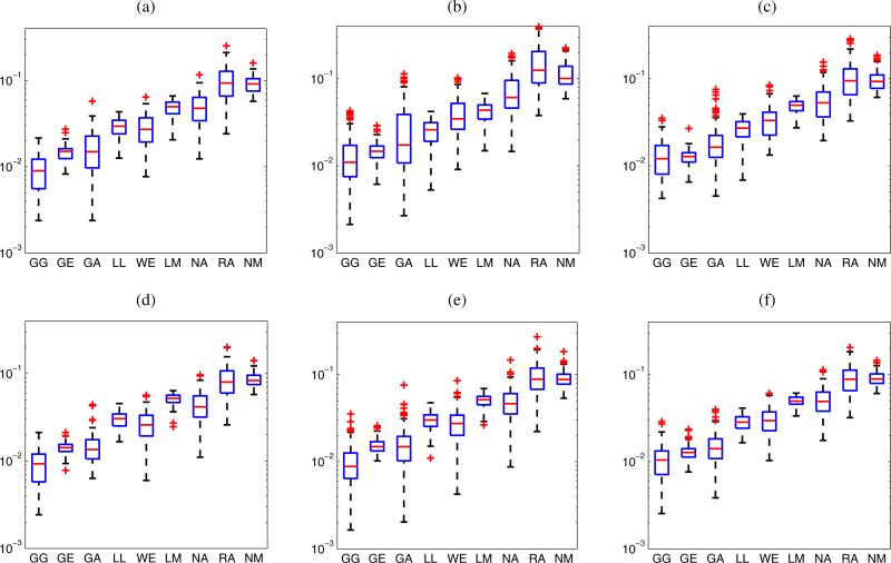
The GG distribution best modeled the statistics for 66.4, 65.2, and 61.1% of the ROIs of LN parenchyma, fat and PBS centered at the focal distance, respectively. The GG distribution also provided the lowest average values of the KS metric for the 967 LN parenchyma, 956 fat and 468 PBS ROIs. Figure 3 shows box plots of the KS metrics for the data from LN parenchyma ROIs of the 18 cancerous LNs and the 81 non-cancerous LNs. The plots illustrate how the GG distribution best fits the experimental envelope distribution of both cancerous and non-cancerous LNs. The GG distribution provides the lowest median values of the KS metrics for cancerous LNs (0.011) and non-cancerous LNs (0.009). Therefore, the GG distribution outperforms all the 8 remaining distributions (GE, GA, LL, WE, LM, NA, RA, NM) in fitting the envelope distributions from the three different media.
Fig. 3.
(Color online) KS metrics for all the LN parenchyma ROIs centered at the focal distance. Eighteen cancerous LNs (a), and 81 non-cancerous LNs (b).
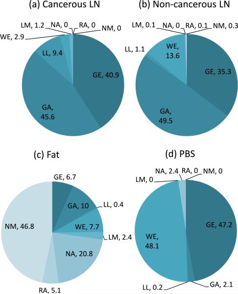
To investigate which distributions other than the GG distribution best describe the statistics of HFU envelope data acquired in cancerous and non-cancerous LNs at the focal distance, the percentage of ROIs best modeled by the remaining 8 distributions (excluding the GG distribution) was evaluated based on the KS metric. Results are summarized in Fig. 4. As shown in Fig. 4(a), the GA and GE distributions best model the statistics for 45.6 and 40.9%, respectively, of the cancerous LN parenchyma ROIs. Thus they have approximately the same fitting performance and outperform all the remaining six distributions. Among the 81 non-cancerous LNs, the GA distribution best models the statistics for 49.5% of ROIs, followed by the GE distribution with 35.3%, as illustrated in Fig. 4(b). Consequently, the GA distribution fits most of the experimental envelope distribution of non-cancerous LNs better than the GE distribution does, as also indicated in Fig. 3(b).
Fig. 4.
(Color online) Percentages of ROIs from each medium that were best modeled by each of the eight distributions (excluding GG) as assessed using the KS metric. All ROIs were centered at the focal distance.
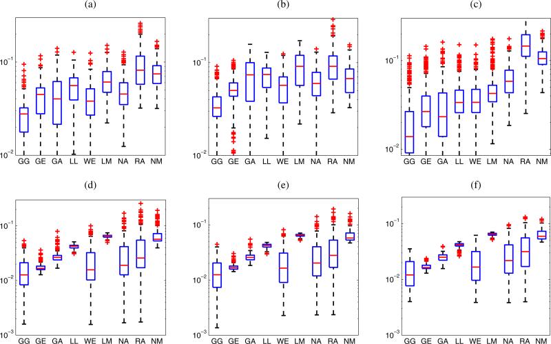
Figure 5 presents the KS metrics for LN parenchyma ROIs centered at depths of 11.2, 12.2, and 13.2 mm, respectively, for the 12 cancerous LNs and 24 non-cancerous LNs. The GG distribution best describes the statistics of ROIs at each depth, followed by the GA and GE distributions. Among the 12 cancerous LNs, the GE distribution fits the experimental envelope distribution slightly better than the GA distribution as shown in Figs. 5(a)–5(c). Furthermore, the distribution of the KS metrics of the GA distribution for cancerous LNs is broader than that for the non-cancerous LNs. However, the GA distribution is likely to describe the statistics of ROIs of non-cancerous LNs marginally better than the GE distribution as indicated in Figs. 5(d)–5(f ).
Fig. 5.
(Color online) KS metrics for LN parenchyma ROIs of 12 cancerous LNs (a–c) and 24 non-cancerous LNs (d–f). The ROIs are centered at different depths: (a, d) 11.2 mm; (b, e) 12.2 mm; (c, f) 13.2 mm.
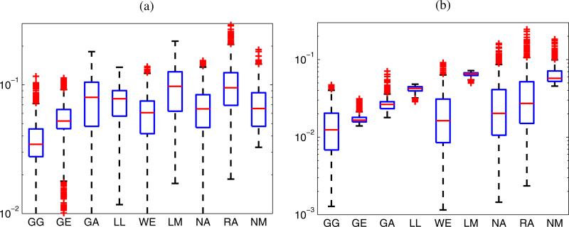
Regarding the statistics of the envelope of the HFU data acquired in the fat layer at the focal distance, Fig. 6(a) presents a box plot of the KS metrics for fat ROIs centered at the focal distance of the 99 LNs. The GG distribution again shows the best fit by providing lowest KS metrics. The median of KS metrics of the GG distribution for fat is 0.034 which is much higher than that for the LN parenchyma. The data summarized in Fig. 4(c) show that the NM distribution outperforms the other 7 distributions (excluding the GG distribution) by best describing the statistics of 46.8% of the fat ROIs. Nevertheless, the distribution of the KS metrics of the NM, WE, NA distributions are relatively similar as presented in Fig. 6(a). The WE distribution is superior to the NM and NA distributions because it has the lowest KS-metric median. The KS metrics for fat ROIs centered at different depths, 11.2, 12.2, and 13.2 mm are shown in Fig. 7. While the GG distribution always outperforms the other distributions, the NM distribution is fairly good at the focal distance, that is when the 75th percentile of the KS metrics of the GA distribution is the worst of the three 75th GA percentiles. Away from the focal distance, apart from the GG distribution, the WE, GA, and GE distributions provide reasonable alternatives as shown in Figs. 7(a) and 7(c).
Fig. 6.
(Color online) KS metrics for Fat (a) and PBS (b) ROIs centered at the focal distance of the 99 LNs.
Fig. 7.
(Color online) KS metrics for fat ROIs (a–c) and PBS ROIs (d–f ) of the 36 LNs. The ROIs are centered at different depths: (a, d) 11.2 mm; (b, e) 12.2 mm; (c, f ) 13.2 mm.
The statistics of the envelope data obtained from the PBS at the focal distance are best modeled by the WE and GE distributions (when The GG is excluded) as 48.1 and 47.2% of the PBS ROIs, respectively, as shown in Fig. 4(d). The NA and GA distributions best describe the statistics of 2.4 and 2.1% of the ROIs. The same result is illustrated in Fig. 6(b), whereas the GG distribution obtains the best fit with the lowest median value of the KS metric (0.012), followed by the WE and GE distributions. To examine the envelope statistics for HFU data in PBS at different depths, the KS metrics for the PBS ROIs centered at the depths of 11.2, 12.2, and 13.2 mm, respectively, are shown Figs. 7(d), 7(e), and 7(f ). In the descending order of fitting accuracy, the GG, WE, GE, NA, GA, and RA distributions best model the statistics of the PBS data. This is true at all the depths considered. Ideally, the PBS region contains no scatterers so statistics are anticipated to be those of the noise. Table II summarizes the distributions that best model the three media encountered in LN data ranked according to their relative accuracy as assessed using the KS metric.
Table II.
Distributions best describing the envelope of HFU data as assessed using the KS metric. From left to right the distributions are listed in the order of descending accuracy.
| Medium | Best-fit distributions |
|---|---|
| Parenchyma | GG > GA> GE > WE |
| Fat | GG > WE > GA/NA > GE |
| PBS | GG > WE > GE > NA/GA/RA |
Figure 8 shows the experimental PDFs for three representative ROIs corresponding to each of the three media, as well as their best estimated PDFs and the associated KS metrics. The GG and GA distributions fit the experimental envelope of the LN parenchyma very well in both tails as illustrated in Fig. 8(a). Although the GG and WE distributions best model the statistics of fat among the all other distributions, their KS metrics are higher than those of the LN parenchyma and PBS. This can be explained by the complicated experimental envelope distribution of the fat as shown in Fig. 8(b), which results from the saturation occurring during digitization. In the fat, the correlation coefficients between the percentage of saturated voxels in the HFU data and the KS metrics of the GG, WE and GA distributions are 0.70, 0.79, and 0.95, respectively. In particular, the KS metric values increase significantly as the percentage of saturated voxels in the HFU data increases.
Fig. 8.
(Color online) Experimental envelope PDF from representative LN parenchyma ROI (a), fat ROI (b), and PBS ROI (c). Fits and associated KS metrics are shown for the best-fitting distributions.
3.2 Parameter examination
The SNR of the envelope of all LN parenchyma ROIs are less than 1.91 (SNR = 1.50 ± 0.16). This result indicates that the PDF of the LN parenchyma envelope satisfies the pre-Rayleigh condition.
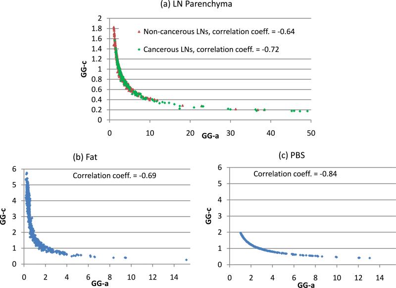
Because the GG distribution best models the envelope data of the LN parenchyma, fat and PBS, an examination of its parameters is worthwhile. As presented in Sect. 2.2, the GG distribution has a single scale parameter (GG-b) and two shape parameters (GG-a, GG-c). GG-b was not included in the study because it strongly depend on attenuation and examined depth. Depending on the values of the two shape parameters, the GG distribution may include RA (c = 2, a = 1), exponential (c = 1, a = 1), NA (c = 2), WE (a = 1), GA (c = 1), and LM (a → ∞) distributions. Figure 9 shows the relationship between the two shape parameters of the GG distribution for the three media. ROIs at the focal zone of 18 cancerous LNs and 81 non-cancerous LNs were considered. Figure 9 indicates significant correlations between the two shape parameters for the three media. As GG-a increases, GG-c decreases considerably. As shown in Fig. 9(a), GG-c never reaches the value of 2; this means that among the family of the GG distribution, the RA and NA distributions do not well model the envelope data of LN parenchyma, as reported in Sect. 3.1. Figure 9(a) also shows a large overlap between the two shape parameters of cancerous LN ROIs and non-cancerous LN ROIs except when the GG-a parameter is greater than approximately 10. Therefore, using the two shape parameters to characterize between cancerous and non-cancerous LN ROIs can be expected to be ineffective. Nevertheless, Fig. 9 illustrates that the ranges of values of the two shape parameters are different from one media to another but those ranges do overlap considerably.
Fig. 9.
(Color online) The relation between two shape parameters (GG-a, GG-c) of the GG distribution for different media. The correlation coefficients between GG-a and GG-c are also indicated.
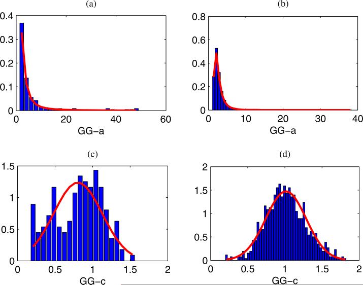
Figures 10(a) and 10(b) present the histograms of the GG-a values for 166 cancerous LN ROIs and 793 non-cancerous LN ROIs, respectively, centered at the focus. The GE distribution can model their distributions by providing lowest KS statistic values. Similarly, Figs. 10(c) and 10(d) show the distributions of the GG-c values for 166 cancerous LN ROIs and 793 non-cancerous LN ROIs, respectively. The NM distribution can serve as models for their distributions. The Lilliefors43) test does not reject the null hypothesis at the 5% significant level. (The estimated GG-c parameters comes from a NM distribution.) The p-values returning from the Lilliefors tests for cancerous LN ROIs and non-cancerous LN ROIs are 0.047 and 0.258, respectively. Table III presents the estimated parameters of the GE and NM distributions used to model the GG-a and GG-c values as well as their corresponding KS-statistic values. As shown in Table III, the mean of the distribution of the GG-c values for the envelope data from non-cancerous LN ROIs is 1.01 (approximately 1). This is in agreement with the KS metrics results presented in Sect. 3.1 that show that the GA distribution (GG-c = 1) very often can model the envelope data of LN parenchyma well.
Fig. 10.
(Color online) The distribution of the two shape parameters of the GG distribution and overlaid fits. (a, b) Distributions of the GG-a parameter of cancerous LNs and non-cancerous LNs. (c, d) Distributions of the GG-c parameter of cancerous LNs and non-cancerous LNs. The overlaid fits of the distributions of the GG-a and GG-c parameters are the Generalized Extreme Value and Normal distributions, respectively.
Table III.
Estimated parameters of the GE and NM distributions that best model the distribution of the GG-a and GG-c parameters and their respective KS statistic.
| GE modeling of the distribution of the GG-a par. |
NM modeling of the distribution of the GG-c par. |
|||||||
|---|---|---|---|---|---|---|---|---|
| ROIs type | Shape | Scale | Location | KS stat. | ROIs type | Mean | Std. Dev. | KS stat. |
| Cancerous | 0.83 | 1.39 | 2.64 | 0.06 | Cancerous | 0.80 | 0.32 | 0.071 |
| Non-cancerous | 0.29 | 0.74 | 2.11 | 0.023 | Non-cancerous | 1.01 | 0.27 | 0.025 |
Correspondingly, the GE distribution could be used to model the distributions of the GG-a parameters for the PBS ROIs at the focus. However, the NM distribution does not model the GG-c parameters for the PBS ROIs well at the focus. Moreover, the GE and NM distributions do not model the distributions of the GG-a and GG-c values, respectively, of fat ROIs at the focus well: KS-metric values are high and the Lilliefors test rejects the null hypothesis for the GG-c values from the NM distribution.
4. Discussion and conclusions
This work evaluates the statistics of 3D HFU envelope-signal data obtained from dissected human LNs. The results of the study indicate that the GG distribution best models the three different media (LN parenchyma, fat and PBS) interrogated during volumetric scanning because it produces the lowest values of the KS metric. The two shape parameters, GG-a and GG-c, of the GG distribution improve the fit of the heavier tails of the experimental PDFs. The GG distribution includes many distributions commonly used to characterize the speckle: gamma, Weibull, Nakagami, Rayleigh, exponential, and lognormal. Therefore, it has all the advantages of these distributions. Although some differences exist between the two sets of shape parameters for the GG distribution, they do show significant overlap between cancerous and non-cancerous LN ROIs. Thus, use of these shape parameters for characterization of LN types could be investigated further, but at present, they seem to be of limited interest. The GG distribution has three parameters, and the high correlation between its two shape parameters (GG-a, GG-c) means that the envelope data could be effectively modeled by a 2-parameter distribution. However, the parameter estimation of the GG distribution is computationally expensive. Hence the use of the GG distribution in segmentation is not attractive. Alternatively, the two-parameter GA distribution also well described the envelope statistics for LN parenchyma data (as shown in Figs. 3–5). Its parameters can be estimated efficiently. Therefore, the GA distribution could provide a good option for modeling the signal from LN parenchyma.
Closer examination of the physical interpretation of the distribution statistics can help understand why the Rayleigh distribution does not describe the data adequately. In ultra-sound imaging, echo-signal envelope data statistics are described well by the Rayleigh distribution only when every resolution cell contains a large number of identical scatterers that are randomly and uniformly distributed. We applied our previously reported method15) to estimate the two parameters (the effective number of scatterers, μ, per resolution cell and the ratio, k, of the coherent to diffuse signal) of the homodyned-K distribution for the 967 LN parenchyma ROIs centered at the focal distance (without compensation for attenuation). The average value of μ was 1.04 for cancerous LN, and 1.81 for non-cancerous LN. These values for the effective number of scatterers are too small (much smaller than 1044,45)) to provide typical Rayleigh behavior and is consistent with the observed pre-Rayleigh behavior (SNR = 1.50 ± 0.16). Furthermore, the average value of k was determined to be on the order of 0.57. This implies the existence of a non-negligible coherent signal, which is not a typical feature for data satisfying the Rayleigh conditions. The small number of effective scatterers per resolution cell may be partly driven by small resolution cell size (9.08 × 10⁻⁴ mm3) obtained with the HFU imaging system. Although the tissue structures associated with the coherent signal have not been specifically identified, LNs are known to have a complex structure, and elements of this structure may contribute to producing speckle statistics that do not conform to the Rayleigh distribution. LN can be considered to be “kidney shaped” with an outer cortical layer surrounding an inner core of parenchyma and a central fatty hilum region. The cortex consists of numerous afferent lymph ductules and intertwined capillaries. These eventually converge toward small efferent ducts and blood vessels. Therefore, acoustic response from structures with very different scattering properties can be anticipated. Moreover, echoes from spatially extended structures such as the efferent vessels in the LNs may be strongly correlated (spatially coherent scattering). Clearly, to the extent that the different structures in the LN are scatterers, their sizes tend to change and increase toward the hilum. Furthermore, their orientations may depend on location within the node. Hence the scattering properties within a ROI may vary over the ROI and be dependent on the size and location of the ROI. This diversity of scatterers and their properties within the ROI may result in multiple distributions in the envelope statistics being expressed.
To describe the statistics of the envelope of the HFU in fat, the WE distribution appeared to be the most appropriate. Although the GG and WE distributions model the envelope data from fat better than the remaining distributions, their fitting accuracy is not very good due to the complicated experimental PDF caused by saturation of the HFU echo signals from the fat layers. In effect, the input-voltage range of the digitizer was optimized for acquisition of data from the LN parenchyma (regions in which estimated QUS parameters are of clinical interest). Consequently, to segment the media based on parametric modeling of the envelope, a preprocessing step (such as low-pass filtering) should be applied to the HFU data to re-estimate the saturated signals prior to calculating the envelope data. Note that the GE distribution modeled the statistics of the envelope data well for fat as well as LN parenchyma. Nevertheless, the GE distribution is not a good candidate for incorporation in segmentation techniques because of the complicated expression for the PDF and the time-consuming estimation of parameters required to fit this expression. For envelope data from regions within the PBS, the WE provided best accuracy. The GA distribution performed next best for the characterization of statistics for data from PBS. The NA and RA distributions also demonstrate an ability to model the statistics of the PBS as shown in Fig. 8(c). In the PBS, the KS metric is independent of the depth because the recorded signal in this medium were due to the noise from the acquisition system and not to backscattered echoes from scatterers.
In conclusion, based on these findings, the statistical distributions that appear to be the most promising to describe the envelope data adequately with minimal calculation time are the GA for LN parenchyma and the WE for fat and PBS. This provides a solid starting point for future work to incorporate the statistics of the three media into robust algorithms for segmentation of HFU data from human LNs.
Acknowledgements
This research was supported in part by the NIH grant CA100183 awarded to Riverside Research, Ernest Feleppa, Principal Investigator. The authors also acknowledge “Fellowship for Research in Japan” funding (S-13162) received from the Japan Society for the Promotion of Science (JSPS) awarded to Alain Coron in 2013.
References
- 1.Lizzi FL, Ostromogilsky M, Feleppa EJ, Rorke MC, Yaremko MM. IEEE Trans. Ultrason. Ferroelectr. Freq. Control. 1987;34:319. doi: 10.1109/t-uffc.1987.26950. [DOI] [PubMed] [Google Scholar]
- 2.Lizzi FL, Greenebaum M, Feleppa EJ, Elbaum M, Coleman DJ. J. Acoust. Soc. Am. 1983;73:1366. doi: 10.1121/1.389241. [DOI] [PubMed] [Google Scholar]
- 3.Shankar PM, Dumane VA, George T, Piccoli CW, Reid JM, Forsberg F, Goldberg BB. Phys. Med. Biol. 2003;48:2229. doi: 10.1088/0031-9155/48/14/313. [DOI] [PubMed] [Google Scholar]
- 4.Raju BI, Swindells KJ, Gonzalez S, Srinivasan MA. Ultrasound Med. Biol. 2003;29:825. doi: 10.1016/s0301-5629(03)00009-7. [DOI] [PubMed] [Google Scholar]
- 5.Feleppa EJ, Porter CR, Ketterling JA, Lee P, Dasgupta S, Urban S, Kalisz A. Ultrason. Imaging. 2004;26:163. doi: 10.1177/016173460402600303. [DOI] [PMC free article] [PubMed] [Google Scholar]
- 6.Yamaguchi T, Hachiya H. J. Med. Ultrason. 2010;37:155. doi: 10.1007/s10396-010-0270-y. [DOI] [PubMed] [Google Scholar]
- 7.Shiina T, Maki T, Yamakawa M, Mitake T, Kudo M, Fujimoto K. Jpn. J. Appl. Phys. 2012;51:07GF11. [Google Scholar]
- 8.Turnbull DH. Methods Mol. Biol. 2000;135:235. doi: 10.1385/1-59259-685-1:235. [DOI] [PubMed] [Google Scholar]
- 9.Aristizábal O, Christopher DA, Foster FS, Turnbull DH. Ultrasound Med. Biol. 1998;24:1407. doi: 10.1016/s0301-5629(98)00132-x. [DOI] [PubMed] [Google Scholar]
- 10.Mamou J, Aristizabal O, Silverman RH, Ketterling JA, Turnbull DH. Ultrasound Med. Biol. 2009;35:1198. doi: 10.1016/j.ultrasmedbio.2008.12.017. [DOI] [PMC free article] [PubMed] [Google Scholar]
- 11.Silverman RH, Ketterling JA, Mamou J, Coleman DJ. Arch. Ophthalmol. 2008;126:94. doi: 10.1001/archopht.126.1.94. [DOI] [PMC free article] [PubMed] [Google Scholar]
- 12.Saijo Y, Tanaka A, Owada N, Akino Y, Nitta S. Ultrasonics. 2004;42:753. doi: 10.1016/j.ultras.2003.11.022. [DOI] [PubMed] [Google Scholar]
- 13.Oshiro O, Kamada K, Chihara K, Secomski W, Nowicki A. Jpn. J. Appl. Phys. 2000;39:3216. [Google Scholar]
- 14.Huang YP, Zheng YP, Leung SF, Choi AP. Ultrasound Med. Biol. 2007;33:1191. doi: 10.1016/j.ultrasmedbio.2007.02.009. [DOI] [PubMed] [Google Scholar]
- 15.Mamou J, Coron A, Oelze ML, Saegusa-Beecroft E, Hata M, Lee P, Machi J, Yanagihara E, Laugier P, Feleppa EJ. Ultrasound Med. Biol. 2011;37:345. doi: 10.1016/j.ultrasmedbio.2010.11.020. [DOI] [PMC free article] [PubMed] [Google Scholar]
- 16.Coron A, Mamou J, Saegusa-Beecroft E, Oelze ML, Yamaguchi T, Hata M, Machi J, Yanagihara E, Laugier P, Feleppa EJ. Proc. Int. Symp. Biomedical Imaging. 2012:1064. doi: 10.1109/EMBC.2012.6346130. [DOI] [PubMed] [Google Scholar]
- 17.Zimmer Y, Tepper R, Akselrod S. Proc. World Congr. Medical Physics and Biomedical Engineering. 2000:23. [Google Scholar]
- 18.Tao Z, Tagare HD, Beaty JD. IEEE Trans. Biomed. Eng. 2006;25:1483. doi: 10.1109/TMI.2006.881376. [DOI] [PubMed] [Google Scholar]
- 19.Nillesen MM, Lopata RGP, Gerrits IH, Kapusta L, Thijssen JM, Korte CLD. Ultrasound Med. Biol. 2008;34:674. doi: 10.1016/j.ultrasmedbio.2007.10.008. [DOI] [PubMed] [Google Scholar]
- 20.Igarashi Y, Yamaguchi T, Hachiya H. Jpn. J. Appl. Phys. 2011;50:07HF17. [Google Scholar]
- 21.Koriyama A, Yasuhara W, Hachiya H. Jpn. J. Appl. Phys. 2012;51:07GF09. [Google Scholar]
- 22.Higuchi T, Hirata S, Yamaguchi T, Hachiya H. Jpn. J. Appl. Phys. 2013;52:07HF19. [Google Scholar]
- 23.Anquez J, Angelini ED, Grange G, Bloch I. IEEE Trans. Biomed. Eng. 2013;60:1388. doi: 10.1109/TBME.2012.2237400. [DOI] [PubMed] [Google Scholar]
- 24.Raju BI, Srinivasan MA. IEEE Trans. Ultrason. Ferroelectr. Freq. Control. 2002;49:871. doi: 10.1109/tuffc.2002.1020157. [DOI] [PubMed] [Google Scholar]
- 25.Bui TM, Coron A, Mamou J, Saegusa-Beecroft E, Yamaguchi T, Yanagihara E, Machi J, Bridal SL, Feleppa EJ. Proc. Symp. Ultrasonic Electronics. 2013 [Google Scholar]
- 26.Slabaugh G, Unal G, Weils M, Fang T, Rao B. Ultrasound Med. Biol. 2009;35:781. doi: 10.1016/j.ultrasmedbio.2008.10.014. [DOI] [PubMed] [Google Scholar]
- 27.Mamou J, Coron A, Hata M, Machi J, Yanagihara E, Laugier P, Feleppa EJ. Jpn. J. Appl. Phys. 2009;48:07GK08. [Google Scholar]
- 28.Shankar PM. IEEE Trans. Ultrason. Ferroelectr. Freq. Control. 2000;47:727. doi: 10.1109/58.842062. [DOI] [PubMed] [Google Scholar]
- 29.Shao F, Ling K, Ng W. Int. J. Image Graphics. 2004;04:385. [Google Scholar]
- 30.Meeker WQ, Escobar LA. Statistical Method for Reliability Data. Wiley; New York: 1998. [Google Scholar]
- 31.Nakagami M. In: Statistical Methods of Radio Propagation. Hoffman WC, editor. Pergamon; New York: 1960. p. 3. [Google Scholar]
- 32.Yacoub MD. IEEE Antennas Propag. Mag. 2000;42:150. [Google Scholar]
- 33.Shankar PM, Dumane VA, Reid JM, Genis V, Forsberg F, Piccoli CW, Goldberg BB. IEEE Trans. Ultrason. Ferroelectr. Freq. Control. 2001;48:569. doi: 10.1109/58.911740. [DOI] [PubMed] [Google Scholar]
- 34.Fernandes D, Sekine M. IEICE Trans. Commun. 1993;E76-B:1231. [Google Scholar]
- 35.Embrechts P, Kluppelberg C, Mikosch T. Modelling Extremal Events for Insurance and Finance. Springer; Heidelberg: 1996. p. 294, 317. [Google Scholar]
- 36.Stacy EW. Ann. Math. Stat. 1962;33:1187. [Google Scholar]
- 37.Shankar PM. IEEE Trans. Ultrason. Ferroelectr. Freq. Control. 2001;48:1716. doi: 10.1109/58.971725. [DOI] [PubMed] [Google Scholar]
- 38.Devore JL, Berk KN. Modern Mathematical Statistics with Applications. Springer; New York: 2012. p. 350. [Google Scholar]
- 39.Greenwood JA, Durand D. Technometrics. 1960;2:55. [Google Scholar]
- 40.Zhang QT. IEEE Commun. Lett. 2002;6:237. [Google Scholar]
- 41.Stacy EW, Mihram GA. Technometrics. 1965;7:349. [Google Scholar]
- 42.Gibbons JD, Chakraborti S. Nonparametric Statistical Inference. Marcel Dekker; New York: 2003. p. 111. [Google Scholar]
- 43.Lilliefors HW. J. Am. Stat. Assoc. 1969;64:387. [Google Scholar]
- 44.Mamou J, Oelze ML, editors. Quantitative Ultrasound in Soft Tissues. Springer; Heidelberg: 2013. p. 226. [Google Scholar]
- 45.Shankar PM. Phys. Med. Biol. 1995;40:1633. doi: 10.1088/0031-9155/40/10/006. [DOI] [PubMed] [Google Scholar]


