GPU-Accelerated Analysis and Visualization of Large Structures Solved by Molecular Dynamics Flexible Fitting

Abstract

Hybrid structure fitting methods combine data from cryo-electron microscopy and X-ray crystallography with molecular dynamics simulations for the determination of all-atom structures of large biomolecular complexes. Evaluating the quality-of-fit obtained from hybrid fitting is computationally demanding, particularly in the context of a multiplicity of structural conformations that must be evaluated. Existing tools for quality-of-fit analysis and visualization have previously targeted small structures and are too slow to be used interactively for large biomolecular complexes of particular interest today such as viruses or for long molecular dynamics trajectories as they arise in protein folding. We present new data-parallel and GPU-accelerated algorithms for rapid interactive computation of quality-of-fit metrics linking all-atom structures and molecular dynamics trajectories to experimentally determined density maps obtained from cryo-electron microscopy or X-ray crystallography. We evaluate the performance and accuracy of the new quality-of-fit analysis algorithms vis-a-vis existing tools, examine algorithm performance on GPU-accelerated desktop workstations and supercomputers, and describe new visualization techniques for results of hybrid structure fitting methods.

1 Introduction

Molecular dynamics simulations provide researchers with a “computational microscope”, a powerful tool that provides dynamic views of cellular processes with atomic detail and nanosecond temporal resolution that can not be achieved through experimental methods alone. Petascale supercomputers extend the reach of the computational microscope to very large biomolecular systems of particular interest to public health, e.g., in the the case of viruses such as HIV¹.

Molecular dynamics simulations depend on the availability of all-atom molecular structures, but it can be extremely difficult to obtain all-atom atomic structures for large biomolecular complexes through traditional approaches. The most widely used method for acquiring structures of biomolecules is X-ray crystallography. However, crystallization of large biomolecules and macromolecular complexes can be challenging. Instead, cryo-electron microscopy single-particle reconstruction is becoming a central technique for structure determination of large biological complexes. Cryo-EM does not require the difficult crystallization step and allows the structure to be imaged in solution, more closely reproducing physiological conditions. Although cryo-EM yields sub-nanometer resolution data, sometimes approaching atomic resolution^2–9, crystallographic structures are still used for interpreting the cryo-EM data. This approach requires combining data from different imaging modalities using techniques known as hybrid fitting methods. Many hybrid fitting methods that combine X-ray crystallography structures and cryo-EM density for structure determination have been developed in recent years. Some of these methods use rigid-fragment fitting^10,11, while others such as Rosetta¹², DireX¹³, Gorgon⁵, and FRODA¹⁴ perform flexible fitting which allows conformational changes to better shape the structure to the density. Some approaches include the use of low-frequency normal modes¹⁵, deformable elastic networks¹³, and cross correlation¹⁶ or least-squares difference between experimental and simulated maps¹⁷ to drive the structure into the cryo-EM density. There are also fitting methods that use a Monte Carlo-based approach¹⁸, while others such as our own use molecular dynamics¹⁹.

Our method, Molecular Dynamics Flexible Fitting^19,20 (MDFF), matches a crystal structure to a cryo-EM density potential energy function during an MD simulation. The additive modification of the potential energy function is defined on a 3-D grid and incorporated into an MD simulation using the gridForces feature of NAMD^21,22. Forces are computed from the added potential and applied to each atom depending on its position on the grid using an interpolation scheme. The computed forces push the atoms toward areas of higher density within the EM map. Restraints imposed during the simulation help preserve the secondary structure, stereochemical correctness²³, and symmetry²⁴ of the proteins. MDFF has proven to be successful, as evidenced by its many applications solving structural models for the ribosome^25–33, photosynthetic proteins^34,35, and the first all-atom structure of the HIV capsid¹.

An important step in any hybrid fitting method is the evaluation of the quality-of-fit of the final structure to the cryo-EM density. One of the most common scoring methods is the cross correlation coefficient between the experimental density map and a simulated density map. Other scoring functions exist, such as the Laplacian-filtered cross correlation or an envelope score which determines the amount of density filled with atoms, and use different approximations resulting in varying levels of accuracy³⁶. Approximations are useful because they enable the fast computation necessary for interactive visualization and analysis of fittings, particularly for large structures or long time-scale simulations. Some scoring functions, including cross correlation, require the calculation of a simulated synthetic density map from the atomic structure which can then be compared to the experimental map. The traditional way of accomplishing this employs techniques created for X-ray crystallography which represent the density contribution of each atom as a spherical Gaussian function^37,38.

Below, we describe new data-parallel CPU and GPU algorithms for the rapid computation of simulated density maps, density difference maps, cross correlation, and spatially localized cross correlation maps. The new algorithms serve both analytical and visualization uses and achieve performance levels that enable their effective use on large-size biomolecular complexes such as viruses, and for the detailed analysis of fitting results in the case of long MDFF trajectories. We illustrate the use of the new analysis features in several visualization scenarios and in the context of new MDFF quality-of-fit analysis features running on both desktop workstations and supercomputers.

2 Related Work

The original sequential CPU implementation of density simulation for MDFF was based on a method described earlier³⁹, which involves interpolating atomic weights onto a grid and convolving the grid with a Gaussian filter whose standard deviation is assumed to be half the target resolution. One problem with this implementation is that the spreading of atoms which occurs when interpolating the weights onto a grid is not accounted for when applying the Gaussian. The Situs⁴⁰ program pdb2vol⁴¹ takes a similar approach to creating synthetic densities, but it corrects for the lattice smoothing by subtracting the lattice projection mean-square deviation from the Gaussian kernel variance. Situs also allows the user to select kernel types other than Gaussian, such as triangular or hard sphere. For the Situs-generated density maps created for comparisons reported in this paper, a Gaussian kernel with lattice smoothing correction and mass-weighted atoms was used (Situs version 2.7.1 obtained from http://situs.biomachina.org/). Chimera⁴² produces synthetic density maps with the molmap command by describing each atom as a 3-D Gaussian distribution of width proportional to the map resolution and amplitude proportional to the atomic number; the command is based on the pdb2mrc program of the EMAN package⁴³. All Chimera calculations reported in this paper employed the default parameters, and used the reported correlation about mean values as the point of comparison (Chimera version 1.8.1 obtained from https://www.cgl.ucsf.edu/chimera/).

All of these methods are similar in that they use spherical Gaussian functions to represent the density contribution of each atom, a technique created for X-ray crystallography^37,38. One of the shortcomings of this approach is incorporating the blurring required to account for the attenuation of high resolution signal¹⁷. Approximations for the effect of truncation were derived for X-ray crystallography³⁷, but not for EM applications. One method for overcoming this limitation is to create the map from simulated densities of each atom calculated by a resolution-limited Fourier transform of the atomic scattering factor⁴⁴. This is the approach taken in DireX¹³ which also uses an ad hoc blurring method to account for the instrumental signal attenuation at high resolution. Another program, RSRef, implements a similar method which does not rely on any ad hoc assumptions¹⁷.

We compared densities produced by our new GPU-based algorithms and by Chimera against those generated from DireX for the ribose binding protein (1URP). The cross correlations for a 3 Å and 8 Å map were .938 and .966, respectively, for our method, and .900 and .965 for Chimera. These values are, as expected, further away than correlations to densities created by Situs (Table 1), though they are still within 5%. These differences may be more important for fitting methods which, similar to RSRef, directly minimize the least-squares difference between the simulated and experimental density maps. Conversely, MDFF derives forces from the experimental map alone and , thus, uses the cross-correlation only in subsequent analsyis steps. The more accurate density synthesis methods which utilize Fourier transforms require much more computation than the Gaussian approximations. Future work could experiment with hybrid approaches that borrow aspects from both methods to improve accuracy without sacrificing speed of computation. The goal of the method described here is fast computation suited to visualization and analysis, a use which is amenable to approximation.

Table 1.

Comparison of cross correlation results for the new GPU and CPU algorithms in VMD, for Chimera, and for the original sequential VMD algorithm, on on densities simulated using the Situs⁴⁰ program pdb2vol⁴¹. These tests show the agreement between the densities generated by each of the algorithms and account for any discrepancies in the comparison of subsequent cross correlations on experimental data.

	RHDV	1URP	1URP
Resolution (Å)	6.5	8	3
VMD-GPU-CUDA cc	0.998	0.999	0.989
VMD-CPU-SSE cc	0.996	0.997	0.991
Chimera cc	0.784	0.989	0.922
VMD-CPU-SEQ cc	0.997	0.999	0.950

3 Hybrid Fitting Process

In many hybrid methods, the initial structure must first be docked into the EM density before further fitting can proceed. This process is generally an expedient way of rigidly docking the entire structure, or several independent rigid pieces, into the density so that they are correctly oriented within the map. To achieve this with MDFF, rigid-body docking is performed using the Situs⁴⁰ program colores⁴⁵. Once the structure has been docked to the density, it is often useful at this stage to calculate the quality of fit. In particular, independent local correlations of each domain or secondary structure are useful in order to visualize which areas of the structure are initially poorly fit to the map. This identifies quickly areas that may be of greatest concern during the subsequent fitting simulation.

The next step in the fitting process is determining the finer-grained movements and any large scale deformations that are required to improve the fit to the reference map. For MDFF, this is the point where molecular dynamics simulations are used to flexibly guide the structure into the density. The VMD⁴⁶ plugin mdff is used to generate a potential energy function U_EM defined on a 3-D grid derived from the cryo-EM density map

$$U_{\text{EM}}(\mathbf{R})=\sum _j{w}_j{V}_{\text{EM}}({\mathbf{r}}_j),$$ (1)

where

$$V_{\text{EM}}(\mathbf{r})=\{\begin{array}{lll}\xi \hfill & \left[1-\frac{\mathbf{\Phi }(\mathbf{r})-{\mathbf{\Phi }}_{\mathit{\text{thr}}}}{{\mathbf{\Phi }}_{\mathit{max}}-{\mathbf{\Phi }}_{\mathit{\text{thr}}}}\right]\hfill & \text{if}\mathbf{\Phi }(\mathbf{r})\ge {\mathbf{\Phi }}_{\mathit{\text{thr}}},\hfill \\ \xi \hfill & \hfill & \text{if}\mathbf{\Phi }(\mathbf{r})<{\mathbf{\Phi }}_{\mathit{\text{thr}}}.\hfill \end{array}$$ (2)

Because cryo-EM density maps contain a large solvent contribution, the Coulomb potential, Φ(r), represented by the cryo-EM data, as well as its maximum value, Φ_max, are clamped below a threshold value Φ_thr. This threshold is chosen to be at or above the value at which a histogram of the EM density contains a large peak corresponding to the solvent. The scaling factor ξ uniformly adjusts the strength of the influence of the cryo-EM map on the molecular system. In addition, V_em(r) has a weight w_j for each atom j present at position r_j. Generally, w_j is set to the atomic mass which follows from the rough linear correspondence between the mass of atoms and their density in a cryo-EM map.

Forces computed from the potential defined in Eq.1 push the structure into regions of high density. This push is often divided into a multi-stage process where, in the various stages, parts of the atomic structure can be completely de-coupled from the potential, or have the magnitude of the force varied by changing the scaling factor ξ or weights w_j. In the case of the ribosome^25–33, protein and RNA are often each fit separately while the other is constrained. In such a multi-stage scheme, it is beneficial to calculate the quality-of-fit at each step seperately for each component of the molecular complex, enabling the identification of problematic regions.

For many systems, once the entire structure has been fit, a single correlation value for the entire protein will be published, giving a coarse overall evaluation of the model. Because this value may be used for comparison across different methods or studies, an accurate, reproducible, and comparable quantity must be used. However, it is often useful to calculate the correlation at a finer decomposition (Fig.1), for example per-residue. Such an analysis could resolve which parts of the structure are fitting well and which parts might require additional fitting or investigation. Additionally, it can be beneficial to determine how local correlations change, and hopefully improve, over the course of the fitting. A visualization of a fine-grained quality-of-fit over the entire simulation can provide the researcher with insight into the progression of the fitting process and the dynamics of each part of the structure. Computing the simulated densities for many different regions and their subsequent correlations for each step of the fitting can be extremely demanding computationally, especially for large structures or long fitting simulations. Practical application would require efficient algorithms permitting fast analysis turnaround.

Fig. 1.

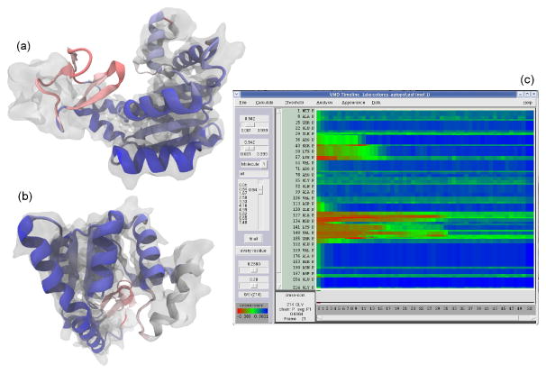
Per-secondary-structure-component local cross correlation of adenylate kinase. MDFF was run on an initial conformation of adenylate kinase (PDB 1AKE) in order to fit it to a simulated density at 5 Å resolution from another conformation (PDB 4AKE). Panels (a) and (b) show a point during the simulation before the structure has been completely fit, colored by per-secondary-structure-component local cross correlation. Darker blue indicates the areas of best fit, while red indicates poorly fitting regions. Panel (a) clearly shows a beta sheet almost completely outside of the reference density and it is colored red to indicate a poor cross correlation. Panel (b) shows a helix partly in the density, and it is colored a very light blue. (c) VMD TimeLine analysis of the cross correlation over the entire simulation. Note how regions of poor fit (red) turn green and blue during the course of the simulation.

The VMD TimeLine trajectory analysis plugin ⁴⁷ makes use of the new data-parallel CPU and GPU quality-of-fit algorithms to provide an interactive visualization of the entire fitting process. TimeLine is designed to help identify and assess trajectory events by performing analysis calculations for each component of a molecular system, and for every frame of a simulation trajectory. The heatmap-style 2-D matrix TimeLine plot provides a “whole-trajectory” and a “whole-structure” view of the calculated property. Figure 1c shows an example plot: the time dimension is displayed horizontally, the structure-component dimension is displayed vertically, and the property of interest – here, density map cross correlation score – is presented by colored rectangles. The TimeLine plot is connected interactively to the VMD 3-D structure display. When the user “scrubs” the mouse cursor around features on the plot, TimeLine highlights the associated 3-D molecular structures and displays their configurations and motions at the times of the corresponding events. A researcher can identify structure transitions, trends, and sequences in a trajectory more quickly by using a single zoomable, interactive 2-D TimeLine plot than by examining a complex 3-D structure over many trajectory frames. When calculating density map cross correlations, different types of trajectory information can be obtained by dividing the system into analysis components of different sizes: fine division among individual residues or contiguous secondary structures (as in Figure 1c) allows detailed structural assessment, while coarser division to fractions of protein segments or even entire protein segments provides information about larger structural elements, particularly for larger systems.

If quality-of-fit analysis can be performed fast enough for interactive updates to keep pace with a running simulation, the correlations can be visualized by the user in real time. Such a real-time analysis can enable the user, along with interactive molecular dynamics (IMD)⁴⁸, to monitor fitting progress and manually manipulate parts of the structure. The user could move the structure in an attempt to improve the correlation while being provided immediate feedback about the resulting effects, with trajectory and local trend context provided by an updating TimeLine view. This technique could make the fitting of difficult structures a much easier process while providing detailed analysis at every step. Additionally, this method could help fit small regions which normally take a long time to fit, often well after most of the structure has long since converged. Interactive MDFF has been performed in the past for studies on the ribosome²⁹, but realtime quality-of-fit analysis could provide for better fits and easier simulations.

4 Methods for Evaluating Quality of Fit

In MDFF, the simulated density is compared to the experimental map using Pearson's correlation coefficient, given by

$${\mathrm{\rho }}_{\mathit{\text{SE}}}=\frac{\langle \left(S-\langle S\rangle \right)\left(E-\langle E\rangle \right)\rangle }{{\mathrm{\sigma }}_S{\mathrm{\sigma }}_E}$$ (3)

where 〈S〉 and 〈E〉 are the average voxel values of the simulated and experimental density maps, respectively, and σ_S and σ_e are their standard deviations⁴⁹. The result is a normalized (ρ_SE∈[−1,1]) indicator of the quality of fit of a given structure in the experimental density. The cross correlation defined in Eq. 3 is traditionally used as a global measure which includes all voxels in the density maps, or as a local correlation¹¹ where only the volume surrounding the molecule is considered. The global correlation is affected by the size of the volume and includes contribution not only from the molecule, but also the solvent. Global correlations can be made artificially higher by considering larger volumes which have been arbitrarily padded. As such, local correlations tend to offer a more useful and unbiased characteristic. In MDFF, local correlations are calculated by specifying a threshold as some number of standard deviations above the mean value of the simulated density. All voxels containing density values lower than this threshold are excluded from the cross correlation calculation. With higher density values naturally occurring closer to the structure, the density being used for the calculation is thus contained within the molecular envelope.

One impediment to creating a fast algorithm for computing the cross correlation is the need for knowledge of the mean value of each map for both the covariance and standard deviations. A simple two-pass algorithm would first iterate through the maps and compute the mean, followed by a second iteration which would compute the covariance and standard deviation. In the interest of speed and efficiency, a single-pass algorithm would be desirable, where only one iteration over the densities would be required. For a single-pass version of the standard deviation calculation, the equation can be rewritten

$${\sigma }_S=\sum _{i=1}^N\frac{1}{N}{\left(x_i-\overline{x}\right)}^2=\frac{1}{N}\sum _{i=1}^N\left(x_i^2-2\overline{x}{x}_i+{\overline{x}}^2\right)=\frac{1}{N}\sum _{i=1}^N{x}_i^2-\frac{2\overline{x}}{N}\sum _{i=1}^N{x}_i+\frac{N{\overline{x}}^2}{N}=(\frac{1}{N}\sum _{i=1}^N{x}_i^2)-2{\overline{x}}^2+{\overline{x}}^2$$ (4)

$${\sigma }_S=(\frac{1}{N}\sum _{i=1}^N{x}_i^2)-{\overline{x}}^2$$ (5)

This expression permits one to compute the sum and the sum of squares of the voxels in each map in a single pass, with the standard deviation being calculated afterwards. This technique can similarly be extended to create a single-pass formulation of covariance. Unfortunately, when the single-pass equations are implemented in floating point arithmetic, they are susceptible to floating point truncation and cancellation error, which can affect the accuracy of the results. Floating point error can be minimized by shifting the means of the reference and simulated maps to zero, and by ensuring that the simulated density maps closely approximate the standard deviation of a reference map, thereby reducing the magnitudes of accumulated squared quantities. Further improvements to floating point precision can be achieved by performing summations in a hierarchical fashion, by using double-precision arithmetic, or through the use of precision enhancement techniques such as Kahan's compensated summation, native-pair arithmetic, and others^50–52. In our tests, we have confirmed the presence of floating error, but even without implementing all of the amelioration techniques described above, we have concluded that the errors have a negligible effect on the final correlation results for the test cases we have run to date. We believe this to be the direct result of a well-conditioned input scenario due to the limited dynamic range of the density values contained within both experimental and simulated density maps.

5 Data-Parallel Cross-Correlation Algorithms

We have devised high-performance data-parallel algorithms for computing simulated density maps, and comparing them with reference density maps using multi-core CPUs with vector instructions and massively parallel GPUs. Each of the methods we have devised for evaluating the quality-of-fit between an all-atom structure and a reference experimental density map requires the computation of a simulated density map from the all-atom structure. Once computed, the simulated density map is then compared with the experimental reference map using voxel-by-voxel subtraction, Pearson correlation, sum of absolute differences, and similar methods. In all of the methods we have evaluated thus far, the generation of the simulated density map is by far the most computationally demanding algorithm step. Since the simulated density value at a given point in space can be computed independently from the values of all other points, the simulated density map computation is well-suited to data-parallel implementations using CPU vector instructions such as the Intel x86 SSE and AVX instructions, or the ARM NEON instructions. Similarly, the computation can take advantage of GPU-accelerated algorithms that employ tens of thousands of threads running on thousands of arithmetic units. Once the simulated density map has been computed, it can be compared with the experimental reference map using a variety of methods.

A key difference between different density map comparison techniques lies in their respective memory capacity requirements and, in the case of GPU implementations, the host-GPU memory transfer characteristics of each algorithm. It is a straightforward task to implement quality-of-fit algorithms using multipass approaches that compute densities, means, and covariances in distinct steps, but these approaches lose performance relative to implementations that combine all steps into a single-pass algorithm. By combining all algorithm steps into a single-pass approach, intermediate values can be stored in fast on-chip registers, shared memory, and caches, that are typically two orders of magnitude faster than accesses to off-chip DRAM. When possible, we employ single-pass cross correlation algorithms, where the simulated density values are computed only ephemerally in CPU or GPU on-chip registers without ever storing the computed density values to off-chip DRAM memory. This approach avoids performance limitations that arise from the roughly factor of 40 performance gap between peak GPU arithmetic throughput (e.g., 2-4.5TFLOPS) and GPU DRAM memory bandwidth (e.g., 200-300 GB/sec).

We have previously developed fast algorithms for calculating and visualizing molecular orbitals present in quantum chemistry calculations⁵³, and for display of molecular surfaces, biomolecular complexes, and cellular structures^54–56. These algorithms each require rapid evaluation of Gaussian radial basis functions, which is also necessary for computation of simulated density maps used in computing cross correlations. In the present work, the simulated density map is computed from a linear combination of Gaussian radial basis functions, with per-atom weighting factor based on atomic radii. The simulated density map can be computed in a single-pass, for single-coefficient atomic weighting factors, or in multiple passes when creating temporally averaged density maps, and to support the use of more sophisticated schemes that use radial basis functions with multiple Gaussian terms or other basis functions. The reference density is tested for exclusion, and the simulated densities are compared with an optional user-defined threshold criterium to determine if they should contribute to the cross correlation. Reference voxels assigned with the IEEE floating point special value NaN (not-a-number), are excluded from consideration. Similarly, simulated density values that fall below an optional user-defined density threshold are also excluded from contributing to the cross correlation. All voxels for which both the reference and simulated densities pass the exclusion and thresholding tests contribute then to the partial sums for the overall cross correlation. When all densities have been processed, a final reduction is performed to compute the final cross correlation from all partial sums that were previously computed.

The new single-pass cross correlation algorithm for GPUs is based on the NVIDIA CUDA programming toolkit⁵⁷, and is referred to hereafter as VMD-GPU-CUDA. The GPU cross correlation algorithm uses a parallel decomposition outlined in Fig. 2. Density contributions from neighboring atoms within the cutoff distance are summed into thread-local registers. The cutoff distance is chosen such that density contributions at or sufficiently near zero are discarded, thereby ensuring that the algorithm achieves linear time complexity. Each thread produces four density values by looping over consecutive densities along the z-axis. Each thread computes its own local contributions to the per-tile cross correlation partial sums, for its four densities according to the voxel exclusion and thresholding criteria described above. Each CUDA thread block performs a local intra-block parallel reduction among all threads, summing each of the thread-local partial sums into a single set of cross-correlation partial sums associated with that block's 8×8×8 tile. Once the intra-block parallel reduction is complete, the first thread of the thread block computes a tile-local cross correlation, and stores both the tile-local cross correlation as well as the per-tile cross correlation partial sums to GPU global memory, in preparation for a final inter-block parallel reduction that yields the overall cross correlation result. One important performance-critical detail about our implementation is that we employ special counters and atomic memory update instructions to allow a single GPU kernel invocation to perform the entire cross correlation calculation. Each thread block increments a global counter using an atomic-add machine instruction as it completes its tile-local work. All but the last thread block to complete simply exit once they have finished their tile-local work. The last thread block to complete its tile-local work performs the final inter-block parallel reduction of all partial sums and stores the overall cross correlation result to GPU global memory.

Fig. 2.

Parallel decomposition for the single-pass GPU-accelerated cross correlation algorithm. The simulated density map is decomposed into 8×8×8 tiles which are processed by individual CUDA thread blocks. Each thread block is 8×8×2 threads in size. Each thread computes 4 consecutive densities along the z–axis, thereby enabling reuse of atom data in on-chip registers and increasing arithmetic throughput. Each CUDA thread block performs thresholding and computes partial sums for the overall cross correlation, as well as the local cross correlation value for its 8×8×8 tile.

The new cross-correlation algorithm for multi-core CPUs employs CPU vector instructions and multithreading. The new CPU algorithm is hereafter referred to as VMD-CPU-SSE. The CPU algorithm decomposes the density map into planar slices which are dynamically assigned to a fixed pool of CPU worker threads by a dynamic load balancer built into VMD⁴⁷. Each CPU worker thread runs a loop that accumulates densities from each onto the region surrounding the atom up to a defined cutoff limit where the Gaussian is assumed to have reached zero. Mainstream multi-core CPUs lack dedicated machine instructions for calculation of exponentials; as a result, application software must either use general purpose math library routines or incorporate custom functions for this purpose. Since the sign of the exponential function's input domain is always negative for the density map synthesis algorithm we have developed, we use a high-performance Taylor series approximation of the exponential function. Our specialized negative-domain exponential approximation is hand-written in assembly language intrinsics for Intel x86 SSE 4-way vector instructions, based on a similar function we originally developed for molecular orbital display⁵³. We have improved the performance of the new exponential approximation beyond what we had previously achieved by premultiplying input values with constants to convert to base-e, and by eliminating conditional tests that check for input domain cases that cannot occur in our density map algorithm, and by guaranteeing multiple-of-four data alignment. The end result of these optimizations is that the multi-core CPU density map algorithm is very competitive with the performance obtained with GPUs, which have machine instructions for computing exponentials due to their heavy use in computer graphics lighting algorithms.

6 Test Cases and Performance Results

In order to test the new data-parallel GPU and CPU cross correlation algorithms, nine test cases were chosen from structures of varying size with density maps at resolutions between 3 Å and 8 Å (Fig. 3, Table 1, Table 2). Six of the structures are final results of MDFF simulations with their corresponding experimental cryo-EM maps, while the remaining three are structures with simulated density maps using the Situs⁴⁰ program pdb2vol⁴¹. The largest structure is the rabbit hemorrhagic disease virus (RHDV) capsid solved with a 6.5 Å resolution density map⁵⁹. Structures of aquaporin, GroEL, GroEL-GroES complex in the ATP-bound state, Mm-cpn in the closed state, and lidless Mm-cpn in the open state, were taken from the results of a cryo-EM modeling challenge⁶⁰. The final structure, ribose binding protein (PDB: 1URP) was used to simulate density maps at 3 Å and 8 Å using Situs, as a means of comparing to density maps generated from another program (Table 1). The size of the virus capsid and the difficult to fit nature of the modeling challenge structures both pose problems to researchers using hybrid fitting methods. Our data-parallel GPU and multi-core CPU cross correlation methods were compared to the previous sequential algorithm in VMD, as well as Chimera⁴², another program widely used by cryo-EM researchers.

Fig. 3.

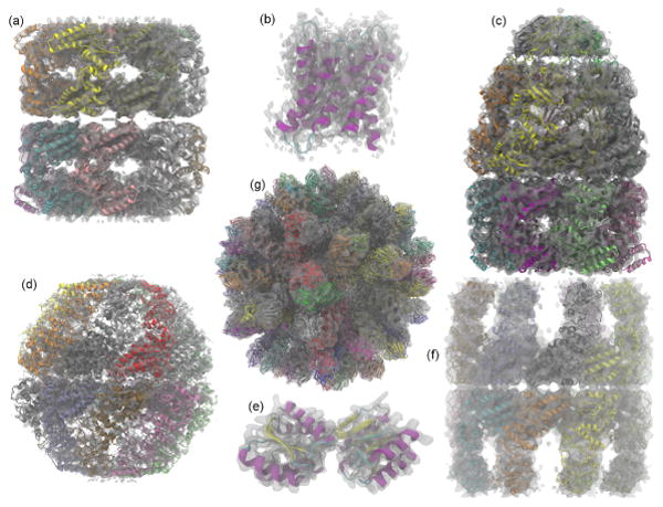
All test systems fitted within their experimental density, or in the case of 1URP, a synthetic one. (a) GroEL PDB 3E76; (b) aquaporin-0 PDB 3M9I; (c) GroEL-GroES complex in the ATP-bound state PDB 2C7D; (d) Mm-cpn in the closed state PDB 3LOS; (e) D-ribose-binding protein PDB 1URP; (f) lidless Mm-cpn in the open state, PDB 3LOS was used as a template to construct a homology model using Modeler⁵⁸; (g) rabbit hemorrhagic disease virus capsid (RHDV) PDB 3J1P.

Table 2.

Comparison of cross correlation algorithm results, runtimes, and speedups for the new GPU and CPU algorithms in VMD, for Chimera, and for the original sequential VMD algorithm. All speedups are normalized using Chimera runtime as the baseline.

	RHDV	Mm-cpn open	GroEL	GroEL-GroES	Mm-cpn closed	Aquaporin
Resolution (Å)	6.5	8	4	7.7	4.3	3
# atoms	702K	61K	54K	59K	64K	1.6K
# voxels	111M	14M	8M	7M	7M	2.6M
VMD-GPU-CUDA cc	0.744	0.857	0.769	0.886	0.658	0.754
VMD-CPU-SSE cc	0.736	0.866	0.839	0.892	0.712	0.771
Chimera cc	0.687	0.837	0.727	0.867	0.635	0.739
VMD-CPU-SEQ cc	0.743	0.869	0.846	0.898	0.728	0.653
VMD-GPU-CUDA	0.458 s 34.6×	0.06 s 25.7×	0.034 s 36.8×	0.038 s 35.0×	0.028 s 57.5×	0.007 s 55.7×
VMD-CPU-SSE	0.779 s 20.3×	0.085 s 18.1×	0.159 s 7.9×	0.077 s 17.3×	0.179 s 9.0×	0.033 s 11.8×
Chimera	15.86 s 1.0×	1.54 s 1.0×	1.25 s 1.0×	1.33 s 1.0×	1.61 s 1.0×	0.39 s 1.0×
VMD-CPU-SEQ	62.89 s 0.25×	2.9 s 0.53×	1.57 s 0.79×	2.49 s 0.53×	2.13 s 0.75×	0.04 s 9.7×

The new VMD cross correlation algorithms provide a significant speedup over both the old sequential CPU code in VMD as well as Chimera, and they provide correlation results that agree with Chimera to within 5% for most cases. In the case where the two have the greatest divergence (7.92% difference), the virus capsid, our method results in a .998 cross correlation with a simulated map produced by Situs, while Chimera reports a correlation of .7842 (Table 1). Because of this discrepancy on the simulated data, we believe that the correlation result for the large capsid reported by Chimera might be flawed, or that it is otherwise not necessarily directly comparable in that specific case.

The new feature for calculating spatial cross correlation maps provides a rapid means of visualizing 3-D correlations and resolving areas of poor fit, as seen in Fig. 4. These spatial correlation maps are especially useful for large complexes, for example virus capsids, because only a single density calculation is required to obtain localized information. By using the VolumeSlice representation in VMD to view 3-D textured slice planes of the correlation map in the x–, y–, or z– axis, the map can be quickly scanned for regions of low correlation. Structure components located in regions of poor correlation can be identified by selecting them or coloring them based on local cross correlation values (Fig. 5).

Fig. 4.

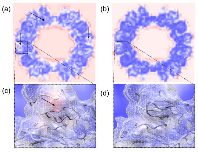
Planar VolumeSlice representation of spatial cross correlation maps for the (a) first and (b) last frames of an MDFF simulation of the rabbit hemorrhhagic disease virus capsid. These maps visualize local cross correlation of 8×8×8 voxel regions, with red indicating poorest correlation and dark blue indicating best correlation. Regions of poorest correlation lie on the exterior and interior faces of the capsid, as would be expected. Poor-fitting regions within the subunits of the structure are seen as red spots and are marked with arrows. Panels (c) and (d) show closer views of one of these poor-fitting regions, before and after fitting, respectively. The structure is shown inside the experimental density map and is colored according to the corresponding spatial cross correlation volume around that region, to further visualize which parts of the structure have a poor fit. Panel (c) clearly shows a poorly fit region, with parts of the structure entirely outside of the density, which has been fixed by MDFF as evident in (d).

Fig. 5.

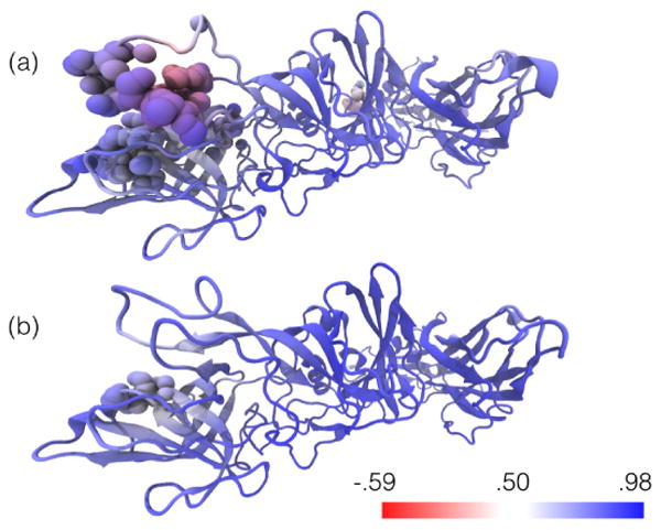
One subunit of the rabbit hemorrhhagic disease virus capsid before (a) and after (b) MDFF. The structure is colored according to the spatial cross correlation volume around that region. A VDW representation shows part of the structure selected as those atoms which lie inside voxels of the spatial cross correlation volume with values < 0.1.

All single-node workstation class tests were run on a workstation containing two Intel Xeon E5-2687W processors each consisting of 8 physical processor cores and 16 hardware threads, for a total of up to 32 threads of execution in hardware. The workstation was configured with 256GB of memory, and an NVIDIA Quadro K6000 GPU with 12GB of on-board memory. All software was run on CentOS Linux version 5.9, and NVIDIA driver version 331.22. VMD was compiled using Intel C/C++ version 12.0.2, and CUDA toolkit version 4.0. Tests involving Situs used Situs version 2.7.1, as obtained from the Situs web site. Chimera tests used version 1.8.1 as obtained from the Chimera web site.

The accelerated cross correlation method makes feasible both detailed and global trajectory assessments of large molecular systems. Figure 6 shows an example of the diagnostic insight provided by a TimeLine view of the initial part of an MDFF simulation of RHDV capsid: 100 frames sampled from a initial 10,000-step energy minimization with MDFF forces active, followed by 400 frames sampled from the initial 40 ps of the MDFF dynamics trajectory. The structure is divided into 180 components: the 180 protein segments, each with an identical residue sequence, that make up the symmetrical virus capsid. In Figure 6a, the pronounced pattern of horizontal stripes indicates a periodic segment-to-segment variation of cross correlation values, following differences in the capsid's symmetrical segment arrangement, as seen in Figure 6b. Figure 6c shows relative changes observed for the individual capsid segments during the trajectory: the trajectory values are normalized by subtracting the initial cross correlation value for each segment. About half of the cross-correlation change seen in Figure 6c occurs during the initial minimization to frame 100, with much of the remaining improvement occuring quickly during the first picoseconds of the MDFF simulation, from frames 100 to 125, and minor fluctuations ceasing for the majority of segments by frame 350. Several segments can be seen to have relatively stable correlation values during both MDFF minimization and MDFF dynamics; a researcher studying the system might investigate these segments further.

Fig. 6.

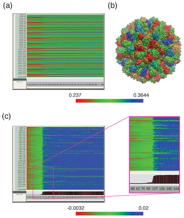
Cross correlation coefficients in an rabbit hemmorrhagic disease virus (RHDV) MDFF trajectory. Panel (a) contains a TimeLine plot of the 500-frame RHDV trajectory discussed in the text, displaying the per-segment cross correlation coefficients. Panel (b) shows the RHDV structure colored by the values in the first frame (right-most column) of panel (a). Panel (c) contains a TimeLine plot of the same trajectory as in panel (a), displaying the change from initial value of per-segment cross correlation, namely, the per-segment values in panel (a) after subtracting the value for each segment in the first frame. The bar graph at the bottom of the plot shows (in brown and black bars at the bottom) the proportion of segments at each timestep with a change in cross correlation greater than +0.01.

Detailed analysis of very large systems with long trajectories can require a large number of individual calculations, and impose a heavy I/O burden on a compute system. We implemented a parallel TimeLine cross correlation analysis using the new GPU cross correlation algorithm, for use on clusters or supercomputers. The new TimeLine analysis calls call VMD parallel scripting primitives⁴⁷ to perform the needed calculation, synchronization, and data reduction operations. A 10,000 frame trajectory of the 1.38 million atom RHDV capsid structure was examined. For cross correlation analysis, the capsid was divided into 720 structural components; each of the capsid's 180 525-residue segments were divided into four nearly-equal contiguous segments. The calculation was run on the NSF Blue Waters petascale supercomputer, using the XK7 hybdrid GPU-accelerated compute nodes. Each XK7 node contains an AMD Opteron 6276 CPU with 32GB of RAM and an NVIDIA Tesla K20X GPU accelerator with 6 GB of RAM. Structure and trajectory files were striped over 160 Lustre file system object storage targets to ensure best I/O performance⁴⁷. The analysis completed in 3.2 hours using 128 nodes, showing a 105× speedup over the projected 336.2 hour (14.0 day) runtime using a single node. Using the Table 2 performance results, this would roughly correspond to a 3,649× speedup over an estimated 485 day (1.3 year) runtime for Chimera running on a single node and a 14,471× speedup over an estimated 1,924 day (5.3 year) runtime for the original sequential VMD CPU algorithm running on a single node.

7 Conclusions

We have presented data-parallel cross correlation algorithms that combine density map synthesis, computation of spatial cross correlation maps, and overall cross correlation between the synthetic and reference density maps, using a high performance single-pass approach on multi-core CPUs using SSE vector instructions, and on massively parallel GPUs using CUDA. The new algorithms achieve significant speedups compared to existing methods and they maintain adequate numerical precision. The single-pass algorithms achieve high performance by fusing independent algorithm steps into a single computational kernel, thereby maximizing the ratio of arithmetic operations vs. memory references, which is of greatest overall benefit to massively parallel GPU hardware. We have demonstrated the use of the new algorithms in several visualization and analysis contexts over a range of problem sizes, and have incorporated that high performance cross correlation method into a TimeLine multi-node parallel analysis script enabling large systems and long trajectories to be analyzed rapidly on clusters or supercomputers. We expect that with further algorithm development, the performance of the new cross correlation algorithm can still be improved further. New data-parallel shuffle instructions available on recent NVIDIA GPUs could be used to accelerate the intra-block and inter-block parallel reductions that take place within the GPU algorithm. The most recent Intel and AMD processors have added new 8-element AVX and AVX2 vector instructions, offering up to a 2× performance gain over SSE instructions. The greatly increased performance levels achieved by the new algorithms create many new opportunities for interactive analyses and visualizations and for interactive molecular dynamics simulations⁴⁸ using the MDFF method.

References

- 1.Zhao G, Perilla JR, Yufenyuy EL, Meng X, Chen B, Ning J, Ahn J, Gronenborn AM, Schulten K, Aiken C, Zhang P. Nature. 2013;497:643–646. doi: 10.1038/nature12162. [DOI] [PMC free article] [PubMed] [Google Scholar]
- 2.Zhang J, Baker ML, Schröder GF, Douglas NR, Reissmann S, Jakana J, Dougherty M, Fu CJ, Levitt M, Ludtke SJ, Frydman J, Chiu W. Nature. 2010;463:379–383. doi: 10.1038/nature08701. [DOI] [PMC free article] [PubMed] [Google Scholar]
- 3.Ludtke SJ, Baker ML, Chen DH, Song JL, Chuang DT, Chiu W. Structure. 2008;16:441–448. doi: 10.1016/j.str.2008.02.007. [DOI] [PubMed] [Google Scholar]
- 4.Zhang X, Settembre E, Xu C, Dormitzer PR, Bellamy R, Harrison SC, Grigorieff N. Proc Natl Acad Sci USA. 2008;105:1867–1872. doi: 10.1073/pnas.0711623105. [DOI] [PMC free article] [PubMed] [Google Scholar]
- 5.Baker ML, Zhang J, Ludtke SJ, Chiu W. Nat Protoc. 2010;5:1697–1708. doi: 10.1038/nprot.2010.126. [DOI] [PMC free article] [PubMed] [Google Scholar]
- 6.Hryc CF, Chen DH, Chiu W. Curr Opin Virol. 2011;1:110–117. doi: 10.1016/j.coviro.2011.05.019. [DOI] [PMC free article] [PubMed] [Google Scholar]
- 7.Zhang R, Hryc CF, Cong Y, Liu X, Jakana J, Gorchakov R, Baker ML, Weaver SC, Chiu W. EMBO J. 2011;30:3854–3863. doi: 10.1038/emboj.2011.261. [DOI] [PMC free article] [PubMed] [Google Scholar]
- 8.Maki-Yonekura S, Yonekura K, Namba K. Nat Struct Mol Biol. 2010;17:417–422. doi: 10.1038/nsmb.1774. [DOI] [PubMed] [Google Scholar]
- 9.Cheng L, Zhu J, Hui WH, Zhang Z, Honig B, Fang Q, Zhou ZH. J Mol Biol. 2010;397:852–863. doi: 10.1016/j.jmb.2009.12.027. [DOI] [PMC free article] [PubMed] [Google Scholar]
- 10.Fabiola F, Chapman MS. Structure. 2005;13:389–400. doi: 10.1016/j.str.2005.01.007. [DOI] [PubMed] [Google Scholar]
- 11.Roseman AM. Acta Cryst D. 2000;56:1332–1340. doi: 10.1107/s0907444900010908. [DOI] [PubMed] [Google Scholar]
- 12.Das R, Baker D. Annu Rev Biochem. 2008;77:363–382. doi: 10.1146/annurev.biochem.77.062906.171838. [DOI] [PubMed] [Google Scholar]
- 13.Schröder GF, Brunger AT, Levitt M. Structure. 2007;15:1630–1641. doi: 10.1016/j.str.2007.09.021. [DOI] [PMC free article] [PubMed] [Google Scholar]
- 14.Jolley CC, Wells SA, Fromme P, Thorpe MF. Biophys J. 2008;94:1613–1621. doi: 10.1529/biophysj.107.115949. [DOI] [PMC free article] [PubMed] [Google Scholar]
- 15.Tama F, Miyashita O, Brooks CL., III J Struct Biol. 2004;147:315–326. doi: 10.1016/j.jsb.2004.03.002. [DOI] [PubMed] [Google Scholar]
- 16.Orzechowski M, Tama F. Biophys J. 2008;95:5692–5705. doi: 10.1529/biophysj.108.139451. [DOI] [PMC free article] [PubMed] [Google Scholar]
- 17.Chapman MS, Trzynka A, Chapman BK. J Struct Biol. 2013;182:10–21. doi: 10.1016/j.jsb.2013.01.003. [DOI] [PMC free article] [PubMed] [Google Scholar]
- 18.Topf M, Lasker K, Webb B, Wolfson H, Chiu W, Sali A. Structure. 2008;16:295–307. doi: 10.1016/j.str.2007.11.016. [DOI] [PMC free article] [PubMed] [Google Scholar]
- 19.Trabuco LG, Villa E, Mitra K, Frank J, Schulten K. Structure. 2008;16:673–683. doi: 10.1016/j.str.2008.03.005. [DOI] [PMC free article] [PubMed] [Google Scholar]
- 20.Trabuco LG, Villa E, Schreiner E, Harrison CB, Schulten K. Methods. 2009;49:174–180. doi: 10.1016/j.ymeth.2009.04.005. [DOI] [PMC free article] [PubMed] [Google Scholar]
- 21.Phillips JC, Braun R, Wang W, Gumbart J, Tajkhorshid E, Villa E, Chipot C, Skeel RD, Kale L, Schulten K. J Comp Chem. 2005;26:1781–1802. doi: 10.1002/jcc.20289. [DOI] [PMC free article] [PubMed] [Google Scholar]
- 22.Wells D, Abramkina V, Aksimentiev A. J Chem Phys. 2007;127:125101–125101–10. doi: 10.1063/1.2770738. [DOI] [PMC free article] [PubMed] [Google Scholar]
- 23.Schreiner E, Trabuco LG, Freddolino PL, Schulten K. BMC Bioinform. 2011;12:190. doi: 10.1186/1471-2105-12-190. [DOI] [PMC free article] [PubMed] [Google Scholar]
- 24.Chan KY, Gumbart J, McGreevy R, Watermeyer JM, Sewell BT, Schulten K. Structure. 2011;19:1211–1218. doi: 10.1016/j.str.2011.07.017. [DOI] [PMC free article] [PubMed] [Google Scholar]
- 25.Villa E, Sengupta J, Trabuco LG, LeBarron J, Baxter WT, Shaikh TR, Grassucci RA, Nissen P, Ehrenberg M, Schulten K, Frank J. Proc Natl Acad Sci USA. 2009;106:1063–1068. doi: 10.1073/pnas.0811370106. [DOI] [PMC free article] [PubMed] [Google Scholar]
- 26.Gumbart J, Trabuco LG, Schreiner E, Villa E, Schulten K. Structure. 2009;17:1453–1464. doi: 10.1016/j.str.2009.09.010. [DOI] [PMC free article] [PubMed] [Google Scholar]
- 27.Becker T, Bhushan S, Jarasch A, Armache JP, Funes S, Jossinet F, Gumbart J, Mielke T, Berninghausen O, Schulten K, Westhof E, Gilmore R, Mandon EC, Beckmann R. Science. 2009;326:1369–1373. doi: 10.1126/science.1178535. [DOI] [PMC free article] [PubMed] [Google Scholar]
- 28.Seidelt B, Innis CA, Wilson DN, Gartmann M, Armache JP, Villa E, Trabuco LG, Becker T, Mielke T, Schulten K, Steitz TA, Beckmann R. Science. 2009;326:1412–1415. doi: 10.1126/science.1177662. [DOI] [PMC free article] [PubMed] [Google Scholar]
- 29.Trabuco LG, Schreiner E, Eargle J, Cornish P, Ha T, Luthey-Schulten Z, Schulten K. J Mol Biol. 2010;402:741–760. doi: 10.1016/j.jmb.2010.07.056. [DOI] [PMC free article] [PubMed] [Google Scholar]
- 30.Gumbart J, Schreiner E, Trabuco LG, Chan KY, Schulten K. Molecular Machines in Biology. ch. 8. Cambridge University Press; 2011. pp. 142–157. [Google Scholar]
- 31.Frauenfeld J, Gumbart J, van der Sluis EO, Funes S, Gartmann M, Beatrix B, Mielke T, Berninghausen O, Becker T, Schulten K, Beckmann R. Nat Struct Mol Biol. 2011;18:614–621. doi: 10.1038/nsmb.2026. [DOI] [PMC free article] [PubMed] [Google Scholar]
- 32.Agirrezabala X, Schreiner E, Trabuco LG, Lei J, Ortiz-Meoz RF, Schulten K, Green R, Frank J. EMBO J. 2011;30:1497–1507. doi: 10.1038/emboj.2011.58. [DOI] [PMC free article] [PubMed] [Google Scholar]
- 33.Li W, Trabuco LG, Schulten K, Frank J. Proteins: Struct, Func, Bioinf. 2011;79:1478–1486. doi: 10.1002/prot.22976. [DOI] [PMC free article] [PubMed] [Google Scholar]
- 34.Hsin J, Gumbart J, Trabuco LG, Villa E, Qian P, Hunter CN, Schulten K. Biophys J. 2009;97:321–329. doi: 10.1016/j.bpj.2009.04.031. [DOI] [PMC free article] [PubMed] [Google Scholar]
- 35.Sener MK, Hsin J, Trabuco LG, Villa E, Qian P, Hunter CN, Schulten K. Chem Phys. 2009;357:188–197. doi: 10.1016/j.chemphys.2009.01.003. [DOI] [PMC free article] [PubMed] [Google Scholar]
- 36.Vasishtan D, Topf M. J Struct Biol. 2011;174:333–343. doi: 10.1016/j.jsb.2011.01.012. [DOI] [PubMed] [Google Scholar]
- 37.Diamond R. Acta Cryst A. 1971;27:436–452. [Google Scholar]
- 38.Jones TA, Liljas L. Acta Cryst A. 1984;40:50–57. [Google Scholar]
- 39.Stewart PL, Fuller SD, Burnett RM. EMBO J. 1993;12:2589–2599. doi: 10.1002/j.1460-2075.1993.tb05919.x. [DOI] [PMC free article] [PubMed] [Google Scholar]
- 40.Wriggers W. Biophysical Reviews. 2010;2:21–27. doi: 10.1007/s12551-009-0026-3. [DOI] [PMC free article] [PubMed] [Google Scholar]
- 41.Wriggers W. Acta Cryst D. 2012;68:344–351. doi: 10.1107/S0907444911049791. [DOI] [PMC free article] [PubMed] [Google Scholar]
- 42.Pettersen EF, Goddard TD, Huang CC, Couch GS, Greenblatt DM, Meng EC, Ferrin TE. J Comp Chem. 2004;25:1605–1612. doi: 10.1002/jcc.20084. [DOI] [PubMed] [Google Scholar]
- 43.Ludtke SJ, Baldwin PR, Chiu W. J Struct Biol. 1999;128:82–97. doi: 10.1006/jsbi.1999.4174. [DOI] [PubMed] [Google Scholar]
- 44.Chapman MS. Acta Cryst A. 1995;51:69–80. [Google Scholar]
- 45.Chacón P, Wriggers W. J Mol Biol. 2002;317:375–384. doi: 10.1006/jmbi.2002.5438. [DOI] [PubMed] [Google Scholar]
- 46.Humphrey W, Dalke A, Schulten K. J Mol Graphics. 1996;14:33–38. doi: 10.1016/0263-7855(96)00018-5. [DOI] [PubMed] [Google Scholar]
- 47.Stone JE, Isralewitz B, Schulten K. Proceedings of the XSEDE Extreme Scaling Workshop. 2013 [Google Scholar]
- 48.Stone JE, Gullingsrud J, Grayson P, Schulten K. 2001 ACM Symposium on Interactive 3D Graphics; New York. 2001. pp. 191–194. [Google Scholar]
- 49.Frank J. Three-dimensional electron microscopy of macromolecular assemblies. Oxford University Press; New York: 2006. [Google Scholar]
- 50.Kahan W. Commun ACM. 1965;8:40. [Google Scholar]
- 51.He Y, Ding CHQ. ICS '00: Proceedings of the 14th international conference on Super-computing; New York, NY, USA. 2000. pp. 225–234. [Google Scholar]
- 52.Bailey DH. Comput in Sci and Eng. 2005;07:54–61. [Google Scholar]
- 53.Stone JE, Saam J, Hardy DJ, Vandivort KL, Hwu WW, Schulten K. Proceedings of the 2nd Workshop on General-Purpose Processing on Graphics Processing Units, ACM International Conference Proceeding Series; New York, NY, USA. 2009. pp. 9–18. [Google Scholar]
- 54.Krone M, Stone JE, Ertl T, Schulten K. EuroVis - Short Papers 2012. 2012:67–71. [Google Scholar]
- 55.Roberts E, Stone JE, Luthey-Schulten Z. J Comp Chem. 2013;34:245–255. doi: 10.1002/jcc.23130. [DOI] [PMC free article] [PubMed] [Google Scholar]
- 56.Stone JE, Vandivort KL, Schulten K. Proceedings of the 8th International Workshop on Ultrascale Visualization; New York, NY, USA. 2013. pp. 6:1–6:8. [Google Scholar]
- 57.Nickolls J, Buck I, Garland M, Skadron K. ACM Queue. 2008;6:40–53. [Google Scholar]
- 58.Sali A, Blundell TL. J Mol Biol. 1993;234:779. doi: 10.1006/jmbi.1993.1626. [DOI] [PubMed] [Google Scholar]
- 59.Wang X, Xu F, Liu J, Gao B, Liu Y, Zhai Y, Ma J, Zhang K, Baker TS, Schulten K, Zheng D, Pang H, Sun F. PLoS Pathog. 2013;9:e1003132. doi: 10.1371/journal.ppat.1003132. [DOI] [PMC free article] [PubMed] [Google Scholar]
- 60.Chan KY, Trabuco LG, Schreiner E, Schulten K. Biopolymers. 2012;97:678–686. doi: 10.1002/bip.22042. [DOI] [PMC free article] [PubMed] [Google Scholar]