

Abstract
Detecting positive selection in species with heterogeneous habitats and complex demography is notoriously difficult and prone to statistical biases. The model plant Arabidopsis thaliana exemplifies this problem: In spite of the large amounts of data, little evidence for classic selective sweeps has been found. Moreover, many aspects of the demography are unclear, which makes it hard to judge whether the few signals are indeed signs of selection, or false positives caused by demographic events. Here, we focus on Swedish A. thaliana and we find that the demography can be approximated as a two-population model. Careful analysis of the data shows that such a two island model is characterized by a very old split time that significantly predates the last glacial maximum followed by secondary contact with strong migration. We evaluate selection based on this demography and find that this secondary contact model strongly affects the power to detect sweeps. Moreover, it affects the power differently for northern Sweden (more false positives) as compared with southern Sweden (more false negatives). However, even when the demographic history is accounted for, sweep signals in northern Sweden are stronger than in southern Sweden, with little or no positional overlap. Further simulations including the complex demography and selection confirm that this is not compatible with global selection acting on both populations, and thus can be taken as evidence for local selection within subpopulations of Swedish A. thaliana. This study demonstrates the necessity of combining demographic analyses and sweep scans for the detection of selection, particularly when selection acts predominantly local.
Keywords: local adaptation, selective sweeps, demography, Arabidopsis thaliana
Introduction
Arabidopsis thaliana is the model organism for plant genetics, at least partly due to the wealth of natural phenotypic variation (Koornneef et al. 2004). Many of these variable traits have been studied in great detail, and the underlying genes have been mapped using crosses and association studies (Atwell et al. 2010). The variation in many of these traits, such as pathogen resistance or flowering time, is unlikely to be selectively neutral. One striking example is variation in the need for vernalization, a period of low temperature required before flowering. This variation reflects the requirement to precisely time flowering in different latitudes, for example, to accommodate the short growing season in the North. Indeed, variants of the FRIGIDA gene match a latitudinal gradient across Europe (Corre et al. 2002), providing evidence for selection using a “top-down” approach starting with the phenotype. In contrast, bottom-up approaches, screens for selective sweeps to identify molecular signatures of selection in A. thaliana, have yielded surprisingly few regions (Clark et al. 2007; Horton et al. 2012). This result stands in contrast to those from species with less population structure, such as Drosophila simulans and melanogaster, which show distinctive patterns of recurrent selective sweeps (Wright and Andolfatto 2008; Sattath et al. 2011).
The same conclusion is reached from a McDonald–Kreitman approach, which quantifies adaptive fixations along a phylogenetic lineage: Little or no evidence for selection in A. thaliana (Bustamante et al. 2002; Gossmann et al. 2010; Slotte et al. 2011) contrasts with high estimates of the fraction of adaptive nucleotide substitutions in Drosophila (Eyre-Walker and Keightley 2009), Mice (Halligan et al. 2010), Humans (Boyko et al. 2008), and Capsella (Slotte et al. 2010), ranging from 20% to 60%. Even more surprisingly, A. thaliana appears to have a slight excess of nonsynonymous polymorphisms, resulting in negative estimates of the rate of adaptation (e.g., for chromosome 3 in Slotte et al. 2011).
Both a lack of global sweep signals and the excess of nonsynonymous polymorphisms are expected under a model of predominantly local adaptation. Indeed, evidence is accumulating that A. thaliana shows adaptation to its local environments (Rutter and Fenster 2007; Fournier-Level et al. 2011; Hancock et al. 2011; Ågren and Schemske 2012; Ågren et al. 2013). This scenario makes intuitive sense: A. thaliana has successfully spread to vastly different environments in a very short time, and the structured genetic diversity across this range suggests that locally adapted variants are likely to exist (Gaut 2012).
So far, evidence for local selection has mainly been found from correlations to environmental variation (e.g., Hancock et al. 2011). However, this means that the environmental factors that lead to adaptation must be known and measurable. In contrast, it is the appeal of a purely genomic bottom-up approach that such prior knowledge is not required. Here, we analyze high-quality whole-genome sequencing data from northern and southern Swedish A. thaliana as published in Long et al. (2013). This data set is promising for the investigation of local selection: Many plants were sampled within a small geographic region (130 in southern Sweden, 50 in northern Sweden), and especially for the northern Swedish population, we can assume that the most relevant aspects of the environment, such as vegetation time, day length, and temperature profile, are homogeneous within the sample.
Long et al. (2013) have used several methods to scan for selective sweeps in both northern and southern Sweden. Based on a scan to detect sweep-like deviations in the site frequency spectrum (SweepFinder), they found strong signals of selective sweeps in northern Sweden, but almost none in southern Sweden. However, no explicit modeling of the complex demography was done, and although SweepFinder is assumed to be robust to many deviations from the standard neutral model, demography still affects the false positive rate (Pavlidis et al. 2008).
In this study, we estimate a model of the demography of Swedish A. thaliana and calculate false positive and negative rates caused by the demography, which we then use to assess the power to detect selection in general and also whether we can distinguish between global and local selection. Our results provide an explanation for the surprising selection patterns of sweeps in northern but not southern Sweden found in Long et al. (2013).
Results
Population Structure of Swedish A. thaliana
Two Populations
The northern Swedish population of A. thaliana shows strong genetic differentiation from other European populations (Nordborg et al. 2005; François et al. 2008; Horton et al. 2012; Long et al. 2013). Therefore previous studies treated “North” and “South” as two separate, panmictic populations (François et al. 2008; Long et al. 2013). Alternatively, one could fit a model of isolation by distance or a more complicated range expansion model, and we explore these options in the following. We started by looking at the correlation between genetic and physical distance in northern and southern Sweden separately, using a stepping stone model of isolation by distance. This model predicts a log-linear relationship between the two distance measures, which is what we observe (supplementary fig. S2, Supplementary Material online). The slopes for northern and southern Sweden are different (0.11% vs. 0.05% per log10 [distance in km], respectively), and the genetic distance between two northern plants is lower than the distance between southern plants in the range of observed physical sampling distances. This suggests that northern Sweden has a lower effective population size (Watterson’s estimate of synonymous diversity: ), and that the northern and the southern Swedish population are distinct.
Removing Substructure
Next, we assessed the scale of physical distance that is responsible for the isolation by distance pattern. By far the strongest contribution comes from plants that were sampled within 2 km of one another. These plants are close to being clonal () in either population. Based on a separation of time scales argument (Nordborg and Donnelly 1997), we decided to choose only one representative sample within a 2 km radius. As it turns out, this strategy removes most substructure also at the genetic level, as can be seen in the principal component analysis (PCA)-analysis (fig. 1) and the comparison of genetic and physical distance (supplementary fig. S3, Supplementary Material online). After this subsampling, the only remaining substructure is a cluster of closely related southern Swedish plants. Closer inspection reveals that they are all located along a major road. We therefore picked only one line from this cluster for further analysis. The resulting subsample of 16 northern and 41 southern Swedish plants is by in large consistent with a two island model. Nevertheless, also more complex models that capture the genetic distance between South and North as well as the isolation by distance within either population can be consistent with the observed patterns. Therefore, we evaluated how well different kinds of linear stepping stone and range expansion models recapitulate the observed summary statistics in both populations (Tajima’s D, Fay and Wu’s H, nucleotide diversity, FST, supplementary table S2, Supplementary Material online). Only in one instance did a more complex model fit equally well as a two-deme model—a model of ten demes in a linear arrangement with our samples as the end populations, and with an asymmetric migration rate favoring migration from North to South forward in time. However, the slight improvement in the fit hardly justifies the added complexity due to the ghost demes. We therefore decided to apply a two-deme framework to the appropriately subsampled data set.
Fig. 1.

Geographical position of plants on a map of Sweden and PCA plot of the first two principal coordinates. A subcluster of 25 closely related plants in southern Sweden is encircled by an ellipse.
Modeling the Long-Term Demographic History of Swedish A. thaliana
Demographic Models
Within the two-deme framework, we modeled a number of potential evolutionary histories. All models begin with the split of the ancestral population and allow for the exchange of migrants. We allow for variable and asymmetric migration, secondary contact after a phase of separation, different deme sizes, population size changes (including bottlenecks) either at the split time or afterwards, and variable split times from the common ancestor. In addition, we model three different admixture scenarios in order to simulate two postglacial waves of expansion (François et al. 2008). In total, we tested 14 models with 4–9 parameters using (Gutenkunst et al. 2009). A summary of the tested models is given in table 1 and figure 2.
Table 1.
—Parameter Estimates for Different Models.
| Model Name | No. | AIC | N0 | T1 | T2 | T3 | Growth | ||||||||||
|---|---|---|---|---|---|---|---|---|---|---|---|---|---|---|---|---|---|
| splitSymMig4 | 4 | 4,085 | 29,000 | 568,000 | 0.41 | 5.66 | 1.67 | ||||||||||
| splitMig5 | 5 | 2,896 | 25,000 | 498,000 | 0.19 | 1.21 | 8.00 | 0.74 | |||||||||
| secondaryContact6 | 6 | 2,609 | 124,000 | 153,000 | 39,000 | =0 | =0 | 1.23 | 5.90 | 1.66 | 0.17 | ||||||
| splitMigBottleneck7 | 7 | 3,019 | 47,000 | 433,000 | 63,000 | 0.45 | 2.15 | 3.73 | 198 | 0.41 | |||||||
| splitMigBottleneck8 | 8 | 2,737 | 92,000 | 310,000 | 34,000 | 19,000 | 0.61 | 4.72 | 2.17 | 0.23 | 0.08 | =NN1 | |||||
| splitMigBottleneck9 | 9 | 2,791 | 45,000 | 470,000 | 45,000 | 0.42 | 1.91 | 2.74 | 4.10 | 4.75 | 0.21 | 0.59 | S&N | ||||
| splitMigGrowth7 | 7 | 3,012 | 23,000 | 467,000 | 0.17 | 1.24 | 26.50 | 7.49 | 0.05 | 0.79 | S&N | ||||||
| splitMigRecentGrowth7 | 7 | 4,395 | 51,000 | 358,000 | 14,000 | 0.37 | 2.05 | 3.22 | 200 | 0.41 | S | ||||||
| secondaryContact- | |||||||||||||||||
| RecentGrowth7 | 7 | 2,772 | 125,000 | 154,000 | 34,000 | =0 | =0 | 1.40 | 6.19 | 1.89 | 1.20 | 0.17 | S | ||||
| splitMigRecentGrowth8 | 8 | 4,644 | 97,000 | 216,000 | 14,000 | 0.62 | 4.19 | 1.72 | 196 | 0.17 | 0.26 | S&N | |||||
| secondaryContact- | |||||||||||||||||
| RecentGrowth8 | 8 | 2,852 | 132,000 | 132,000 | 20,000 | =0 | =0 | 2.44 | 8.39 | 1.66 | 1.03 | 0.32 | 0.09 | S&N | |||
| splitAdmixture5-1a | 5 | 7,080 | 153,000 | 20,000 | 19,000 | =0 | =0 | 0.75b | =0 | 2.88 | 0.16 | ||||||
| splitAdmixture5-2c | 5 | 6,018 | 154,000 | 33,000 | 8,000 | =0 | =0 | 0.90b | =0 | 1.61 | 0.25 | ||||||
| splitAdmixture9d | 9 | 2,768 | 132,000 | 130,000 | 11,470 | 11,410e | 0.07 | 10.69 | 1.25 | 0.10 | |||||||
Note.—Parameters are defined according to (fig. 2a). Times are given in years, population sizes in units of N0 and migration rates in units of . Note that the model-acronym refers to the number of parameters, that is, secondaryContact6 is a 6 parameter model.
aSouthern Sweden appears at time T2 as admixture between northern Sweden and an additional ancestral (unsampled) population.
bValues are admixture proportions instead of migration rates.
cThe admixture event as a pulse of migrating northern Swedish plants to southern Sweden at T2.
dModel with three demes, for details see supplementary figure S10, Supplementary Material online.
eTime of the admixture of middle European plants into southern Sweden.
Fig. 2.

Model diagrams. (a) General model setup. (b) Model scheme and parameter estimates of backward migration rates , times (in units of ) and population sizes (in units of N0) for the best fitting model (secondaryContact6).
The model fit was evaluated using the Akaike information criterion (AIC). All models with AIC <4,000 achieved a good fit to the observed joint Site Frequency Spectrum (jSFS) (supplementary fig. S5, Supplementary Material online). All models slightly underestimate the number of low-frequency alleles. This discrepancy cannot be explained by sequencing errors, as the problem remains also if no singletons are used for inference. Furthermore, this issue persists independently of whether we use whole-genome data or only synonymous sites, so it is unlikely to be due to negative selection. The lowest AIC score was achieved by a model that is characterized by a period of complete isolation between the two populations, with migration only resuming fairly recently (secondaryContact6). The third, fourth, and fifth best models share this property. The model with the second best fit (splitMigBottleneck8) is characterized by a recent extended, but mild, bottleneck in the northern Swedish population. We chose three models for in depth analyses: 1) the best fitting model (secondaryContact6), 2) the second best fitting model (splitMigBottleneck8), because bottlenecks are expected in expanding populations and can potentially create sweep-like patterns of diversity, and 3) a simple but fairly well-fitting isolation-with-migration model (splitMig5), which is the same as the secondary contact model without the separation phase.
Model Fit
We used a parametric bootstrap approach to compare the model fits more rigorously (see Materials and Methods). The results indicate that the likelihood of the secondary contact model given our data is significantly better than expected for data simulated under either the simple isolation-with-migration model or the more complex bottleneck model (see table 2). The bottleneck model only shows marginally significant improvement over the isolation-with-migration model (P = 0.05) but does not improve over the secondary contact model (P = 0.87). These results show that there is statistical support for the secondary contact model (secondaryContact6).
Table 2.
P Values for Model Comparison Based on Parametric Bootstrapping.
| Null Model | Alternative Model |
||
|---|---|---|---|
| splitMig5 | Secondary- Contact6 | splitMig- Bottleneck8 | |
| splitMig5 | — | <0.01 | 0.05 |
| secondaryContact6 | 0.96 | — | 0.87 |
| splitMigBottleneck8 | 0.75 | <0.01 | — |
Additional evidence in support of this model comes from comparing linkage disequilibrium (LD) between the data and coalescent simulations under the secondaryContact6 demography. This model recapitulates the ratio of LD between South and North very well (fig. 3): The estimated population recombination rate is 7.9-fold larger in southern Sweden than in northern Sweden and the simulations predict a comparable ratio of 8.3. For this reason, all subsequent simulation results are based on the secondary contact model.
Fig. 3.
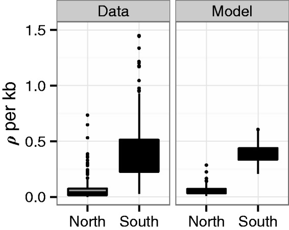
Population recombination rates for the data and the model. ρ is estimated in 1-Mb windows by fitting a curve to the decay of r2 with distance according to Hill and Weir (1988). On average, there is an about 8-fold smaller effective recombination rate in northern compared with southern Sweden in the data. Simulations from the secondaryContact6 model predict a similar ratio.
Although the exact parameter estimates for population split time, migration and population sizes depend on model specifications, there are some properties that hold for all scenarios evaluated (fig. 4): First, the estimated population split time is older than 100 kya. The best estimate for the secondaryContact6 model dates the split to 153 kya, which is amongst the most recent dates estimated from the different models. This split time clearly predates the colonization of Scandinavia (François et al. 2008), as well as the last glacial maximum 18–20 kya (Taberlet et al. 1998), even if we take the lower bounds of the diffusion estimates from and the upper bound for mutation rate of (Ossowski et al. 2010). Excluding the 22 sweep regions of Long et al. (2013) leads to an even larger estimated of the split time (supplementary table S4, Supplementary Material online). Previous estimates of the split time between northern Sweden and southern Sweden arrived at a recent value of no more than 13,500 years (François et al. 2008), which is clearly inconsistent with our results. Indeed, the log-likelihood (LL) of our data given the François model is much lower than for any of our models (LL [François-model]=−35,491 versus LL [secondaryContact6]= −2,597).
Fig. 4.

Point estimates and confidence intervals of robust parameters. (a) Split time between northern Sweden and southern Sweden in generations (with mutation rate μ = 7 × 10⁻⁹ per bp per generation, Ossowski et al. 2010), (b) ratio of current population sizes (South over North), and (c) migration rate from South to North over North to South (forward in time), for fitted models with AIC < 4,000. If no confidence intervals are shown they were not calculable.
Second, the current size of the southern Swedish population is about 7–11-fold larger than that of northern Sweden. Models that allow for exponential growth estimate even higher ratios, but this is likely an artifact because it co-occurs with unreasonably strong growth in the southern population.
Finally, the backwards migration rate of our models is between 3 and 7 times larger for South to North than for the opposite direction. Backwards migration rates can be thought of as the fraction of foreign immigrants per generation, thus if we pick a random plant from the North, we stand a higher chance to pick a migrant from the South than the other way round. To determine how many seeds or plants actually move between the populations, we have to rescale with the relevant population size, which translates to twice as many migrants going from North to South than vice versa.
We were also wondering in how far our ignorance of other neighboring A. thaliana populations could influence the parameter estimates. Ghost demes can bias migration rate and population size estimates if the migration rate from the ghost deme to the sampled demes is large (Beerli 2004; Slatkin 2005). Here, it is easy to imagine that the southern Swedish population receives many immigrants from mainland Europe. We tested several models that include ghost demes, of which the best fitting one is signified by an admixture event of the ghost deme into southern Sweden (splitAdmixture9; supplementary fig. S10, Supplementary Material online). There is little change in split time or population size estimates compared with our best fitting model (fig. 4). However, admixture from a ghost deme might explain the strong support for asymmetric migration in our two-deme models.
Impact of A. thaliana Demography on SweepFinder Composite Likelihood Ratio Distributions
Long et al. (2013) used the program SweepFinder (Nielsen et al. 2005) to look for evidence of recent selective sweeps in A. thaliana. They found evidence for selective sweeps in northern, but not in southern Sweden. The absence of evidence for strong selection in the South is puzzling because we would expect to have more power to detect selection in southern Sweden due to the larger population size relative to the North. In the absence of a detailed demography for this initial sweep scan, Long et al. (2013) determined the critical values for the composite likelihood ratios (CLR) of SweepFinder using the standard neutral model. Although this approach has been found to be conservative for many demographic scenarios (Nielsen et al. 2005), it has never been tested for a secondary contact scenario. Therefore, we explored the effects of demography on CLR distributions in more detail.
We determine the neutral CLR distribution for northern and southern Sweden under the best-fitting demographic model (secondaryContact6). As it turns out, this model mimics the observed shifts in the CLR distribution that we observed for northern and southern Sweden (fig. 5), with the distribution for the North being more skewed and having a higher median than that for the South (table 3). The strong skew in our model is a consequence of the secondary contact scenario: Neither a 100-fold increase in migration, that is, a quasi-panmictic population, where CLR-differences must be due to sample size, nor a scenario without migration can produce a long tail similar to the observed one (supplementary fig. S7, Supplementary Material online). Similar shifts in the CLR distribution, although not as pronounced, were also observed for the two other models we tested: splitMig5 and splitMigBottleneck8 (supplementary fig. S6, Supplementary Material online).
Fig. 5.
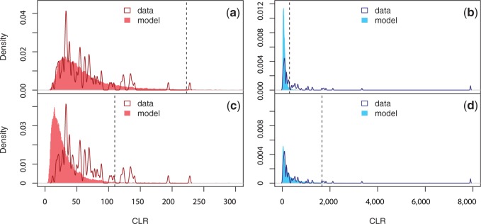
Distribution of maximum CLR values in 1-Mb windows. Simulations based on the standard neutral model (constant population size) for southern Sweden (a) and northern Sweden (b). Simulations based on the secondaryContact6 model for southern Sweden (c) and northern Sweden (d). The dashed line indicates the 99% statistical cutoff (223, 303, 110, and 1,667 in a, b, c, and d, respectively).
Table 3.
Comparison of Statistics Derived from the Data and Three Models.
| Statistics | Dataa | secondary- Contact6 | splitMig5 | splitMig- Bottleneck8 |
|---|---|---|---|---|
| ρS/ρNb | 8.3 | 7.9 | 9.2 | 8.5 |
| S/Nc | 1.65 | 1.68 | 1.76 | 1.68 |
| FSTc | 0.17 | 0.17 | 0.16 | 0.16 |
| Tajima’s D Sc | −0.52 | −0.48 | −0.41 | −0.40 |
| Tajima’s D Nc | 0.10 | 0.26 | 0.29 | 0.20 |
| CLRd N | 174 | 148 | 121 | 172 |
| CLRd S | 49 | 23 | 16 | 19 |
aFor synonymous sites.
bMedian of 1-Mb windows.
cFrom jSFS.
dMedian of maximal CLR scores per 1-Mb window.
The tail of the distribution in northern Sweden is longer than expected under the standard neutral model—in other words, the standard neutral model is not conservative. In contrast, the southern Swedish CLR distribution is narrower, which makes critical CLR values based on the standard neutral model overconservative. Using our secondary contact model to determine CLR cutoffs, we are left with six significant loci in northern Sweden and ten in southern Sweden. The strongest signal in both populations remains the global sweep on chromosome 1. However, of the 22 signals reported in northern Sweden by Long et al. (2013), only three local and one global signal remain significant. Although the ranking of regions according to CLR values shifted after subsampling (supplementary fig. S4, Supplementary Material online), the main reason for the loss of significant regions is the demography-corrected significance cutoff for the North. In fact, subsampling strengthened the sweep signals, that is, the CLR values in the tails became higher. The three regions that remained significant in northern Sweden are located on chromosome 5 and two of them show a significant enrichment for single nucleotide polymorphisms (SNPs) that are correlated with consecutive number of cold days (Hancock et al. 2011). In contrast, nine new significant regions have been identified in southern Sweden and only one shows such an enrichment of SNPs with correlations to environmental variables. (table 4).
Table 4.
Characterization of the Significant Sweep Regions.
| Chr | Position ×103a | CLR | FSTb | α | Population | Significant Enrichment of Gene Environment Correlations (P < 0.05) | Mean Experimental- Recombination Rate |
|---|---|---|---|---|---|---|---|
| 1 | 11,417 | 133 | 0.22 | 47.22e-06 | South | — | 0.029 |
| 1 | 12,855 | 194 | 0.31 | 33.31e-06 | South | — | 0.037 |
| 1 | 19,020 | 1,845 | 0.45 | 2.02e-06 | North | — | 0.016 |
| 6,217(N) | 0.62e-06 (N) | North and | |||||
| 1 | 20,009c | 127(S) | 0.68 | 33.08e-06 (S) | South | — | 0.014 |
| 1 | 24,521 | 141 | 0.16 | 40.81e-06 | South | — | 0.027 |
| Consecutive cold days, | |||||||
| 2 | 13,549 | 135 | 0.14 | 23.22e-06 | South | Relative humidity | 0.024 |
| 3 | 14,961 | 123 | 0.15 | 31.76e-06 | South | — | 0.009 |
| 4 | 5,552 | 228 | 0.11 | 36.92e-06 | South | — | 0.041 |
| 4 | 6,637 | 1,748 | 0.25 | 3.21e-06 | North | — | 0.045 |
| 4 | 9,374 | 120 | 0.16 | 34.85e-06 | South | — | 0.026 |
| Aridity, length of growing season, | |||||||
| Max. precipitation, min. precipitation, | |||||||
| 5 | 2,228 | 1,658 | 0.55 | 1.62e-06 | North | Relative humidity | 0.017 |
| 5 | 5,780 | 122 | 0.32 | 60.59e-06 | South | — | 0.014 |
| 5 | 6,748 | 2,118 | 0.54 | 1.69e-06 | North | Consecutive cold days, daylength | 0.025 |
| 5 | 19,815 | 135 | 0.68 | 51.30e-06 | South | — | 0.015 |
| Consecutive cold days, daylength, | |||||||
| 5 | 26,166 | 1,829 | 0.37 | 1.91e-06 | North | Max. temperature, min.temperature, PAR | 0.021 |
aPositions of the putative sweep regions are rounded to kb.
bLargest value of 100-kb windows within 1 Mb around the CLR peak.
cContains a transposition which is collapsed to a single bp for calculation of FST and CLR.
Evidence of Local Adaptation in Northern Sweden
The next puzzle from our sweep scan is that we detect only one single sweep common to both populations, with the remaining five and nine sweep loci detected in only one of the populations. If sweeps occurred in both populations, with the same strength of selection, we would have had the power to detect all northern sweeps in the South (table 5). We show that this is not due to lack of power by simulating hard selective sweeps with a selection coefficient of s = 0.01, this creates sweep signals near the detection threshold in northern Sweden (see Materials and Methods). We chose the start time of selection to be 0.05 coalescent time units (, corresponding to 25,000 years), which is approximately the time the advantageous allele needs to reach fixation. Furthermore, in accordance with the population mutation rate, we assume that advantageous mutations are ten times more likely to originate in the South. The fixation probability, on the other hand, does not differ depending on whether mutations originated in southern or northern Sweden (0.021 vs. 0.019), nor does the power to detect a sweep (table 5). The probability of detecting sweeps in southern Sweden originating from either location is close to one (; sweep-origin S/sweep-origin N).
Table 5.
Power and Fixation Probability for Selective Sweeps Assuming the secondaryContact6 Demographic Model.
| s | Start Time of Sweep | Population | Origin of Selected Mutation | Mean CLR North | Power North | Mean CLR South | Power South | Fixation Probability |
|---|---|---|---|---|---|---|---|---|
| 0.0025 | 0.12 | Global | South | 250 | 0 | 210 | 0.54 | 0.004 |
| 0.0025 | 0.12 | Global | North | 460 | 0.01 | 270 | 0.7 | 0.004 |
| 0.0025 | 0.12 | Local south | South | 260 | 0 | 250 | 0.65 | 0.004 |
| 0.0025 | 0.12 | Local south | North | 360 | 0.04 | 150 | 0.34 | 0 |
| 0.0025 | 0.12 | Local north | South | 300 | 0.01 | 30 | 0 | 0.001 |
| 0.0025 | 0.12 | Local north | North | 640 | 0.08 | 25 | 0 | 0.007 |
| 0.01 | 0.05 | Global | South | 400 | 0.02 | 1,100 | 0.99 | 0.021 |
| 0.01 | 0.05 | Global | North | 630 | 0.05 | 900 | 1 | 0.019 |
| 0.01 | 0.05 | Local south | South | 260 | 0 | 1,030 | 0.98 | 0.02 |
| 0.01 | 0.05 | Local south | North | 290 | 0 | 930 | 0.96 | 0.001 |
| 0.01 | 0.05 | Local north | South | 510 | 0.08 | 30 | 0.02 | 0.003 |
| 0.01 | 0.05 | Local north | North | 880 | 0.19 | 30 | 0.02 | 0.025 |
| S:0.0025 N:0.01 | 0.05 | Global | South | 493 | 0.05 | 51 | 0.07 | 0.002 |
| S:0.0025 N:0.01 | 0.05 | Global | North | 746 | 0.09 | 50 | 0.1 | 0.022 |
| S:0.0025 N:0.01 | 0.12 | Global | South | 335 | 0 | 242 | 0.68 | 0.013 |
| S:0.0025 N:0.01 | 0.12 | Global | North | 531 | 0.05 | 269 | 0.69 | 0.014 |
Furthermore, we simulated a scenario of global selection with different average selection strength and local selection. As before, we assume that the same allele is under selection with s = 0.01 in the North, but weaker selection in the South with s = 0.0025. We have chosen a selection coefficient in the South to match the observed CLR values of sweep regions in southern Sweden (table 4). The power of detecting a global, but weaker sweep in southern Sweden is still at 60–70%. Hence, it seems highly unlikely that the five northern sweeps are global, because we should have also seen some of them in the South (fig. 6a).
Fig. 6.
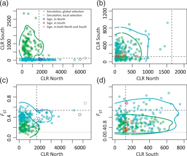
CLR and FST behavior under global and local selection. (a) and (b) are results of a strong sweep (s = 0.01) starting in northern Sweden, (b) and (d) are results of a weak sweep (s = 0.0025) starting in southern Sweden. Green points indicate results under global selection, cyan points indicate results under local selection. The blue and red circles show the CLR and FST values of the significant sweep regions in northern and southern Sweden, respectively. A single sweep region (violet circle) is significant in both northern and southern Sweden. The colored lines are 95% confidence contours. Upper 99% confidence cutoffs for FST and CLR are calculated from 2,400 neutral simulations of 1 Mb sequence and are indicated by the dashed lines. The pointed line indicates the lower 99% cutoff of FST. The msms code for all simulations can be found in supplementary table S5, Supplementary Material online.
One might also speculate that sweeps go undetected in the South because they are more likely to be soft, due to the larger amount of standing variation. We simulated a soft sweep scenario, where the selected mutation has a frequency of 1% or 5% when selection sets in (supplementary table S7, Supplementary Material online). Migration from South to North is so strong that such soft sweeps will also appear weaker in the North. Soft sweeps starting in the South are not only more likely to escape detection in the South, but also in the North and hence we consider this scenario to be less likely than one of strong local selection in the North.
However, for the nine sweeps detected in southern Sweden we cannot determine whether selection was restricted to southern Sweden or simply too weak to be detected in northern Sweden (; sweep-origin S/sweep-origin N) (fig. 6b). If we simulate sweeps under weak selection, the expected distributions of CLR values completely overlap for a scenario of local or global selection. Therefore, we checked whether FST could provide more information to distinguish between the two scenarios and find that we do not gain much power (fig. 6d). Furthermore, only two of the sweeps in southern Sweden have an FST value that is above the 95th percentile of the neutral simulations. The sweep on chromosome 1 that shows a sweep signal in both populations, is one of them. Thus, we cannot say whether the southern Swedish sweeps are global or local.
Besides the little overlap in the selected loci, we also find an unexpected difference in the number of sweep signals: We observe only twice as many sweeps in the South as compared with the North and simulations under global selection with differing selection strength predicts approximately 30 times more sweeps above the significance threshold in the South. Finally, we simulate under a scenario of local selection and differing selection strength: If the selected mutations are beneficial only in one population and selection is stronger in northern (s = 0.01) than in southern Sweden (s = 0.0025), then we find 3–4 times more sweeps in southern Sweden, which is compatible with the observed ratio of approximately 2.
Selection in Northern Sweden Is Stronger and More Prevalent
Due to the demography, sweeps in northern Sweden must be much stronger relative to southern Sweden to produce a significant signal (see section Impact of A. thaliana Demography on SweepFinder CLR Distributions). We also find an at least 4-fold difference in selection strength of the significant sweep regions between South and North (table 4), implying a relatively large mean difference in selection coefficients, with stronger selection in northern Sweden. In the following, we test whether homogeneous selection plus demography can explain the difference in the effective selection strength or whether it indeed differs between North and South.
Simulations with global selection with equal selection strength of s = 0.01 produce CLR values of approximately 1,000, much higher than the highest observed value (CLR = 228). In contrast, similar sweeps in the North will only be detected in a minority of cases (P = 2–19%) and appear weaker (400 < CLR < 880, table 5). Given that the power to detect sweeps is larger in southern Sweden, the number of sweeps is expected to be larger than in northern Sweden and we see approximately twice as many. If the selection strength in southern and in northern Sweden was about s = 0.01 (the detection threshold for northern Sweden), we would expect to see approximately 50 times more sweeps in southern Sweden irrespective of whether selection is global or local. This strongly contradicts the empirical results of only twice the number of significant sweeps in southern Sweden, and argues for differences in the selection coefficient.
Interestingly, also the selection strength of the chromosome 1 sweep was estimated to be smaller in southern Sweden as compared with northern Sweden, suggesting that the weak selection in southern Sweden is not a property of a particular locus, but rather a general phenomenon.
Explaining Weaker Selection
There are two potential explanations for stronger local selection in northern Sweden: Either selection pressures are generally stronger in a peripheral population, or local environments in southern Sweden may conceivably be more heterogeneous than in northern Sweden. In the later case, we would underestimate the true selection strength in the South by averaging over hidden substructure. If selection acts within a subpopulation and is maybe even disadvantageous in neighboring populations, the selected haplotype would quickly reach an intermediate frequency and remain at that frequency for some time. This would result in a molecular footprint similar to the one produced by incomplete sweeps, which can be detected with the iHS statistic (Voight et al. 2006). Indeed, if we compare the iHS statistic of the data to the secondaryContact6 model, the iHS distribution for southern Sweden is wider than compared with simulations from our model (P = 4.0 × 10⁻⁷, supplementary fig. S11, Supplementary Material online).
Furthermore, we compare the ratio of nonsynonymous (PN) over synonymous polymorphisms (PS) in southern Sweden with the one in northern Sweden. Under a heterogeneous scenario we would expect northern Sweden to have a lower ratio than southern Sweden. In contrast, if selection is homogeneous within both demes, that is it only differs between them, we would expect the opposite pattern. This is because PN in a homogeneous population is mostly due to slightly deleterious variants. These should be less frequent in the South because selection is more efficient in a larger population. Using the weighted average over all genes yields that in southern Sweden is 1.05 times larger than in northern Sweden. If we permute the population identifiers, we get odds-ratios that vary between 0.981 and 1.020, that is, significantly smaller than the observed 1.05. In other words, if we take northern Sweden as our expectation, we have a 5% excess of nonsynonymous polymorphisms in southern Sweden, supporting the hypothesis that selection is heterogeneous within southern Sweden.
Discussion
Arabidopsis thaliana of northern Sweden has long been recognized as an outlier to the otherwise continuous isolation by distance of this weedy plant across Europe. The contrast to its nearest neighbors in southern Sweden, which fall right within the European continuum, provides a unique opportunity to investigate local selection. Our analysis shows that a careful estimate of the demographic history is indispensable for any bottom-up analysis of adaptation in A. thaliana.
Arabidopsis thaliana Demography
For Swedish A. thaliana populations, we obtain a secondary contact model as our most likely scenario. In particular, two robust predictions concerning the demography emerge from our results. First, we estimate a surprisingly ancient split time between northern and southern Sweden, about 153 kya (124–182 kya), which is older than a previous estimate of approximately 14 kya close to the beginning of our current warm period (François et al. 2008), but more similar to estimates for the split time among Spanish and Italian A. thaliana of 83 kya (Mathew et al. 2013). This old split time does not depend on data preprocessing (such as subsampling) and it is not specific to our best-fitting model, but robust across various model topologies. The lower bound of the estimated split time of 124 kya coincides with the Eemian interglacial period, which is the first interglacial period where global temperatures reached levels similar to today’s. After the split, the ancestors of the northern and southern Swedish populations either went through a bottleneck or were completely separated for at least 100,000 years before migration resumed. A secondary contact model seems plausible, if the ancestors of northern and southern Swedish plants outlasted the cold periods in different refugia or pockets (Taberlet et al. 1998; Tzedakis et al. 2013).
The second robust result of our demographic inference is that we find twice as many migrants each generation moving from North to South than vice versa forward in time. There are four possible scenarios to explain this: 1) Plants from the very South of southern Sweden are unlikely to migrate directly into the North. If no more than approximately 5% of the southern Swedish seeds could migrate directly, this would explain the observed asymmetry. The asymmetric migration rate could thus also be a result of ghost demes, that is, unsampled populations in-between the North and the South (Beerli 2004). Similarly, this effect will be exacerbated by European immigrants that are expected to be numerous in the very South of Sweden. 2) One would also expect asymmetric migration rates if a previously established population in southern Sweden was replaced by better adapted plants from central Europe after the last glaciation. Indeed, a model of an admixture pulse from central Europe into the South fits well (splitAdmixture9, table 1 and supplementary fig. S10, Supplementary Material online). Note that migration was forced to be symmetric for this model, that is, proportional to the population sizes. 3) If we believe that the northern Swedish population was adapted to its environment and selection in the North is on average stronger than in the South,then migrants from southern Sweden are expected to have a lower fitness in the North, thus reducing the effective migration rate from South to North. In the following, we will discuss further evidence for such a local selection scenario.
Evidence for Local Selection
Signatures of demography and selection are inherently difficult to disentangle. SweepFinder attempts to achieve this by using the background site frequency spectrum to correct fordemography and critical values are obtained by simulating under the standard neutral model. This approach is supposedly robust for many of the originally tested scenarios (Nielsen et al. 2005). Long et al. (2013) describe very different selective sweep patterns in northern and southern Swedish A. thaliana, with SweepFinders CLR statistic showing strong signals for recent selection only in the northern Swedish population.
If we simulate under our secondaryContact6 model, the entire CLR distribution for northern Sweden is shifted to the right (fig. 5 and supplementary fig. S9, Supplementary Material online). In contrast, the CLR distribution for southern Sweden is shifted to the left. Thus significance cutoffs based on the standard neutral model would be too conservative in southern Sweden and too liberal in northern Sweden. The reason for sweep-like patterns in the North, as seen in the right shift of the CLR distribution, might be the relatively large migration rate from southern Sweden to northern Sweden after a long separation of the two populations. This leads to marginal coalescent trees that are characterized by migrant lineages originating from southern Sweden. The sweep like regions in northern Sweden are characterized by fewer migrant lineages than elsewhere in the genome, and low diversity among the nonmigrating lineages due to the small effective population size of the northern population, mimicking the coalescent tree expected after a selective sweep (Jensen et al. 2005). Thus, secondary contact demographies have the potential to confound the SweepFinder statistic, even leading to such curious effects as that, at the same time, the demography of Swedish A. thaliana creates opposite detection biases for northern and southern Sweden if not explicitly accounted for. We expect that similar effects will be observed for other species that follow a secondary contact model, that is, most sessile species that as A. thaliana had to retreat to refugia during glaciation in Europe.
Once we account explicitly for the demographic history of these populations, we do find evidence for true positives among the selective sweep signals in northern Sweden: Three of the Long et al. (2013) sweeps remain significant with the demography-informed cutoffs. Moreover, we also find nine sweep signals in southern Sweden that before were masked by demography. However, there is still surprisingly little overlap between the sweeps in the North and in the South. We assessed whether this pattern could occur by chance under global selection, that is one variant would experience positive selection in both North and South. Simulating scenarios of global selection under the estimated demography, we predict a ratio of significant sweep signals in southern Sweden compared with northern Sweden of 30–50×, which is in contrasts to the actual value of approximately 2. Based on this power analysis, and the fact that global sweeps detected in the North would not go unnoticed in the South, we suggest that adaptation is predominantly local in A. thaliana.
Differing Selection Strength
Moreover, we find that the effective selection strength in the North is at least four times higher than in the South. There are two possible explanations for the stronger sweep signals in northern Sweden: 1) More recent selection in northern Sweden, perhaps due to a recent colonization of an extreme environment. In this case, selection is still local, but the beneficial mutation rate of strongly selected mutations is higher in the North because the population is further from its optimal state (Orr 2005). 2) Selection coefficients appear smaller in the South, due to more population structure and a more heterogeneous environment (fields, cities, beaches, pasture in the South vs. just mountain slopes in the North). Plausibly, the heterogeneity within southern Sweden could also be due to patches of European immigrants. Under these scenarios, selection could still be strong in southern Sweden, but only act within small subpopulations (e.g., A. thaliana on pastures), but we estimate an averaged selection coefficient over all subpopulations.
We find two lines of support for the second scenario: First, only southern Sweden shows an increased propensity for frequent long haplotypes, that can be indicative of partial sweeps that would be expected if selection was confined to only part of the assayed population. Second, local selection is predicted to capture nonsynonymous mutations for environmentally important genes when the environment is heterogeneous and positively selected mutations are not beneficial in all environments (Lee and Mitchell-Olds 2012), yielding a higher ratio of nonsynonymous to synonymous polymorphisms in southern Sweden than in northern Sweden. If these nonsynonymous polymorphisms are only slightly deleterious and neutral, we would expect the opposite due to the larger populations size of the southern population. Instead, the excess of nonsynonymous polymorphisms probably represents locally adapted variants in the heterogeneous southern Swedish population.
Concluding Remarks
Previous selection scans in genome-wide data of A. thaliana did not find much evidence for species-wide selective sweeps (Clark et al. 2007), and the estimated rate of adaptive evolution is rather small for plants in general (Gossmann et al. 2010). However, if selection is acting predominantly on a local scale, both patterns are expected and do not point to low levels of adaptation, but rather to local adaptation. Our results point to two caveats when searching for genomic footprints of selection in structured populations: First, the demographic past has a strong impact on the interpretation of sweep-like genomic variation. Second, environmental and ecological structure hampers the ability of beneficial mutations to sweep through the population quickly and leave a strong sweep signal. For species with little migration, a sweep screen will be more successful in populations with little environmental and demographic substructure. By carefully taking demographic aspects into account, we show that evidence for selective sweeps can be found also in structured populations. Furthermore, we show that the strong sweep signals in northern Sweden are restricted to northern Sweden alone, and in southern Sweden selection is even more local: The lack of strong sweep signals in southern Sweden is most likely a consequence of a heterogeneous environment.
Materials and Methods
Data Processing
We used a data set of 180 sequenced A. thaliana lines from Sweden (Long et al. 2013). The reads in bam file format (Li et al. 2009) can be found in the NCBI short read archive under the project id SRP01289. The reads were filtered for nonuniquely mapped reads and reads with mapping quality smaller than 30. We also filtered for positions with coverage smaller than 4 or larger than 200 within each line, and excluded read positions with base quality smaller than 20. If positions show evidence for heterozygosity (two different bases are supported with more than three reads each) those positions where also excluded.
For deriving the jSFS that was used for demographic inference, we considered only sites with genotype information in each line and excluded sites that are invariant or show more than two alleles.
Classification of SNPs into synonymous, nonsynonymous, intergenic, and intronic was done with the software snpEff (Cingolani et al. 2012) using the A. thaliana genome annotation TAIR9 version April 10, 2012, accessed on May 28, 2012. When several transcripts cover a site, it is possible that the same SNP is classified into several categories. In such cases, a SNP is only classified as synonymous if no alternative classification is into the nonsynonymous class. It turns out that from the four classes (syn., nonsyn., intron, intergenic), synonymous SNPs have the least skewed SFS, in accordance with (Kim et al. 2007), suggesting that synonymous SNPs are the most neutral class (supplementary fig. S1, Supplementary Material online).
For converting estimated coalescent times into generations, it is necessary to know the sequence length that is represented by the SNPs that we chose for demographic inference. It was calculated by counting the total number of polymorphic and invariant sites that are successfully genotyped in all 180 lines and that can also be polarized (i.e., A. lyrata allele is known and matches one of the A. thaliana alleles): L = 27.5 Mb. Of those sites, 2.55 Mb are 4-fold degenerate.
The calculation of the sweep statistics (SweepFinder, FST) was based on all available SNPs. SweepFinder can cope with both missing data and incomplete ancestral state information (mix of polarized and unpolarized SNPs). Although the ancestral state might be misinferred, we chose to polarize SNPs whenever possible. Because SweepFinder is based on the background site frequency spectrum as the null model, the same rate of wrongly inferred ancestral states in both the background and the specific site that is tested should not amount in false positive sweep signals. We also run SweepFinder on unpolarized SNPs, and both estimates of the statistic show a high correlation. We did not consider sweep signals in regions close to the centromeres due to low data quality in this regions, using the same cutoffs as in (Cao et al. 2011; Long et al. 2013).
PCA was done in R version 2.13.2, using the function svd(). Only bialleleic SNPs with full sample size were considered. Principal components were extracted from a singular value decomposition of the normalized data matrix (McVean 2009).
The sweep statistic iHS (Voight et al. 2006) was calculated in R with the package rehh (Gautier and Vitalis 2012) from bialleleic, full sample-size SNPs that could be polarized into ancestral and derived. To test for deviations of the iHS distribution from normality, the Anderson–Darling normality test was used (R package nortest). SNPs were LD pruned using a cutoff of r2 < 0.1 in windows of 200 SNPs.
Demographic Inference with
The input data of consists of a jSFS of only biallelic, synonymous SNPs that have full sample size. Of all polymorphic sites of our sample, 0.7% have 3 nt, 0.005% have 4 nt. Those polymorphisms were removed from further analysis. The jSFS was calculated from 177 plants (128 from southern Sweden, 49 from northern Sweden; three plants were excluded, see Long et al. [2013]). To reduce the influence of sequencing errors, we excluded singletons from the fitting process. To check how different filtering choices (both on the level of individuals and on the level of SNPs) impact parameter estimation, we refitted the secondaryContact6 model to data sets with varying degrees of filtering (see supplementary table S4, Supplementary Material online). Overall, the effect of the filtering steps was relatively small, and confidence intervals for parameters are overlapping. Specifically, they do not change our conclusions regarding the estimated split time and the secondary contact time.
Arabidopsis lyrata is a relatively diverged outgroup and especially the many genomic rearrangements make good alignments and thus the inference of the ancestral state for our sample difficult. Furthermore, the branch to A. lyrata is long enough, so that recurrent mutations are nonnegligible. This in turn might lead to biases when estimating population genetic parameters (Mathew et al. 2013). To avoid this, we based our inference on the folded jSFS.
In total, we tried to fit 14 different models to the two-dimensional site frequency spectrum of the data (see fig. 2 and table 1) using (version 1.6.2; Gutenkunst et al. 2009). To find the globally optimal solution in the parameter space, we repeat each estimation attempt 200 times from randomly chosen initial parameters uniformly sampled in a predefined range of log transformed parameters (supplementary table S1, Supplementary Material online). We required that the parameter combination with the highest likelihood be found at least three times out of the 200 attempts, for all models. Otherwise, additional estimation attempts were run. From the available optimization methods to maximize the likelihood, we chose the simplex algorithm. It turned out to converge faster to the optimal solution than derivative-based alternatives (data not shown). To statistically compare two models, we simulated 100 replicates of genome-wide data from the null model and used to fit parameters for both the null and the alternative model. The simulations were done with msms (Ewing and Hermisson 2010), and the subsequent parameter fitting with was done similar as for the actual data. The corresponding likelihoods for the 100 replicates and the two models where then used to arrive at a null distribution for a likelihood ratio test: We compare a null model to an alternative model by running simulations of data sets based on the null model, calculate the log likelihood ratio for the alternative model relative to the null model (calculated by the log likelihood for the null model minus the log likelihood for the alternative model), and calculate the P value as the fraction of iterations with a likelihood ratio smaller than that for the data.
Using the jSFS, calculates an ancestral θ (, where L is sequence length the jSFS was derived from) that can be used to calculate the ancestral population size given a mutation rate and L. This ancestral population size can then be used to transform time estimates from (in units of ) into actual generations. The L that is used for calculating Ne must reflect the fact that SNPs have been filtered for being synonymous, therefore it is a statistical value that depends on a certain mutational model. However, to calculate effective population size independently of a mutational model, we calculated the jSFS only from 4-fold degenerate sites and estimated Ne from those sites using the respective sequence length of 2.55 Mb.
Coalescent Simulations for Calculating Specificity and Sensitivity of SweepFinder
All simulations were done with the coalescent simulator msms (version 3.2rc, Build:131, see Ewing and Hermisson [2010]), based on the estimated model and parameters from . A sequence length of 1 Mb was simulated with 100 replications for each parameter combination (time of introduction of beneficial mutation, deme of introduction, selection regime—local versus global, selection strength). For the neutral model, 5,000 replications were simulated to calculate a statistical cutoff, allowing for a false positive rate of 1% and therefore for expected 1.2 false positive signals for a genome of size 120 Mb. The window size of 1 Mb was chosen for having good power to detect a selective sweep with selection strength of 0.01 using SweepFinder: Given these parameters, diversity returns to the background level within the window. A single selected mutation (i.e., with a frequency of 1/2/Ne) was placed in the middle of the simulated sequence, and the selected mutation was conditioned on not getting lost during the simulation. The variation in estimated recombination in A. thaliana is relatively large, varying from 0 to 30 cM/Mb along the genome (Giraut et al. 2011). In the simulations, we set recombination rate in A. thaliana to a value of 2.5 cM/Mb, which together with the ancestral population size of 124,000 results in an effective population recombination rate ρ of about 200 (2Ner) per 1 Mb, assuming an inbreeding rate of 97% (Platt et al. 2010). We checked whether this amount of recombination leads to similar LD levels as in the data by estimating the effective recombination rate ρ for both model and data, in southern and northern Sweden separately (fig. 3). ρ was estimated in 1-Mb windows by filtering SNPs for allele frequency of at least 5% and fitting a curve according to (Hill and Weir 1988) to the plot of r2 versus distance in bp. The single parameter of this curve is ρ and is estimated by a nonlinear least squares approach in R.
We simulate selective sweeps both under a model of global selection and under models of local selection. In case of global selection, the introduced beneficial mutation is positively selected in both northern Sweden and southern Sweden. In case of either local southern or local northern Swedish selection, the introduced mutation is only beneficial in the respective deme and neutral in the other.
We choose two parameter combinations for the simulation of selective sweeps: One that reflects the strong signal strength for the significant sweep regions in northern Sweden (s = 0.01, with a time point of introduction of the beneficial mutation of t = 0.05 coalescent time units in the past) and one that reflects the weaker signal strength of significant sweep regions in southern Sweden (s = 0.0025, t = 0.12). The different introduction times reflect the shorter time to fixation of sweeps with larger selection coefficients and were chosen based on a formula for the expected fixation time: . We also tested a scenario where the same mutation is beneficial in both northern and southern Sweden (global selection), but with a smaller selection coefficient in the South (0.0025 in South, 0.01 in North).
For each simulation, summary statistics (FST, θW, π, and Tajima’s D) were calculated in nonoverlapping windows of 10 kb. FST is calculated according to (Hudson 1993). For the discrimination analysis of local versus global sweeps, the largest FST value for each simulated 1-Mb window was recorded. To calculate statistical cutoffs and power, the software SweepFinder (Nielsen et al. 2005) was run on each 1-Mb window along grid points of 1-kb distance. Further, it was assumed that only 50% of SNPs can be polarized to mirror the fact that only 50% have outgroup information from A. lyrata in the actual data set.
Supplementary Material
Supplementary Material figures S1–S11 and tables S1–S7 are available at Molecular Biology and Evolution online (http://www.mbe.oxfordjournals.org/).
Acknowledgments
The authors thank Andrea Betancourt and the reviewers for comments on the manuscript and Greg Ewing for help with the software msms. This work was supported by the Austrian Science Fund (Vienna Graduate School of Population Genetics, FWF W1225) to C.D.H. and by ERC grant 268962—MAXMAP to M.N.
References
- Ågren J, Oakley CG, McKay JK, Lovell JT, Schemske DW. Genetic mapping of adaptation reveals fitness tradeoffs in Arabidopsis thaliana. Proc Natl Acad Sci U S A. 2013;110(52):21077–21082. doi: 10.1073/pnas.1316773110. [DOI] [PMC free article] [PubMed] [Google Scholar]
- Ågren J, Schemske DW. Reciprocal transplants demonstrate strong adaptive differentiation of the model organism Arabidopsis thaliana in its native range. New Phytol. 2012;194(4):1112–1122. doi: 10.1111/j.1469-8137.2012.04112.x. [DOI] [PubMed] [Google Scholar]
- Atwell S, Huang YS, Vilhjlmsson BJ, Willems G, Horton M, Li Y, Meng D, Platt A, Tarone AM, Hu TT, et al. Genome-wide association study of 107 phenotypes in Arabidopsis thaliana inbred lines. Nature. 2010;465(7298):627–631. doi: 10.1038/nature08800. [DOI] [PMC free article] [PubMed] [Google Scholar]
- Beerli P. Effect of unsampled populations on the estimation of population sizes and migration rates between sampled populations. Mol Ecol. 2004;13(4):827–836. doi: 10.1111/j.1365-294x.2004.02101.x. [DOI] [PubMed] [Google Scholar]
- Boyko AR, Williamson SH, Indap AR, Degenhardt JD, Hernandez RD, Lohmueller KE, Adams MD, Schmidt S, Sninsky JJ, Sunyaev SR, et al. Assessing the evolutionary impact of amino acid mutations in the human genome. PLoS Genet. 2008;4(5):e1000083. doi: 10.1371/journal.pgen.1000083. [DOI] [PMC free article] [PubMed] [Google Scholar]
- Bustamante CD, Nielsen R, Sawyer SA, Olsen KM, Purugganan MD, Hartl DL. The cost of inbreeding in Arabidopsis. Nature. 2002;416(6880):531–534. doi: 10.1038/416531a. [DOI] [PubMed] [Google Scholar]
- Cao J, Schneeberger K, Ossowski S, Gnther T, Bender S, Fitz J, Koenig D, Lanz C, Stegle O, Lippert C, et al. Whole-genome sequencing of multiple Arabidopsis thaliana populations. Nat Genet. 2011;43(10):956–963. doi: 10.1038/ng.911. [DOI] [PubMed] [Google Scholar]
- Cingolani P, Platts A, Wang LL, Coon M, Nguyen T, Wang L, Land SJ, Lu X, Ruden DM. A program for annotating and predicting the effects of single nucleotide polymorphisms, SnpEff: SNPs in the genome of Drosophila melanogaster strain w1118; iso-2; iso-3. Fly. 2012;6(2):80–92. doi: 10.4161/fly.19695. [DOI] [PMC free article] [PubMed] [Google Scholar]
- Clark RM, Schweikert G, Toomajian C, Ossowski S, Zeller G, Shinn P, Warthmann N, Hu TT, Fu G, Hinds DA, et al. Common sequence polymorphisms shaping genetic diversity in Arabidopsis thaliana. Science. 2007;317(5836):338–342. doi: 10.1126/science.1138632. [DOI] [PubMed] [Google Scholar]
- Corre VL, Roux F, Reboud X. DNA polymorphism at the FRIGIDA gene in Arabidopsis thaliana: extensive nonsynonymous variation is consistent with local selection for flowering time. Mol Biol Evol. 2002;19(8):1261–1271. doi: 10.1093/oxfordjournals.molbev.a004187. [DOI] [PubMed] [Google Scholar]
- Ewing G, Hermisson J. MSMS: a coalescent simulation program including recombination, demographic structure and selection at a single locus. Bioinformatics. 2010;26(16):2064–2065. doi: 10.1093/bioinformatics/btq322. [DOI] [PMC free article] [PubMed] [Google Scholar]
- Eyre-Walker A, Keightley PD. Estimating the rate of adaptive molecular evolution in the presence of slightly deleterious mutations and population size change. Mol Biol Evol. 2009;26(9):2097–2108. doi: 10.1093/molbev/msp119. [DOI] [PubMed] [Google Scholar]
- Fournier-Level A, Korte A, Cooper MD, Nordborg M, Schmitt J, Wilczek AM. A map of local adaptation in Arabidopsis thaliana. Science. 2011;334(6052):86–89. doi: 10.1126/science.1209271. [DOI] [PubMed] [Google Scholar]
- François O, Blum MGB, Jakobsson M, Rosenberg NA. Demographic history of European populations of Arabidopsis thaliana. PLoS Genet. 2008;4(5):e1000075. doi: 10.1371/journal.pgen.1000075. [DOI] [PMC free article] [PubMed] [Google Scholar]
- Gaut B. Arabidopsis thaliana as a model for the genetics of local adaptation. Nat Genet. 2012;44(2):115–116. doi: 10.1038/ng.1079. [DOI] [PubMed] [Google Scholar]
- Gautier M, Vitalis R. rehh: an R package to detect footprints of selection in genome-wide SNP data from haplotype structure. Bioinformatics. 2012;28(8):1176–1177. doi: 10.1093/bioinformatics/bts115. [DOI] [PubMed] [Google Scholar]
- Giraut L, Falque M, Drouaud J, Pereira L, Martin OC, Mzard C. Genome-wide crossover distribution in Arabidopsis thaliana meiosis reveals sex-specific patterns along chromosomes. PLoS Genet. 2011;7(11):e1002354. doi: 10.1371/journal.pgen.1002354. [DOI] [PMC free article] [PubMed] [Google Scholar]
- Gossmann TI, Song B-H, Windsor AJ, Mitchell-Olds T, Dixon CJ, Kapralov MV, Filatov DA, Eyre-Walker A. Genome wide analyses reveal little evidence for adaptive evolution in many plant species. Mol Biol Evol. 2010;27(8):1822–1832. doi: 10.1093/molbev/msq079. [DOI] [PMC free article] [PubMed] [Google Scholar]
- Gutenkunst RN, Hernandez RD, Williamson SH, Bustamante CD. Inferring the joint demographic history of multiple populations from multidimensional SNP frequency data. PLoS Genet. 2009;5(10):e1000695. doi: 10.1371/journal.pgen.1000695. [DOI] [PMC free article] [PubMed] [Google Scholar]
- Halligan DL, Oliver F, Eyre-Walker A, Harr B, Keightley PD. Evidence for pervasive adaptive protein evolution in wild mice. PLoS Genet. 2010;6(1):e1000825. doi: 10.1371/journal.pgen.1000825. [DOI] [PMC free article] [PubMed] [Google Scholar]
- Hancock AM, Brachi B, Faure N, Horton MW, Jarymowycz LB, Sperone FG, Toomajian C, Roux F, Bergelson J. Adaptation to climate across the Arabidopsis thaliana genome. Science. 2011;334(6052):83–86. doi: 10.1126/science.1209244. [DOI] [PubMed] [Google Scholar]
- Hill WG, Weir BS. Variances and covariances of squared linkage disequilibria in finite populations. Theor Popul Biol. 1988;33(1):54–78. doi: 10.1016/0040-5809(88)90004-4. [DOI] [PubMed] [Google Scholar]
- Horton MW, Hancock AM, Huang YS, Toomajian C, Atwell S, Auton A, Muliyati NW, Platt A, Sperone FG, Vilhjlmsson BJ, et al. Genome-wide patterns of genetic variation in worldwide Arabidopsis thaliana accessions from the RegMap panel. Nat Genet. 2012;44(2):212–216. doi: 10.1038/ng.1042. [DOI] [PMC free article] [PubMed] [Google Scholar]
- Hudson RR. Levels of DNA polymorphism and divergence yield important insights into evolutionary processes. Proc Natl Acad Sci U S A. 1993;90(16):7425–7426. doi: 10.1073/pnas.90.16.7425. [DOI] [PMC free article] [PubMed] [Google Scholar]
- Jensen JD, Kim Y, DuMont VB, Aquadro CF, Bustamante CD. Distinguishing between selective sweeps and demography using DNA polymorphism data. Genetics. 2005;170(3):1401–1410. doi: 10.1534/genetics.104.038224. [DOI] [PMC free article] [PubMed] [Google Scholar]
- Kim S, Plagnol V, Hu TT, Toomajian C, Clark RM, Ossowski S, Ecker JR, Weigel D, Nordborg M. Recombination and linkage disequilibrium in Arabidopsis thaliana. Nat Genet. 2007;39(9):1151–1155. doi: 10.1038/ng2115. [DOI] [PubMed] [Google Scholar]
- Koornneef M, Alonso-Blanco C, Vreugdenhil D. Naturally occurring genetic variation in Arabidopsis thaliana. Annu Rev Plant Biol. 2004;55(1):141–172. doi: 10.1146/annurev.arplant.55.031903.141605. [DOI] [PubMed] [Google Scholar]
- Lee C-R, Mitchell-Olds T. Environmental adaptation contributes to gene polymorphism across the Arabidopsis thaliana genome. Mol Biol Evol. 2012;29(12):3721–3728. doi: 10.1093/molbev/mss174. [DOI] [PMC free article] [PubMed] [Google Scholar]
- Li H, Handsaker B, Wysoker A, Fennell T, Ruan J, Homer N, Marth G, Abecasis G, Durbin R. The sequence Alignment/Map format and SAMtools. Bioinformatics. 2009;25(16):2078–2079. doi: 10.1093/bioinformatics/btp352. [DOI] [PMC free article] [PubMed] [Google Scholar]
- Long Q, Rabanal FA, Meng D, Huber CD, Farlow A, Platzer A, Zhang Q, Vilhjlmsson BJ, Korte A, Nizhynska V, et al. Massive genomic variation and strong selection in Arabidopsis thaliana lines from Sweden. Nat Genet. 2013;45(8):884–890. doi: 10.1038/ng.2678. [DOI] [PMC free article] [PubMed] [Google Scholar]
- Mathew LA, Staab PR, Rose LE, Metzler D. Why to account for finite sites in population genetic studies and how to do this with Jaatha 2.0. Ecol Evol. 2013;3(11):3647–3662. doi: 10.1002/ece3.722. [DOI] [PMC free article] [PubMed] [Google Scholar]
- McVean G. A genealogical interpretation of principal components analysis. PLoS Genet. 2009;5(10):e1000686. doi: 10.1371/journal.pgen.1000686. [DOI] [PMC free article] [PubMed] [Google Scholar]
- Nielsen R, Williamson S, Kim Y, Hubisz MJ, Clark AG, Bustamante C. Genomic scans for selective sweeps using SNP data. Genome Res. 2005;15(11):1566–1575. doi: 10.1101/gr.4252305. [DOI] [PMC free article] [PubMed] [Google Scholar]
- Nordborg M, Donnelly P. The coalescent process with selfing. Genetics. 1997;146(3):1185–1195. doi: 10.1093/genetics/146.3.1185. [DOI] [PMC free article] [PubMed] [Google Scholar]
- Nordborg M, Hu TT, Ishino Y, Jhaveri J, Toomajian C, Zheng H, Bakker E, Calabrese P, Gladstone J, Goyal R, et al. The pattern of polymorphism in Arabidopsis thaliana. PLoS Biol. 2005;3(7):e196. doi: 10.1371/journal.pbio.0030196. [DOI] [PMC free article] [PubMed] [Google Scholar]
- Orr HA. The genetic theory of adaptation: a brief history. Nat Rev Genet. 2005;6(2):119–127. doi: 10.1038/nrg1523. [DOI] [PubMed] [Google Scholar]
- Ossowski S, Schneeberger K, Lucas-Lled JI, Warthmann N, Clark RM, Shaw RG, Weigel D, Lynch M. The rate and molecular spectrum of spontaneous mutations in Arabidopsis thaliana. Science. 2010;327(5961):92–94. doi: 10.1126/science.1180677. [DOI] [PMC free article] [PubMed] [Google Scholar]
- Pavlidis P, Hutter S, Stephan W. A population genomic approach to map recent positive selection in model species. Mol Ecol. 2008;17(16):3585–3598. doi: 10.1111/j.1365-294X.2008.03852.x. [DOI] [PubMed] [Google Scholar]
- Platt A, Horton M, Huang YS, Li Y, Anastasio AE, Mulyati NW, Ågren J, Bossdorf O, Byers D, Donohue K, et al. The scale of population structure in Arabidopsis thaliana. PLoS Genet. 2010;6(2):e1000843. doi: 10.1371/journal.pgen.1000843. [DOI] [PMC free article] [PubMed] [Google Scholar]
- Rutter MT, Fenster CB. Testing for adaptation to climate in Arabidopsis thaliana: a calibrated common garden approach. Ann Bot. 2007;99(3):529–536. doi: 10.1093/aob/mcl282. [DOI] [PMC free article] [PubMed] [Google Scholar]
- Sattath S, Elyashiv E, Kolodny O, Rinott Y, Sella G. Pervasive adaptive protein evolution apparent in diversity patterns around amino acid substitutions in Drosophila simulans. PLoS Genet. 2011;7(2):e1001302. doi: 10.1371/journal.pgen.1001302. [DOI] [PMC free article] [PubMed] [Google Scholar]
- Slatkin M. Seeing ghosts: the effect of unsampled populations on migration rates estimated for sampled populations. Mol Ecol. 2005;14(1):67–73. doi: 10.1111/j.1365-294X.2004.02393.x. [DOI] [PubMed] [Google Scholar]
- Slotte T, Bataillon T, Hansen TT, Onge KS, Wright SI, Schierup MH. Genomic determinants of protein evolution and polymorphism in Arabidopsis. Genome Biol Evol. 2011;3(9):1210–1219. doi: 10.1093/gbe/evr094. [DOI] [PMC free article] [PubMed] [Google Scholar]
- Slotte T, Foxe JP, Hazzouri KM, Wright SI. Genome-wide evidence for efficient positive and purifying selection in Capsella grandiflora, a plant species with a large effective population size. Mol Biol Evol. 2010;27(8):1813–1821. doi: 10.1093/molbev/msq062. [DOI] [PubMed] [Google Scholar]
- Taberlet P, Fumagalli L, Wust-Saucy AG, Cosson JF. Comparative phylogeography and postglacial colonization routes in Europe. Mol Ecol. 1998;7(4):453–464. doi: 10.1046/j.1365-294x.1998.00289.x. [DOI] [PubMed] [Google Scholar]
- Tzedakis PC, Emerson BC, Hewitt GM. Cryptic or mystic? Glacial tree refugia in northern Europe. Trends Ecol Evol. 2013;28(12):696–704. doi: 10.1016/j.tree.2013.09.001. [DOI] [PubMed] [Google Scholar]
- Voight BF, Kudaravalli S, Wen X, Pritchard JK. A map of recent positive selection in the human genome. PLoS Biol. 2006;4(3):e72. doi: 10.1371/journal.pbio.0040072. [DOI] [PMC free article] [PubMed] [Google Scholar]
- Wright SI, Andolfatto P. The impact of natural selection on the genome: emerging patterns in Drosophila and Arabidopsis. Annu Rev Ecol Evol Syst. 2008;39(1):193–213. [Google Scholar]
Associated Data
This section collects any data citations, data availability statements, or supplementary materials included in this article.