Quantifying uncertainties in the microvascular transport of nanoparticles

Abstract

The character of nanoparticle dispersion in the microvasculature is a driving factor in nanoparticle-based therapeutics and bio-sensing. It is difficult, with current experimental and engineering capability, to understand dispersion of nanoparticles because their vascular system is more complex than mouse models and because nanoparticle dispersion is so sensitive to in vivo environments. Furthermore, uncertainty can not be ignored due to the high variation of location-specific vessel characteristics as well as variation across patients. In this paper, a computational method that considers uncertainty is developed to predict nanoparticle dispersion and transport characteristics in the microvasculature with a three step process. First, a computer simulation method is developed to predict blood flow and the dispersion of nanoparticles in the microvessels. Second, experiments for nanoparticle dispersion coefficients are combined with results from the computer model to suggest the true values of its unknown and unmeasurable parameters – red blood cell deformability and red blood cell interaction – using the Bayesian statistical framework. Third, quantitative predictions for nanoparticle tranpsort in the tumor microvasculature are made that consider uncertainty in the vessel diameter, flow velocity, and hematocrit. Our results show that nanoparticle transport is highly sensitive to the microvasculature.

1 Introduction

Nanoparticle (NP) transport in the microvasculature (Ferrari 2005; Duncan 2006; Peer et al. 2007) has been of interest in new diagnosis and treatment of diseases. However, after synthesizing the NPs for systemic injection, experiments that aim to see NP dispersion in the microvasculature are limited to a small number of mouse models (Decuzzi et al. 2010; Chauhan et al. 2012; Cabral et al. 2011; van de Ven et al. 2012). Recently, experiments and simulations have been used to characterize the NP transport. Chauhan et al. (2012) studied the NP size effect on mammary tumors by using in vivo experiments and mathematical models. Sinek et al. (2009) predicted the pharmocokinetics and effect of drugs in a tumor environment by simulation. Also, at the nanoarticle level, blood flow simulations (Lee et al. 2013) were performed to capture NP movement in a microvessel model including blood plasma, red blood cell (RBC), and NP drug carriers. In addition, several studies were performed to understand NP dispersion in the microvessel (Namdee et al. 2013; Tan et al. 2012; Saadatmand et al. 2011).

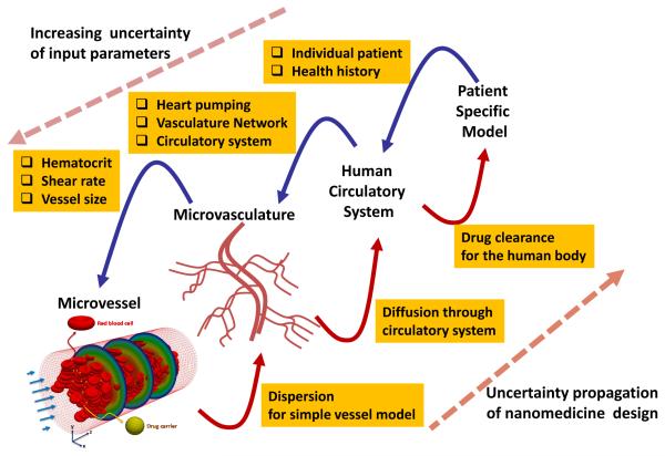
Though that computer simulations and in vivo experiments gave useful results uncovering the mechanisms of NP motion in a confined microvascular system with specific size and flow characteristics, the results were difficult to extrapolate to other portions of the microvasculature due to the wide variation of these attributes (vessel size, flow, contents). Concordantly, for directly delivering NPs to the deseasd area, it is required to characterize the microvasculature of the targeted area in the body. So, the inclusion of microvascular information into the computational model, heretofore ignored in flow predictions, is critical to improving predictions of NP movement and drug carrier efficiency in the blood stream. Furthermore, the escape of NPs from the vessel by diffusion through the vessel wall should be considered. Extending the model to the tissue and target cells of therapeutic efforts requires the consideration of more important factors such as the enhanced permeability and retention (EPR) effect, specific/non-specific binding, and cellular uptake. A general model that can capture the journey of NPs from blood flow to a patient’s cell is more complex as shown in Fig. 1.

Fig. 1.

Uncertainty of NP transport in the multiscale vascular system

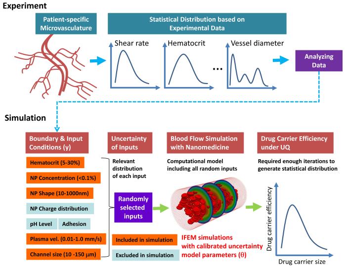
For more predictive design of NPs, we suggest a computational method that considers uncertainty. The ultimate goal of nanomedicine for cancer therapeutics is to ensure as many drug-carrying NPs as possible reaching the cancerous region in the human body after their injection of NPs into the blood stream. Here, the simulation parameters for blood flow are calibrated by a Bayesian updating algorithm and subsequently used to perform computational prediction of drug carrier efficiency in the microvasculature. However, such a simulation model is not enough to describe the entire microvasculature which, depending on location, has different geometric features and flow conditions. As shown in Fig. 2, we propose a procedure of computational drug design that combines experiments, simulations of drug carrier dispersion, and statistical models of input and output uncertainty. Because simulating the entire microvasculature and the RBCs/NPs contained within is computationally intractable, real variations at the microvasculature level can be replaced with random models applied to the inputs of local blood vessel simulations. Experimental data collected at different points in the microvasculature for shear rates, hematocrit, and vessel diameter, for instance, produce the random models for local vessel models. With random input statistical distributions defined, uncertainty is propagated through the high fidelity fluid-structure interaction model of the blood vessel, which contains both RBCs and NPs and their interactions, to outputs that measure drug carrier efficiency such as dispersion coefficients or NP ensemble drift velocity.

Fig. 2.

Uncertainty quantification of NPs in the microvasculature using experiement and simulation

In this paper, to realize the concept of nanomedicine design, we combine physics-based flow simulations with uncertainty quantification (UQ) techniques for the prediction of NP transport in the microvasculature. The immersed finite element method (IFEM) (Zhang et al. 2004; Liu et al. 2006; Lee et al. 2008; Liu et al. 2007a,b; Kopacz et al. 2012; Kopacz and Liu 2013) serves as the physics-based, high fidelity model of the blood vessel. Since some parameters in this model are unknown and unmeasurable, their true values are elucidated with a Bayesian updating method (Kennedy and O’Hagan 2001; Bayarri et al. 2007). The updated physics-based model serves as the conduit through which uncertainty is propagated using a moment-matching stochastic collocation method (Lee and Chen 2009). The uncertainty quantification algorithms perform two tasks: (1) updating IFEM model and (2) propagating microvasculature uncertainty through the updated model to make statistical predictions about nanoparticle transport phenomena under the uncertainty in the blood vessel network. To demonstrate the translational possibility, the nanoparticle dispersion is predicted in a tumor microvascular environment which is measured from in vivo image (Kamoun et al. 2010).

2 Materials and Methods

2.1 NP transport simulation in blood flow: IFEM approach

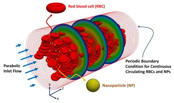
A fluid-solid interaction (FSI) system as shown in Fig. 3 is considered to simulate the entire domain including blood plasma, RBCs, and NPs in a microvessel. A periodic boundary condition for RBCs and NPs is applied that inserts them in the inlet on the left after they escape from the outlet on the right. The IFEM (Zhang et al. 2004; Liu et al. 2006; Lee et al. 2008; Liu et al. 2007a,b; Kopacz et al. 2012; Kopacz and Liu 2013) for simulating both fluid (blood plasma) and solid (RBCs and NPs) is constructed on an Eulerian domain (Ω) which includes fluid and solid domains. The IFEM on Ω is governed by Navier-Stokes equations with FSI force (f^FSI) defined as:

$$\rho f\left(\frac{\partial u}{\partial t}+u\cdot \nabla u\right)+\nabla p-{\mu }_f{\nabla }^{2}u=f_f+f^{FSI},$$ (1)

$$\nabla \cdot u=0,$$ (2)

where ρ_f is the density of the blood plasma, u is the velocity, t is the time, p is the pressure, μ_f is the viscosity of the blood plasma, f_f is the external force acting on the blood plasma, and f^FSI is the FSI force for recognizing the solid objects in the whole domain. The Mooney-Rivlin material model (Liu and Liu 2006) is used for the RBCs to account for hyperelastic deformation. The RBC deformability μ₀ is the initial in-plane membrane shear modulus. It is defined as μ₀ = 0.75G₀h₀ where G₀ is the shear modulus and h₀ is the membrane thickness (Dao et al. 2003). In this computational model, f^FSI contains separate contributions from the molecular interactions of RBC-RBC, RBC-NP, and NP-NP pairs.

Fig. 3.

Computer simulation model for calculating radial dispersion coefficient of NPs. In the microvessel, blood plasma, RBCs, and NPs are simulated by the IFEM computer code.

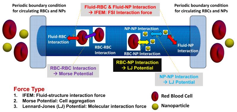
As shown in Fig. 4, various interactions occur in the microvessel among blood plasma, RBCs, and NPs. In this computational model, we consider RBC-RBC, RBC-NP, and NP-NP interactions. The RBC-RBC interaction is described by a Morse-type potential (Zhang et al. 2008; Liu and Liu 2006) given as:

$${\Phi }_M\left(r\right)=D_e\left[e^{2\beta (r_0-r)}-2e^{\beta (r_0-r)}\right],$$ (3)

where D_e is the Morse potential amplitude, β is the scaling factor, r₀ is the critical length for zero-force, and r is the distance between RBC surface nodes. Also, the interaction forces for RBC-NP and NP-NP are described by a Lennard-Jones potential as

$${\Phi }_{LJ}\left(r\right)=4∊\left[{\left(\frac{r_m}{r}\right)}^{12}-{\left(\frac{r_m}{r}\right)}^6\right],$$ (4)

where ε is the scaling parameter and r_m is the equilibrium length.

Fig. 4.

Schematic of interaction forces in a microvessel

Since we seek computation of NP radial dispersion characteristics (described by vector D), which arise from the solution of the IFEM model, we can write the dispersion characteristics as a function of the IFEM model parameters:

$$D=\mathcal{D}(D_e,\beta ,r_0,{∊}^{RBC-NP},r_m^{RBC-NP},{∊}^{NP-NP},r_m^{NP-NP},{\mu }_0,\dots ).$$ (5)

Two of the above parameters are the RBC deformability (μ₀) and RBC-RBC interaction potential amplitude (D_e), which while required by the model are not easily measured by experimental techniques and thus have uncertain values. This means they may also be used to calibrate the IFEM model to match known experimental results. The general model updating framework is presented in the following section.

For the NP transport simulations and experiments with a number of particles N, a quantity of interest is the radial dispersion coefficient, which is defined mathematically by (Saadatmand et al. 2011)

$$D_R=\frac{1}{N}\sum _{i=1}^N\frac{\langle {\left[r_i\right(t)-r_i(0\left)\right]}^2\rangle }{2t},$$ (6)

where r_i(t) is the distance of the NP from the center of the channel at the time t and r_i(0) is the initial distance. The angled brackets ⟨0⟩ indicate the expectation with respect to time, which is an average of the interior quantity up until time t. t is considered sufficiently long so an equilibrium state is reached. Physically, the dispersion coefficient (units are μm²/s) averages the variance of a particle position from its initial value over all the particles. Thus, a high dispersion coefficient means a large amount of “mixing” occurs of NPs in the blood stream, whereas a small value indicates a low probability that NPs deviate in a perpendicular direction from the vessel centerline. A high dispersion coefficient, therefore, is desirable from a drug delivery standpoint: as NPs are more likely to deviate from their initial positions so are they more likely to diffuse through the vessel wall and penetrate (potentially) damaged cell tissue.

2.2 Bayesian calibration of the model parameters

In this subsection, the approach for combining experimental and computational results to update a computer model that leverages the Bayesian statistical framework is briefly presented. The methodology for combining numerical and physical experiments follows that described by Bayarri et al. (2007), and here we further adopt the modular Bayesian approach as outlined in Kennedy and O’Hagan (2001). This approach recognizes three sources of uncertainty in computational predictions: the unknown values of model parameters (θ), lack of knowledge due to missing physics in the model, and experimental error. Experimental data for a quantity of interest z, here the dispersion coefficient z = D_R, may be written as a superposition of three terms:

$$z^e\left(H\right)=z^m(H,\theta )+\delta \left(H\right)+\epsilon ,$$ (7)

where superscripts e and m indicate experimental and model observations, δ is a discrepancy function accounting for the inadequacy of the model to correctly describe the observations, and ε ~ N(0, σ_e) is the experimental error assumed to be distributed normally with zero mean and constant variance. Here, H is the hematocrit, a variable common to experiments and model, though in general this portion of the formulation may be multidimensional. θ indicate the parameters whose value we aim to update with the Bayesian formalism. Here, θ = [μ₀, D_e] contains the RBC deformability and RBC-RBC interaction potential amplitude.

In this and the ensuing subsection, random variables will be given in uppercase (e.g. V) with a realization in lower case (e.g. v) unless otherwise noted. In the Bayesian calibration process, the model parameters are assumed to be a multivariate random vector Θ with posterior probability distribution function

$$f_{ϴ}(\theta \mid z)=\frac{1}{C}{f}_Z(z\mid \theta )f_{ϴ}\left(\theta \right),$$ (8)

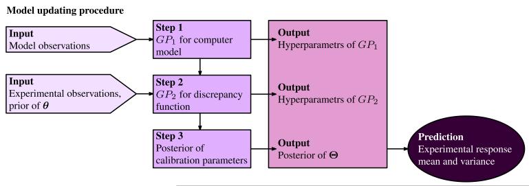
where f_Z(z|θ) is the likelihood distribution, the probability of observing z given a parameter set θ, f_Θ (θ) is a prior distribution on the calibration parameters typically specified by field experts, literature, or low-fidelity simulations, and C is a normalization constant to ensure the posterior integrates to one over its domain. The computation of the posterior distribution involves the following key steps (shown in Fig. 5).

Fig. 5.

Flow diagram explaining the modular Bayesian approach for model updating. GP represents Gaussian Process, θ is the calibration parameters and Θ is the bivariate random vector.

1. Gaussian process modeling for the computer model. A Gaussian process is a spatial random process that can be used to replace any function. It is capable of capturing the trend and roughness of the function by properly setting a few key parameters, which are called hyperparameters of the Gaussian process. In this step the computer model is replaced by a Gaussian process provided the model observations; its hyperparameters are determined by maximum likelihood estimation (MLE) which maximizes the probability of obtaining the current model observations given a possible hyperparameter set. The determination of hyperparameters is conducted with readily available stochastic or gradient-based optimization methods.

2. Gaussian process modeling for the discrepancy function. Another Gaussian process model is fitted to infer the discrepancy function δ(H) by combining the experimental and model observations, the prior distribution of the calibration parameters, and the hyperparameters of the computer model obtained in the previous step. Independence is assumed between z^m(H, θ), δ(H), and ε, and a similar MLE scheme determines the hyperparameters of the Gaussian process for the discrepancy function.

3. Calculating the posterior of the calibration parameters. The value of the likelihood function f_Z(z|θ) is determined by the two Gaussian processes for the computer model and the discrepancy function; the posterior f_Θ(θ|z) of the parameters is subsequently calculated by eq. (8).

After the computation of the posterior distribution, the full prediction of z^e(H) considering both model discrepancy and parameter uncertainty can be determined by its prediction mean and prediction variance:

$$\begin{array}{cc}\hfill \mu \left(z^e\right(H)\mid z)=& {\langle {\langle z^e\left(H\right)\mid z,\theta \rangle }_z\rangle }_{ϴ}\hfill \\ \hfill & ={\int }_{\mathcal{T}}{\langle z^e\left(H\right)\mid z,\theta \rangle }_z{f}_{ϴ}(\theta \mid z)d\theta ,\hfill \end{array}$$ (9)

$${\sigma }^2\left(z^e\right(H)\mid z)={\langle {\sigma }^2\left(z^e\right(H)\mid z,\theta )\rangle }_{ϴ}+{\sigma }^2\left({\langle z^e\left(H\right)\mid z,\theta \rangle }_z\right).$$ (10)

In the above μ(q) and σ²(q) are the mean and variance of the quantity q. The notation ⟨q⟩_V is the expectation (mean) of the quantity q with respect to random variable V. By this notation, σ²(q) = ⟨(q − μ(q))²⟩ by the definition of statistical variance. In eq. (9), T is the support of the random vector of calibration parameters Θ assumed to follow the posterior distribution. In this implementation, the calibration parameters are assumed to follow an independent multivariate normal distribution so that T = ℝ^M, with M the number of calibration parameters.

The prediction mean expression in eq. (9) says that the predicted value of the experimental observation z^e at value H, given the observations z, equals overall expectation of z^e(H), given z and any possible value of θ from its posterior distribution. The prediction variance expression in eq. (10) says that the true value of z^e(H) may vary from the prediction mean because of two variation sources, one being the variation due to different possible values of θ, the other being the variation due to the random quantity z^e itself even when θ is fixed.

3 Results

3.1 Simulation of NP transport in a microvessel

The blood flow and NP dispersion in a microvessel are simulated to compare with experimental data measuring the dispersion coefficient of particles by inserting RBCs (Saadatmand et al. 2011). To model the given experimental conditions, the density and viscosity of the plasma are 1.046 g/cm³ and 3.8 × 10⁻³ Pa-s, respectively. The tube diameter is 50 μm and the flow rate is 0.033 mL/min. The volume fraction of RBCs (hematocrit) is 0-20%, a domain consistent with experimental data used for Bayesian updating. The RBC density is the same as the plasma and its surface is treated as a hyperelastic, the RBC deformability (μ₀) is 6.0 μN/m. The cytoplasm (Park et al. 2011) in the RBCs is described by a fluid with the same density as the outside of the cells and a viscosity of 6.0 × 10⁻³ Pa-s. Recalling Sec. 2.1, the RBC-RBC intracellular interaction (Zhang et al. 2008; Liu and Liu 2006) is estimated by a Morse-type potential with D_e = 1.0 μJ/m², r₀ = 0.49 μm, and β = 3.84μm⁻¹. Also, a total of 90 NPs with diameters of 1 μm are added in the computational microvessel, which serve as the ensemble by which the dispersion coefficient in eq. (6) is calculated. Each NP is described as a rigid body whose density is the same as that of the plasma. The RBC-NP and NP-NP interactions, to numerically avoid overlapping among them, are described by a Lennard-Jones potential with ε = 1.0 × 10⁻¹² J and r_m = 1.0 nm.

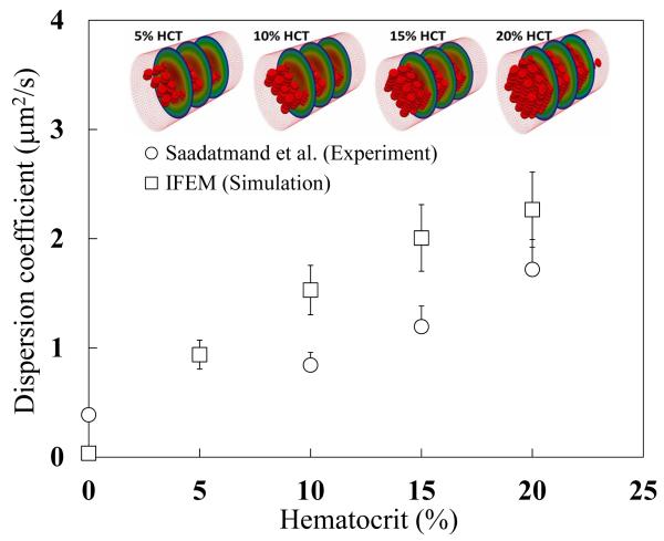
Figure 6 shows the experimental and simulation results at different hematocrit values. Both sets of results show that when hematocrit increases NP dispersion increases as well. The relationship appears to be monotonic from the results, and the value of the dispersion coefficient in experiment and simulation are similar. However, a noticeable gap between the experiments and simulations exists. This error predominantly derives from the absence of a rigorous calibration procedure applied to the parameters of the model shown in eq. (5), which were chosen in the paragraph above based on experience of the authors or values from literature. In next subsection, we will discuss how to update the computational model and calibrate the unknown model parameters by the Bayesian calibration procedure discussed in previous Section.

Fig. 6.

Dispersion coefficient from in vitro experiment Saadatmand et al. (2011) and IFEM simulation. For the prediction of the dispersion coefficient described by eq. (6), the particles with diameters of 1 μm are simulated in a microtube 50 μm in diameter, which is considered as the same condition as the experiment.

3.2 Determination of unknown model parameters

The RBC deformability (μ₀) and RBC-RBC morse potential parameter (D_e) will be used to update the IFEM model where θ₁ = μ₀ and θ₂ = D_e. The parameters are ideal for calibration because the RBC deformation and RBC-RBC interaction are affected to the flow pattern of blood plasma. The complex flow of blood plasma generated from the RBC dynamics is a driving force of NP dispersion. However, the NP interaction is not sensitive to the NP dispersion because the NP volume fraction is very low in the microvasculature. Therefore, the RBC deformability and RBC-RBC interaction is selected to calibrate the blood flow model.

For the modular Bayesian approach, a Gaussian process model is fit to an optimal, space filling design of experiments (DOE) (Jin et al. 2005) on the 3-dimensional space (H, θ) shown in Fig. 7 by its 2D orthogonal planes. Each point in the plots represents a simulation for which the dispersion coefficient in eq. (6) is calculated; there are 35 total simulations. This Gaussian process model acts as an emulator (surrogate, metamodel) of the costly computer simulation and constructs the posterior distribution. We have assumed that both parameters’ prior distributions are uniform Θ₁ ~ U(5.4, 7.9), Θ₂ ~ U(0.1, 10.0) and that the two are statistically independent, which appears to be a safe assumption as the mechanical properties of the bulk RBC material (θ₁) do not impact its molecular surface interaction (θ₂) with NPs as the scales are so disparate.

Fig. 7.

Space filling design of computer experiments on H and θ = [μ₀, D_e] in eq. (7) for Bayesian calibration process. Open circles represent the simulation data in Fig. 6. Filled circles represent new points used to construct the surrogate model for dispersion coefficient.

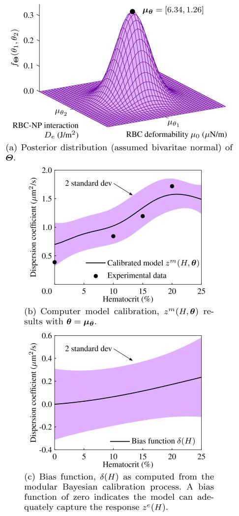
The results of different components for the modular Bayesian calibration process are shown in Fig. 8. The mean of the posterior distribution in Fig. 8(a) of θ is μ_Θ = [6.34, 1.26], and in Fig. 8(c) it is shown that the discrepancy function δ(H) from eq.(7) is approximately zero for the domain of H. A small discrepancy function indicates that the model z^e(H, θ) can adequately capture the observed experiments, as is shown for the prediction in Fig. 8(b), which is a prediction assuming the discrepancy function is zero. Consistent with intuition, however, the discrepancy function deviates from zero at higher hematocrit, which would suggest that the model is inadequate as the number of RBCs increases and interactions multiply. This may be due to the limitation of the pairwise interactions considered, the simple interactions themselves, or the interpolation scheme of the FSI model that breaks down as a higher fraction of the domain Ω becomes solid.

Fig. 8.

Components of the modular Bayesian model updating process.

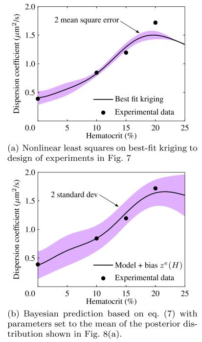
The full prediction combining the calibrated model with parameters θ set to their mean μ_Θ and the discrepancy function is shown in Fig. 9(b) along with a 2 standard deviation uncertainty band. The updated model captures the experimental data well, with the discrepancy function correctly picking up missing physics at higher hematocrit. The Bayesian method in eq. (7) is compared with a nonlinear least squares optimization of parameters θ based on a best-fit Kriging response surface (Simpson et al. 2005) applied to the same DOE in Fig. 7. In the nonlinear least square approach, the calibrated parameters are θ* = [6.80, 1.64], which are close to the mean of the posterior distribution from the Bayesian updating process. The similarity of the results provide strong evidence that the true parameters of μ₀ and D_e are around the mean of the posterior distribution in Fig. 8(a). In the next subsection, we will use μ_Θ from the posterior distribution in Fig. 8(a) because, as can be seen from the prediction in Fig. 9(b), the Bayesian approach captures the experimental observations within 2 standard deviations of the mean prediction whereas the nonlinear least squares method does not.

Fig. 9.

Comparison of Bayesian and nonlinear least squares calibration methods for blood flow simulation parameters.

3.3 Prediction of NP transport in the tumor microvasculature

Here we use the updated IFEM model to perform parametric studies that predict NP dispersion in the tumor microvasculature under uncertainty. The complex microvasculture is approximated by placing statistical models derived from experiments on the inputs to the IFEM simulation, namely the vessel diameter Y₁, flow velocity Y₂, and hematocrit Y₃ ≡ H. Each input is treated as random to account for variation among specific locations in the human body and among separate patients. The distributions of these random variables are given in Table 1. All random variables Y_i are assumed to follow lognormal distributions so that Y_i = e^B_i, where B_i are normal random variables. A lognormal random variable has parameters (m, s)_i = (μ_Bi, σ_Bi), which are also shown in the table. The value of the parameters for the lognormal distributions were calculated by the maximum likelihood method applied to data in Kamoun et al. (2010) that catalogues these parameters at different spatial locations in the microvasculature. In this simulation, we assume the random variables are independent in the tumor microvasculature, acknowledging there may be some correlation between vessel diameter and flow velocity.

Table 1.

Table describing input random variables for computational NP design under uncertainty.

Variable	Description	Distribution	Parameters
Y 1	Vessel diameter	Lognormal	(m, s)1 = (2:63; 0:087)
Y 2	Flow velocity	Lognormal	(m, s)2 = (−0:480; 0:189)
Y 3	Hematocrit	Lognormal	(m, s)3 = (−2:51; 0:269)

NPs 100 nm in diameter are simulated to estimate NP transport from the center of the vessel to the wall in the uncertain tumor microvasculature. Transport is measured by a quantity called the drift velocity, the speed with which NPs leave the vessel centerline and travel perpendicularly until they reach the vessel wall, averaged over the ensemble of NPs in the simulation. The drift velocity of particle i and their ensemble over N particles are

$$V_i=\frac{r_i\left(t\right)-r_i\left(0\right)}{t},\to \text{ensemble}V=\frac{1}{N}\sum _{i=1}^N{V}_i,$$ (11)

where r_i(t) is the distance of the NP from the center of the channel at the time t and r_i(0) is the initial value of this distance. To propagate uncertainty from the three dimensional random input space to single dimensional random output space Y ∈ (0, ∞)³ → V ∈ ℝ, we use tensor product Gauss quadrature (Lee and Chen 2009; Lee et al. 2009) so that uncertainty propagation is handled via deterministic evaluation of the drift velocity at a predetermined set of collocation points. Following (Lee et al. 2009), the ith order moment of V based on a Gauss quadrature approximation is

$$\begin{array}{cc}\hfill \langle V{\left(Y\right)}^i\rangle & ={\int }_{{\Omega }_Y}V{\left(Y\right)}^i{f}_Y\left(Y\right)dY\hfill \\ \hfill & \approx \sum _{n_1=1}^{N_1}\cdots \sum _{n_M}^{N_M}{\omega }_{n_1}\cdots {\omega }_{n_M}V{(y_{n_1},\dots ,y_{n_M})}^i,\hfill \end{array}$$ (12)

where ω_nj is the weight of the nth Gauss point of N_j total in the jth dimension of random input vector Y; the value y_nj is the location of the nth Gauss point in the jth dimension. Here, M = 3 as shown in Table 1, and we choose n_j = 2 to guarantee the predicted standard deviation of V is exact. Note that in tensor product quadrature the required number of function evaluations scales exponentially with random space dimension as n^M (if n = n₁ = n₂ = …). The nodes and weights (y, ω) can be computed based on moment matching formulae as described in (Lee et al. 2009). Moment matching equations produce a nonlinear set of equations which may be solved numerically by the Newton-Rhapson root finding method. Fig. 10 shows the Gauss nodes and weights superimposed on the probability distribution functions (PDFs) of the input random variables given in Table 1 for 3 Gauss points.

Fig. 10.

Gauss point locations and weights superimposed on the PDF of each of the input random variables Y_i to the IFEM simulation. Weights sum to 1 and the PDF parameters are given in Table 1.

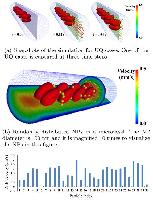
With n_j = 2, j = 1, 2, 3, a total of eight calls to the IFEM simulation are required for computing NP transport statistical moments. The drift velocity of individual NPs are predicted by the simulations results. Fig. 11(a) shows simulation snapshots for one of the 8 required input settings. In each simulation, NPs are randomly distributed at the initial time step (Fig. 11(b)). The density and the viscosity of the blood plasma are 1.0 g/cm³ and 0.0012 Pa-s, respectively. Both RBC deformability μ₀ and RBC-RBC interaction potential magnitude D_e are assigned the mean values of the posterior distribution calculated in the previous section: μ₀ = 6.34 μN/m and D_e = 1.26 μJ/m². Fig. 11(c) shows the predicted drift velocity of N = 30 NPs after 100 ms. The positive values mean the NPs are moving from the center of the channel to the wall. Most NPs have a tendency to do this. Using the moment matching formula in eq. (12), the mean drift velocity is μ_V = 3.23 μm/s and its standard deviation is σ_V = 0.95 μm/s. The dispersion coefficient was also computed with the moment matching formulae as having mean μ_DR = 0.303 μm²/s and σ_DR = 0.330 μm² /s. We note that the standard deviation of the drift velocity here is the standard deviation of the average drift velocity as computed in eq. (6), not the standard deviation of NP-specific drift velocity shown in Fig. 11(c), which was not considered in this study.

Fig. 11.

Prediction of NP transport based on the simulation model under uncertainty

4 Discussion

The results for the uncertainty propagation exercise uncover some interesting physical features of NP transport in the tumor microvasculature. First, the calculated drift velocity standard deviation corresponds to a coefficient of variation of almost 30% of the mean, which is quite large. A high coefficient of variation means that large variation of the drift velocity can be expected at different locations in the microvasculature so that NP transport design should be tailored for specific locations since they produce such different transport characteristics. Thought of another way, it is beneficial to design NPs so their dispersion characteristics are maximized in that part of the microvasculature that is of interest to their intended use such as the presence or absence of a tumor. Futhuremore, it can be used to predict the NP dispersion based on the patient-specific microvascular imaging. NP dispersion might change from patient to patient. So the optimal design of NP migth be changed. In this sense, it is possible to use the simulation method including microvascular imaging to design personailzed NPs.

The dispersion coefficient in eq. (6) produces a similar conclusion to the drift velocity above. The mean diffusion coefficient was μ_DR = 0.303 μm²/s for NPs 100 nm in diameter, which may be compared to natural diffusion as calculated by the Stokes-Einstein relation D_B = k_BT /3πμd_p, where D_B is the natural diffusion coefficient by Brownian motion, k_B is the Boltzmann constant, T is a temperature, μ is the plasma viscosity, and d_p is the particle diameter. The dispersion coefficient is lower than natural diffusion coefficient of 4.393 μm²/s at a temperature of 300 K, even considering 3 standard deviations from the mean value D_R → 1.3 μm²/s. This means that the diffusion process in the tumor microvasculature is relatively slower than the natural diffusion process, slowing to almost zero in certain areas. The natural diffusion coefficient can be a reference value for a physical sense but not sure whether NPs might diffuse to the tissue based on the natural Brownian diffusion. The current simulation shows the diffusion of NPs in the microvasculature is much less than the natural diffusion because the NP diffusion in the microvasculature has a lot of barriers such as RBCs, vessel wall, and extra cellular matrix rather than the natural diffusion in a homogeneous fluid. Therefore, the NP dispersion coefficient in the microvessel might be not the sum of natural diffusion and NP radial dispersion. Therefore, when we consider the NP transport in the tumor microvasculature, we should consider possible ways to enhance the dispersion of the particles or provide better patient-specific information about probabilities of treatment success based on locations of interest in the vasculature.

The results also suggest a use of this research for design of NP-based therapeutics. We considered predictions of statistical quantities of the average drift velocity and dispersion coefficients in the tumor microvasculature by propagating uncertainty in vessel diameter (Y₁), flow velocity (Y₂), and levels of hematocrit (Y₃). Although we conducted uncertainty propagation analysis with other model inputs fixed to traditional values, we can envision a robust design scenario (Chen et al. 1996) where medical personnel aim to design NP shape and size under uncertainty that simultaneously maximizes the mean drift velocity and minimizes the drift velocity variance in certain regions. This would correspond to minimizing the following objective function:

$$\underset{x}{\max }f(x,Y)=-w{\mu }_v(x,Y)+(1-w){\sigma }_v(x,Y),$$ (13)

where ω ∈ [0, 1] defines the weight assigned to the mean term, μ_V is the mean of the average dispersion coefficient, σ_V is the standard deviation of the average dispersion coefficient, Y are the random variables in Table 1, and x = [x₁, x₂] are the design variables: NP major axis size and NP aspect ratio, respectively. The support of random variables Y should be adjusted to reflect the random conditions in specific portions of the microvasculature. The robust design formulation in eq. (13) recognizes a tradeo between the mean NP drift velocity and its variance. In short, we do not aim only to maximize V but also ensure that the value of V at the optimum design point will be insensitive to input uncertainties. This ensures that NP drug delivery treatments are effective for different patients or tumors located at different sites in the human body.

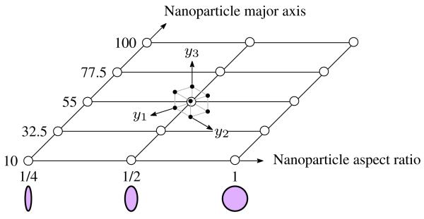
To perform the optimization in eq. (13), which either requires gradient evaluation or random sampling of the objective function, we must replace the costly blood flow simulation with a response surface (Jin et al. 2001). The same tensor product grid uncertainty propagation approach used in previous Section can be applied at a design of experiments on x₁, x₂. This concept is shown in Fig. 12, which may be visualized as a moment-matching stochastic collocation sampling space surrounding each discrete point in the design domain. A separate response surface for μ_v and σ_v would then be built in the x domain in eq. (13) and optimization techniques performed to determine the optimum NP shape and size. This exercise is left to future work but rests on the foundational concepts promulgated in this research: the recognition and mathematical quantification of uncertainty in NP transport phenomena in the microvasculature as a pre-requisite to targeted NP-based therapeutics and bio-sensing.

Fig. 12.

Design of experiments for computational design under uncertainty. The design variables x in eq. (13) are treated deterministically while noise parameters y are treated random. The tensor product quadrature cube for noise parameter samples is superimposed on one of the design points.

References

- Bayarri MJ, Berger JO, Paulo R, Sacks J, Cafeo JA, Cavendish J, Lin CH, Tu J. A framework for validation of computer models. Technometrics. 2007;49(2):138–254. [Google Scholar]
- Cabral H, Matsumoto Y, Mizuno K, Chen Q, Murakami M, Kimura M, Terada Y, Kano MR, Miyazono K, Uesaka M, Nishiyama N, Kataoka K. Accumulation of sub-100 nm polymeric micelles in poorly permeable tumours depends on size. Nature Nanotechnology. 2011;6(12):815–823. doi: 10.1038/nnano.2011.166. [DOI] [PubMed] [Google Scholar]
- Chauhan VP, Stylianopoulos T, Martin JD, Popovic Z, Chen O, Kamoun WS, Bawendi MG, Fukumura D, Jain RK. Normalization of tumour blood vessels improves the delivery of nanomedicines in a size-dependent manner. Nature nanotechnology. 2012;7(6):383–388. doi: 10.1038/nnano.2012.45. [DOI] [PMC free article] [PubMed] [Google Scholar]
- Chen W, Allen JK, Tsui KL, Mistree F. A procedure for robust design: Minimizing variations caused by noise factors and control factors. ASME Journal of Mechanical Design. 1996;118(4):478–485. [Google Scholar]
- Dao M, Lim CT, Suresh S. Mechanics of the human red blood cell deformed by optical tweezers. Journal of the Mechanics and Physics of Solids. 2003;51(1112):2259–2280. [Google Scholar]
- Decuzzi P, Godin B, Tanaka T, Lee SY, Chiappini C, Liu X, Ferrari M. Size and shape effects in the biodistribution of intravascularly injected particles. Journal of Controlled Release. 2010;141(3):320–327. doi: 10.1016/j.jconrel.2009.10.014. [DOI] [PubMed] [Google Scholar]
- Duncan R. Polymer conjugates as anticancer nanomedicines. Nature Reviews Cancer. 2006;6(9):688–701. doi: 10.1038/nrc1958. [DOI] [PubMed] [Google Scholar]
- Ferrari M. Cancer nanotechnology: opportunities and challenges. Nature Reviews Cancer. 2005;5(3):161–171. doi: 10.1038/nrc1566. [DOI] [PubMed] [Google Scholar]
- Jin R, Chen W, Simpson TW. Comparative studies of metamodelling techniques under multiple modelling criteria. Structural and Multidisciplinary Optimization. 2001;23(1):1–13. [Google Scholar]
- Jin R, Chen W, Sudjianto A. An efficient algorithm for constructing optimal design of computer experiments. Journal of Statistical Planning and Inference. 2005;134(1):268–287. [Google Scholar]
- Kamoun WS, Chae S, Lacorre DA, Tyrrell JA, Mitre M, Gillissen MA, Fukumura D, Jain RK, Munn LL. Simultaneous measurement of rbc velocity, flux, hematocrit and shear rate in vascular networks. Nature Methods. 2010;7(8):655–660. doi: 10.1038/nmeth.1475. [DOI] [PMC free article] [PubMed] [Google Scholar]
- Kennedy MC, O’Hagan A. Bayesian calibration of computer models. Journal of the Royal Statistical Society: Series B (Statistical Methodology) 2001;63(3):425–464. [Google Scholar]
- Kopacz AM, Liu WK. Immersed molecular electrokinetic finite element method. Computational Mechanics. 2013 doi: 10.1039/c2nr31279d. in press. [DOI] [PubMed] [Google Scholar]
- Kopacz AM, Patankar NA, Liu WK. The immersed molecular finite element method. Computer Methods in Applied Mechanics and Engineering. 2012;233-236:28–39. [Google Scholar]
- Lee S, Chen W. A comparative study of uncertainty propagation methods for black-box-type problems. Structural and Multidisciplinary Optimization. 2009;37(3):239–253. [Google Scholar]
- Lee S, Chen W, Kwak B. Robust design with arbitrary distributions using gauss-type quadrature formula. Structural and Multidisciplinary Optimization. 2009;39(3):227–243. [Google Scholar]
- Lee TR, Chang YS, Choi JB, Kim DW, Liu WK, Kim YJ. Immersed finite element method for rigid body motions in the incompressible navierstokes flow. Computer Methods in Applied Mechanics and Engineering. 2008;197(2528):2305–2316. [Google Scholar]
- Lee TR, Choi M, Kopacz AM, Yun SH, Decuzzi P, Liu WK. Near-wall accumulation of nanoparticles in the microcirculation: smaller is not better. 2013 doi: 10.1038/srep02079. submitted. [DOI] [PMC free article] [PubMed] [Google Scholar]
- Liu WK, Liu Y, Farrell D, Zhang L, Wang XS, Fukui Y, Patankar N, Zhang Y, Bajaj C, Lee J, Hong J, Chen X, Hsu H. Immersed finite element method and its applications to biological systems. Computer Methods in Applied Mechanics and Engineering. 2006;195(1316):1722–1749. doi: 10.1016/j.cma.2005.05.049. [DOI] [PMC free article] [PubMed] [Google Scholar]
- Liu WK, Kim DW, Tang S. Mathematical foundations of the immersed finite element method. Computational Mechanics. 2007a;39(3):211–222. [Google Scholar]
- Liu Y, Liu WK. Rheology of red blood cell aggregation by computer simulation. Journal of Computational Physics. 2006;220(1):139–154. [Google Scholar]
- Liu Y, Liu WK, Belytschko T, Patankar N, To AC, Kopacz A, Chung JH. Immersed electrokinetic finite element method. International Journal for Numerical Methods in Engineering. 2007b;71(4):379–405. [Google Scholar]
- Namdee K, Thompson AJ, Charoenphol P, Eniola-Adefeso O. Margination propensity of vascular-targeted spheres from blood flow in a microfluidic model of human microvessels. Langmuir. 2013;29:2530–2535. doi: 10.1021/la304746p. [DOI] [PubMed] [Google Scholar]
- Park Y, Best C, Kuriabova T, Henle ML, Feld MS, Levine AJ, Popescu G. Measurement of the nonlinear elasticity of red blood cell membranes. Phys Rev E. 2011;83:051,925. doi: 10.1103/PhysRevE.83.051925. [DOI] [PMC free article] [PubMed] [Google Scholar]
- Peer D, Karp JM, Hong S, Farokhzad OC, Margalit R, Langer R. Nanocarriers as an emerging platform for cancer therapy. Nature nanotechnology. 2007;2(12):751–760. doi: 10.1038/nnano.2007.387. [DOI] [PubMed] [Google Scholar]
- Saadatmand M, Ishikawa T, Matsuki N, Abdekhodaie M, Imai Y, Ueno H, Yamaguchi T. Fluid particle diffusion through high-hematocrit blood flow within a capillary tube. Journal of Biomechanics. 2011;44(1):170–175. doi: 10.1016/j.jbiomech.2010.09.004. [DOI] [PubMed] [Google Scholar]
- Simpson TW, Martin JD, Booker AJ, Giunta AA, Haftka RT, Renaud JE, Kleijnen JPC. Use of kriging models to approximate deterministic computer models. AIAA Journal. 2005;43(4):853–863. [Google Scholar]
- Sinek J, Sanga S, Zheng X, Frieboes H, Ferrari M, Cristini V. Predicting drug pharmacokinetics and effect in vascularized tumors using computer simulation. Journal of Mathematical Biology. 2009;58:485–510. doi: 10.1007/s00285-008-0214-y. [DOI] [PMC free article] [PubMed] [Google Scholar]
- Tan J, Thomas A, Liu Y. Influence of red blood cells on nanoparticle targeted delivery in microcirculation. Soft Matter. 2012;8:1934–1946. doi: 10.1039/C2SM06391C. [DOI] [PMC free article] [PubMed] [Google Scholar]
- van de Ven AL, Kim P, Haley O, Fakhoury JR, Adriani G, Schmulen J, Moloney P, Hussain F, Ferrari M, Liu X, Yun SH, Decuzzi P. Rapid tumoritropic accumulation of systemically injected plateloid particles and their biodistribution. Journal of Controlled Release. 2012;158(1):148–155. doi: 10.1016/j.jconrel.2011.10.021. [DOI] [PMC free article] [PubMed] [Google Scholar]
- Zhang J, Johnson P, Popel AS. Red blood cell aggregation and dissociation in shear flows simulated by lattice boltzmann method. Journal of Biomechanics. 2008;41(1):47–55. doi: 10.1016/j.jbiomech.2007.07.020. [DOI] [PMC free article] [PubMed] [Google Scholar]
- Zhang L, Gerstenberger A, Wang X, Liu WK. Immersed finite element method. Computer Methods in Applied Mechanics and Engineering. 2004;193(2122):2051–2067. [Google Scholar]