Abstract
We investigate using dual time-point PET data to perform Patlak modeling. This approach can be used for whole body dynamic PET studies in which we compute voxel-wise estimates of Patlak parameters using two frames of data for each bed position. Our approach directly uses list-mode arrival times for each event to estimate the Patlak parametric image. We use a penalized likelihood method in which the penalty function uses spatially variant weighting to ensure a count independent local impulse response. We evaluate performance of the method in comparison to fractional changes in SUV values (%DSUV) between the two frames using Cramer Rao analysis and Monte Carlo simulation. Receiver operating characteristic (ROC) curves are used to compare performance in differentiating tumors relative to background based on the dynamic data sets. Using area under the ROC curve as a performance metric, we show superior performance of Patlak relative to %DSUV over a range of dynamic data sets and parameters. These results suggest that Patlak analysis may be appropriate for analysis of dual time-point whole body PET data and could lead to superior detection of tumors relative to %DSUV metrics.
Keywords: Whole body, Patlak, dynamic PET, lesion detection, SUV, dual time-point
Introduction
POSITRON emission tomography (PET) is a powerful technique for staging cancer and assessing response to therapy. Whole body FDG (18F-Fludeoxyglucose) imaging is among the most common clinical protocols in which the patient is stepped through the scanner so that a 3D volumetric image of the whole body can be reconstructed. These “static” images represent accumulated tracer uptake at the time of scanning (typically 1 hour post injection) and are of clinical value for detection and semiquantitative analysis of primary tumors and metastatic lesions. However, static PET imaging does not exploit the full potential of this inherently dynamic modality. An alternative approach is to acquire data continuously from the time the tracer is administered and to then fit a kinetic model [1]. These models allow us to represent tracer uptake in terms of quantitative rate parameters which have the potential for improved tumor characterization compared to more widely used semi-quantitative measures such as the SUV (standardized uptake value) [2].
Standard whole body and dynamic imaging protocols are inconsistent with each other since one requires imaging at multiple positions while the other requires acquisition of complete dynamic data at a single position. In this paper we develop an image estimation approach that could be used for dynamic whole body imaging. To achieve this goal we use the Patlak method [3], a simplified kinetic model for irreversibly bound tracers such as FDG, and we estimate the parameters of this model from partial dynamic data consisting of short frames of data acquired over two disjoint observation periods. Whole body data can then be acquired at two different time points for each bed position and the Patlak model fitted separately for each bed position. The resulting images can then be stitched together to form a quantitative whole body dynamic image.
Dynamic models are frequently fit to a sequence of reconstructed images with one set of parameters computed for data averaged over a user selected region of interest. An alternative approach, and that adopted here, is to directly fit the data to a kinetic model at each voxel in the image. This idea was first proposed by Snyder [4] in 1984. Since then several maximum likelihood [5], [6], [7] and penalized ML [8], [9] methods have been described for this purpose. The rate parameters in these kinetic models are nonlinearly related to the data and result in nonconvex optimization problems. Furthermore, the relatively high dimensionality of the search space (four per voxel for the two compartment model typically used for FDG) can result in instability of the estimates and high computation cost, limiting the use of these direct estimators.
The simplified Patlak model, applicable when tracers are irreversibly trapped in the second compartment (k4 = 0), uses an approximation that models the measured time activity curve in steady state as a weighted sum of the input function and its integral. The weights are referred to respectively as the Patlak slope and intercept. The slope in particular is a physiologically meaningful quantity representing the net transfer rate or influx constant and could be used in place of SUV values as a biomarker. For example, Graham et al. [10] found that Patlak slope is a better predictor of outcome and a better discriminator between normal tissue and tumor than SUV after comparing them in a group of 40 patients with colon cancer metastasized to the liver. We note that the Patlak approximation is only valid for irreversible trapping, which is not always the case for FDG. For example, Iozzo et al [11] show nonzero k4 in liver. However, in practice the Patlak model is frequently and effectively used in studies of tumor viability.
Wang et al. [12] described a penalized ML method for voxel-wise reconstruction of Patlak parameters using a preconditioned conjugate gradient method applied to a sequence of frames. We developed an alternative penalized ML approach that uses list-mode rather than binned data [13]. In that case, as in the current paper, we used an incremental gradient algorithm originally developed for nonparametric dynamic imaging with a B-spline temporal basis [14]. Here we investigate a modified version of this algorithm that uses list-mode data from two acquisition frames. Preliminary versions of this work were reported in [13] and [15].
The concept of using two-pass whole body scans is not new, but has been extensively studied in the context of SUV values. These studies look at changes in SUV value between two acquisition frames, typically expressed as percent fractional difference: %DSUV = 100 * (SUV2 − SUV1)/SUV1. By using fractional changes, these measures become invariant to the scaling by dose and body-weight used in standard SUV. For this reason %DSUV reflects only dynamic changes in uptake and is robust to the uncertainties governing the relationship between FDG uptake and patient weight that make standard SUV values only semi-quantitative. Alkhawaldeh et al. [16] found that dual time-point PET can improve diagnostic accuracy relative to standard single frame SUV, increasing sensitivity and specificity for malignant lung nodules diagnostic, especially for small lung lesions that have low SUVs. Prieto et al. [17] showed that dual time-point PET can improve sensitivity for the identification and volume delineation of high-grade brain tumors compared with standard PET studies. Hu et al. [18] reported that for mediastinal nodal staging, the specificity, accuracy, and positive predictive value of dual time-point scans were better than those of single-time-point by adding extra %DSUV information. Zhuang et al. [19] and Kumar et al. [20] found that malignant lesions showed a significant increase in SUV over time, while benign lesions showed a decrease. As a result, %DSUV can have advantages over SUV in differentiating malignant from benign lesions. However, negative results have also been reported: Cloran et al. [21] reported that dual time-point FDG PET may not be of benefit in the assessment of pulmonary nodules with maximum SUV of less than 2.5 on initial imaging. Chan et al. [22] suggested that dual time-point FDG-PET does not improve the overall evaluation of pulmonary lesions. In the studies presented below we perform comparisons between our Patlak based method and %DSUV since both can make use of identical dual time-point data.
Recently, Karakatsanis [23], [24] proposed a clinical protocol for wholebody Patlak estimation composed of an initial 6min dynamic scan over the heart followed by a sequence of PET scans (6-pass × 7 bed position each). The Patlak image estimate is obtained by applying a hybrid linear regression model to the temporal static images. Their work also aims at the quantification of tracer dynamics with the Patlak model, with results indicating the advantage of Patlak modeling over SUV. This differs from our approach, both in the use of multiple bed frames per bed position and in the estimation of Patlak images from reconstructed static images. The use of multiple frames per bed position may limit the practical utility of this approach.
The paper is organized as follows: we first introduce the list-model Patlak model and image reconstruction methods in Sections 2.1.1 and 2.1.2. We then derive an expression for the Cramer Rao bounds on the Patlak parameters in Section 2.2. The problem of ensuring count-independent resolution in the penalized ML images is addressed in Section 2.3. Results presented in Section 3 include Cramer-Rao analysis (Section 3.1) and lesion detectability studies (Section 3.2) for a simplified single detector pair/single voxel model. In Section 3.3 we present a volumetric imaging simulation and comparison with %DSUV and demonstrate the performance of our count-independent resolution method in Section 3.4. We conclude with a discussion of the performance of the method and its extensions to processing of clinical whole body data in Section 4.
Method
In this section we first formulate our Patlak approach using penalized maximum likelihood estimation from list-mode PET data. We then derive the Cramer-Rao bound for an unbiased estimator of the Patlak parameters, which provides a quick means to investigate lower bounds on the variance of the estimator as a function of the parameters of the acquisition protocol. Using this result we can compare the best-case performance of our list-mode algorithm with alternatives including sinogram-based Patlak estimation and lesion detection using %DSUV. Finally we derive a spatially-variant weighting penalty that enforces count independent resolution in the reconstructed Patlak images. Use of this weighting ensures that the resolution of the Patlak slope and intercept are matched, and also that resolution does not vary across the image due to spatial variation in activity. Using the algorithm and analysis developed in this section we are then able to investigate the performance of dual time-point Patlak estimation under a range of conditions and in comparison to the alternative approaches of sinogram-based estimation and %DSUV.
2.1 Patlak Estimation from two Frame List-Mode Data
2.1.1. Patlak List-Mode Likelihood
The Patlak model provides an approximate solution to the two compartment kinetic model for irreversible tracers in the steady state period t ≥ T0 in which changes are effectively due to irreversible trapping in a single compartment. Let η(t) be the tracer time activity curve (TAC) with blood input function C(t). We can write the Patlak equation as [12], [13]:
| (1) |
where κ is the net influx rate or slope parameter, and q is the intercept of the Patlak model. Our goal is to compute estimates of κ and q at each voxel in the source space from list-mode data.
Using the Patlak model, we can represent the rate function at voxel j after steady state t ≥ T0 as a linear combination of two basis functions B1(t) and B2(t):
| (2) |
where . We note that since the basis function B1(t) is the integral of B2(t), the two functions will always be linearly independent. The rate function in the measured sinogram space at line of response (LOR) i can be written as:
| (3) |
where the exponential term accounts for radioactive decay of the tracer with half-life τLog(2); pij is the probability of an event at voxel j being detected at detector pair i; and nv is the number of voxels. The additional terms ri(t) and Si(t) denote, respectively, the randoms and scattered coincidence rate functions. This formulation is the same as that used in our earlier work on continuous time reconstruction from list-mode data [25] except that here we use the input function and its integral rather than cubic b-splines as the temporal basis. In the following we use a factored system model for pij based on a product of attenuation factors, normalization, geometric response, and a Monte Carlo model of the detector response as described in [26]. We assume that random and scatter rate functions are estimated prior to image reconstruction and that they are separable into spatial and temporal factors as described in [25].
Assuming we have continuous list-mode data over time interval [T0, T] and the arrival times in the list-mode data follow an inhomogeneous Poisson model, the continuous time log-likelihood function of event arrival times is given by:
| (4) |
where aik denotes the arrival time of the k’ th photon at detector pair i, xi is the number of events detected in LOR i, and np is the total number of LORs. In the case when we collect data over two subintervals [T1 T2] and [T3 T4] we have:
| (5) |
where the aik are constrained to those events detected in the intervals [T1 T2] and [T3 T4]. In principal we can use this formulation to investigate behavior for a single frame or for an arbitrarily large number. However, our goal in this work is to focus on a practical approach to whole body dynamic imaging so we consider only the two frame case. Two frame data could be acquired using similar protocols now used for %DSUV methods in which the patient is scanned twice in each bed position.
2.1.2 Patlak Image Estimation
To compute images of the Patlak slope and intercept parameters we regularize the log-likelihood function with a quadratic spatial penalty function:
| (6) |
where w = wjl is a 2nv length vector containing the Patlak slope and intercept image values for each voxel; wjl is indexed by voxel index j = 1, …. nv, and basis l = 1,2 (for slope and intercept respectively). RS is a 2nv × 2nv matrix that computes the weighted squared pairwise difference between each voxel and its 26 nearest neighbors separately for both slope and intercept images.
The spatial penalty for our problem can be written as
| (7) |
where the weights µjl,j′l can either (i) define a shift invariant penalty by setting them equal to the inverse of the Euclidean distance between the two voxels, or (ii) be precomputed from the data to ensure count independent resolution in the Patlak slope and intercept image as we describe below in Section 2.3.
This formulation is very similar to that described in our work on list-mode based reconstruction of continuous time dynamic images [25], with the main difference being the use of the Patlak basis functions in place of a cubic b-spline basis. Consequently, we can compute solutions using the same numerical optimization procedure. Here we use the 4D incremental gradient method we describe in [14]. This algorithm iterates over subsets of data in such a way as to ensure convergence to a maximum of F(W) in (6). The update equation for this algorithm has the form:
| (8) |
where n denotes the iteration number, m denotes the subiteration number, fm denotes the mth sub-objective function, D(wn,m−1) is a diagonal preconditioning matrix, and Pτ is a projection operator used to ensure convergence to a local maximum. Unlike the full parametric model, the Patlak formulation results in a concave cost function so that any local maximum is a global maximum. We refer readers to the details in [14] for a complete description of the algorithm and update equations.
2.2 The Cramer-Rao Lower Bound
To gain insight into the potential performance of this approach from the perspective of estimating Patlak parameters from limited data, we computed Cramer Rao lower bounds (CRLBs) on these parameters. While we give the general expression for the CRLBs below, in Section III we explore the bounds only for the simplified case of a single LOR and a single voxel. In that case, a spatial penalty is not required to obtain a stable estimate so that we might expect that bounds computed from the un-penalized log likelihood will reflect the actual variances seen in our estimators. We will examine the bias and variance of the estimator further in Section III using Monte Carlo simulation.
The CRLB provides a lower bound on the variance of any unbiased estimator of the Patlak parameters. The bounds are found from the inverse of the Fisher information matrix (FIM) defined as
| (9) |
where m and n are voxel indices, and j and l are the indices of the basis functions (j,l=1,2). Rather than directly derive the closed-form CRLB for the list-mode likelihood (5), as we do in [15], we instead use the bin-mode likelihood approximation described in [27]. In this approximation we assume data are binned into multiple sinograms so that in the limit as the frame duration goes to zero, the sinogram likelihood converges to that of the list-mode data.
In the closely related problem of direct estimation of Patlak parameters from sinogram PET data [12], the log-likelihood function can be written as:
| (10) |
where is the mean number of events over the sinogram, λi(t) is the rate function as in (3), and yi is the number of detected events between the ith detector pair. The partial derivatives of L(W)are
| (11) |
where we write B̃j(t) and B̃l(t) as decay corrected basis functions, i.e. B̃j(t) = e−t/τBj(t) and B̃l(t) = e−t/τBl(t). Taking the expectation we obtain the single frame sinogram FIM:
| (12) |
To find the FIM for single frame list-mode data we use the bin-mode approximation of the log-likelihood function (4) by assuming the data are binned into a large number of sinograms nt each of duration Δt:
| (13) |
where λi(t) is the rate function as in (3) and nt is the number of time bins with t1 = T0 and tnt = T. Taking partial derivatives of L(W) leads to
| (14) |
Taking the expectation gives:
| (15) |
Finally, in the limit as Δt → 0, we have
| (16) |
This result extends directly to the two frame case as:
| (17) |
We have compared numerical values computed using the approximate finite sum over n = 1,..nt in (15) to those found using the more complex closed-form expression in [15] and found negligible differences for values of nt > 100 We use the expression (15) to compute the CRLBs for the studies described in Section 3.2.
2.3 Enforcing Count Independent Resolution in Patlak Images
It is well known that using a spatially invariant penalty function with a Poisson likelihood leads to a count-dependent image resolution [28]. This is because noise variance scales with mean number of counts, causing the smoothing effect of the penalty function to also be count dependent. This issue has previously been addressed using a spatially variant weighting function for static reconstruction [28], [29], [30]. Asma and Leahy [27] extended this approach to ensure count and temporally invariant resolution in reconstruction of dynamic images. Here we describe a modification of the approach in [31] to develop a spatially variant weighting function to ensure that resolution in the Patlak images is count independent.
As we describe below, resolution is a function of the FIM. We again use the bin-mode approximation of the list-mode likelihood from which we then derive an approximate expression for the local impulse response of the penalized maximum likelihood estimates of the Patlak images. This approximate expression is a function of the product of the Fisher information and the weights µjl,j′l in (7) and we can therefore locally vary these weights to ensure count independent resolution.
The local impulse response (LIR) at voxel j corresponds to the mean change in the reconstructed image in response to a perturbation of the true source distribution at that pixel. In the case of linear estimators this corresponds to the standard source-independent impulse response of the system. However, for nonlinear estimators the LIR is dependent on the underlying source distribution. As shown in [28] and further investigated in [29], the LIR at voxel j and the covariance matrix for penalized ML estimation of the form (6) can be approximated respectively as:
| (18) |
| (19 |
Where w̃ is the estimated Patlak image, F is the FIM, ej is the unit vector at voxel j ∈ {1,2,..,2nv}, and Rs is the quadratic penalty function with β a global (scalar) smoothing parameter.
Again following [31], the bin-mode approximation of the FIM in (15) can be written in matrix form as:
| (20) |
where ⊗ denotes the Kronecker product, is a diagonal matrix with element (in, in) equal to the reciprocal of the mean of the data at LOR i in time bin n, P is the system matrix introduced in (3), and B is a decay corrected temporal basis function matrix of dimension nt by 2 whose (n,l)th element is given by . Note here the matrix representation assumes a finite number of time bins.
To compute the LIR based on (18) we need to find a tractable approximation to the inverse of the FIM. We begin with the approximation originally due to Fessler et al. [28] and used for dynamic reconstruction in [31]:
| (21) |
where we use the identity (P ⊗ B)T(P ⊗ B) = (PTP) ⊗ (BTB) . Dκ ≡ D{kjl}, Dv ≡ D{vjl} are diagonal matrices with elements:
| (22) |
| (23) |
Note that in writing the integrals in (22) and (23) we are taking the limit as Δt → 0, in the bin mode likelihood, as we do in (16). Similarly, in the limit, the matrix BTB has the form:
| (24) |
The approximation given by (21) is based on the observation that the Fisher information matrix is concentrated along its diagonal so that a reasonable approximation should at least match the diagonal elements. Substituting (22) and (23) in (21), it is straightforward to show that the diagonal values of (21) match those of (20).
Denoting where θjl = kjl/vjl, we can plug the FIM representation (21) directly into (18) and (19) to obtain the expression for the LIR at each voxel:
| (25) |
Noting that Dθ ejl = θjl ejl and using the property (ABA)−1 = A−1 B−1 A−1 we can rewrite (25) as
| (26) |
And similarly the covariance is:
| (27) |
While (26) and (27) can be used to investigate the properties of images reconstructed using the method described above, here we are specifically concerned with modifying the penalty function (7) so as to ensure approximately count invariant resolution.
The LIR is by construction a measure of local blurring around voxel j. The factors in (22) and (23) tend to vary slowly in the vicinity of any voxel j so that we can locally approximate θjlDθ−1 ≈ I. The matrix PTP associated with combined forward and backprojection is approximately locally spatially shift invariant, and BTB is dependent on the temporal bases only and therefore strictly spatially shift invariant. Consequently the matrix PTP ⊗ BTB can be regarded as approximately spatially shift invariant. It follows that to achieve approximate count and shift invariance in the LIR it is sufficient for the term βDθ−1 RsDθ−1 in (26) to be independent of the true source distribution and spatially shift invariant.
Suppose we select the weights µjl,j′l in (7) such that we can write
| (28) |
where Řs is a spatially invariant operator. Then we would have:
| (29) |
| (30) |
which gives us the desired count and shift invariant LIR for the Patlak slope and intercept images. We would also like to achieve matched resolution between the Patlak slope and intercept. With reference to (29) it follows that this can be achieved with a circulant matrix BTB. We can achieve this by scaling the basis function B̃2(t) by
| (31) |
With this scaling the diagonal elements in (24) are equal so that the LIR will have the same height for both slope and intercept images. After reconstruction the intercept image is then multiplied by 1/α to find the correctly scaled values. It now remains to determine the weights µjl,j′l such that Řs has the desired invariant property. Before proceeding we note that with the spatial invariance in Řs the LIR does still depend on β, which is desirable as it gives us a single parameter with which to control the trade-off between noise and resolution. We note also that while this method should produce invariance to count rates, there will still be some variation in spatial resolution. The reason for this is that the intrinsic resolution of PET scanners, and therefore the matrix PTP, is slowly spatially variant, with decreasing radial resolution in the transaxial plane as one moves away from the central axis of the scanner. Since we do not compensate for this in the above analysis, we will see a similar radial dependence in resolution as we move away from the center of the field of view. It is possible to also compensate for this effect, as described in [26], but this causes noise variance to increase away from the center of the field of view, and in practice it is preferable to allow this small decrease in resolution rather than amplifying noise.
From the definition of the penalty function in (7) we can write
| (32) |
where Sl(j,j′) = 2 Σj"∈Nj,µjl,j"l if j = j′ and −2µjl,j"l if j ≠ j′ for l = 1,2 and j,j′ = 1, …. nv. Similarly, the modified matrix in (28) has the form:
| (33) |
where
Note that setting
| (34) |
where Ejj′ is the Euclidean distance between the two voxels results in a value Šl(j,j′) = −2/Ejj′, for all off-diagonal elements in the neighborhood Nj of each pixel j and zero elsewhere. For the diagonal elements we then have values
| (35) |
Again, under the observation that locally θjl varies slowly, this value is approximately Šl(j,j′) = 2 Σj"∈Nj 1/Ejj". For a regular (shift invariant) neighborhood system this will result in the matrix Řs having the shift invariant behavior we are attempting to impose.
To conclude, the appropriate weights to use in the penalty function to assure approximate count independent resolution in the reconstructed images are µjl,j′l = 1/θjlθj′lEjj′ where
| (36) |
On modifying the bin-mode likelihood function in (17) to include the two separate acquisition frames: [T1, T2] and [T3, T4]), it is straightforward to show that 0, has the following form:
| (37) |
Similarly the correct scaling of B̃2(t) to match resolution between the slope and intercept images for two frame data is:
| (38) |
Results
3.1 Cramer Rao Analysis
To explore the potential performance of dual time-point Patlak imaging we use the FIM expressions derived above to compute CR bounds on the estimated Patlak parameters. The CR bound provides a lower bound on the variance of any unbiased estimator of a parameter. In practice these bounds are frequently tight and reflect the achievable variance of maximum likelihood estimators. In the following we first compare CR bounds with estimator variances computed using Monte Carlo simulation to show that the bounds are tight. We then use these results as the basis for a comparison of lesion detection performance based on dual time-point imaging using our Patlak approach in comparison to fractional SUV. Since the difference between fractional SUV and Patlak analysis lies largely in the handling of the dynamic rather than the spatial information, we can obtain insight into the problem through consideration of a simplified problem corresponding to a single image voxel from which we directly observe Poisson counts generated according to the dynamic TAC associated with a particular model.
We used a two compartment model with irreversible trapping in the second compartment, κ4 = 0. The studies reported in the following subsections used the range of kinetic parameters listed in Table 1 for tumor and background, which were found in the literature on Patlak modeling [32–39].
Table 1.
11 Pairs of kinetic model parameters for background and tumors identified in the literature [32], [33], [34], [35], [36], [37], [38], [39].
| Tumor region kinetics | Normal tissue kinetics | |||||
|---|---|---|---|---|---|---|
| Set | K1 ml/g /min |
k2 ml/g /min |
k3 ml/g /min |
K1 ml/g /min |
k2 ml/g /min |
k3 ml/g /min |
| 1 | 0.198 | 0.228 | 0.035 | 0.533 | 0.980 | 0.012 |
| 2 | 0.076 | 0.134 | 0.115 | 0.194 | 0.557 | 0.054 |
| 3 | 0.088 | 0.091 | 0.037 | 0.117 | 0.176 | 0.008 |
| 4 | 0.062 | 0.055 | 0.074 | 0.719 | 0.788 | 0.003 |
| 5 | 0.057 | 0.045 | 0.077 | 0.889 | 1.062 | 0.004 |
| 6 | 0.069 | 0.029 | 0.121 | 0.845 | 1.019 | 0.004 |
| 7 | 0.075 | 0.078 | 0.080 | 0.708 | 0.865 | 0.004 |
| 8 | 0.076 | 0.042 | 0.082 | 0.786 | 0.750 | 0.004 |
| 9 | 0.064 | 0.061 | 0.078 | 1.151 | 1.348 | 0.007 |
| 10 | 0.110 | 0.084 | 0.062 | 0.452 | 0.589 | 0.006 |
| 11 | 0.149 | 0.041 | 0.098 | 1.251 | 1.325 | 0.009 |
We used the FIM expressions from Section 2.2 to compute Cramer-Rao bounds for the kinetic parameters and compared these to maximum likelihood (ML) parameters estimated from data simulated for each model. In this single voxel/detector model no smoothing penalty is required and parameters were estimated by maximizing the likelihood function (5). The data were simulated by generating arrival times for photons corresponding to a time inhomogeneous Poisson process defined by the TAC for each parameter set for a realistic input function. We included scatter proportional to the true rate and randoms proportion to the square of the true rate, each scaled to contribute at 30% of the mean true counts when averaged over the entire TAC. In practice, randoms and scatter are spatially smooth relative to the trues, as we simulate in Section 3.3. In that case, the scatter and randoms TACs will have a different shape than those of the trues. However, for this 1D example we make the simplifying assumption that the randoms and scatter dynamics follow trues as described above. To compute the bounds, the mean random and scatter rates were assumed known. We then retained those arrival times corresponding to the two frames: 40–45mins and 80–85mins. Different count levels were achieved by scaling the input function. We performed 100,000 Monte Carlo trials for each parameter set and computed the mean and standard deviation (s.d.) for these trials for the Patlak slope parameter.
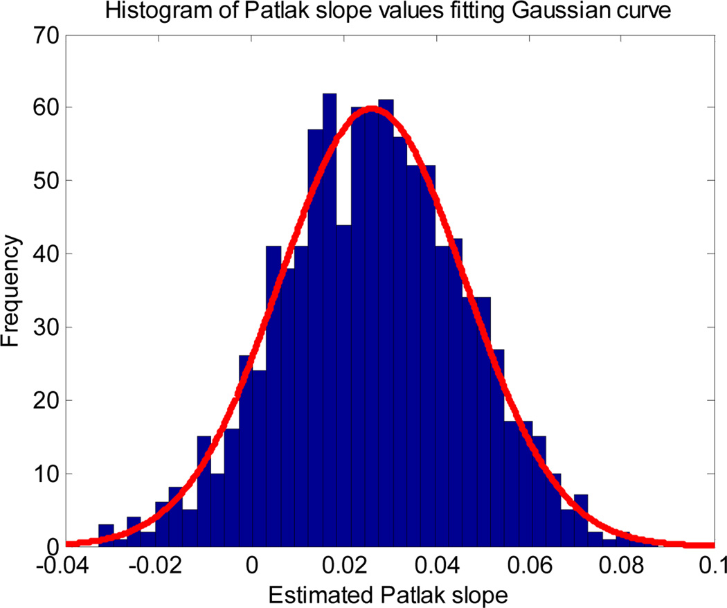
Table 2 compares the CR bound and standard deviation of Patlak slope for the tumor kinetic parameters in the first row of Table 1. The true value of Patlak slope for these parameters is .0262/min. For all count levels the error in the mean from the ML estimator is less than 0.5%. Therefore we can regard the estimator as effectively unbiased. This is consistent with the asymptotically unbiased property of the maximum likelihood estimator. The CR variance bounds are within 2% of the corresponding Monte Carlo values. Consequently it is reasonable to use the CR bound as a closed form estimate of the standard deviation of ML estimated parameters as we do in the following subsection. In the following we also use the fact that the ML estimators approximately follow a Gaussian distribution. This property is illustrated in Fig.1 which shows the sample distribution of the Patlak slope parameters for one parameter set for 1,000 Monte Carlo trials overlaid with a Gaussian with matched mean and variance.
Table 2.
Comparison of the s.d. of Patlak slope obtained from the CR bound with mean and s.d. computed by Monte Carlo simulation with maximum likelihood parameter estimation.
| Count level | 1 | 2 | 3 | 4 | 5 |
|---|---|---|---|---|---|
| Mean tumor counts |
59.8 | 69.8 | 79.7 | 89.7 | 99.7 |
| Mean of Monte Carlo Patlak slope |
0.0262 | 0.0263 | 0.0262 | 0.0262 | 0.0263 |
| Cramer Rao lower bound (s.d.) |
0.0143 | 0.0133 | 0.0124 | 0.0117 | 0.0111 |
| Monte Carlo (s.d.) |
0.0145 | 0.0134 | 0.0125 | 0.0119 | 0.0112 |
Fig. 1.
Histogram of the estimated Patlak slope fitting a Gaussian curve.
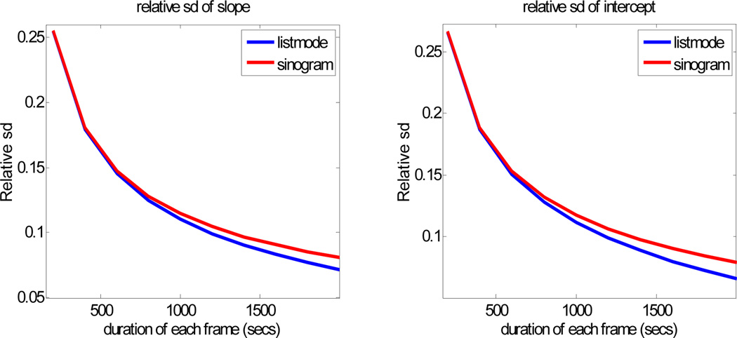
We also used Cramer-Rao analysis to compare Patlak estimation from two frame list-mode vs. two frames of binned sinogram data. Again, we used the single voxel model with Cramer-Rao values computed using the FIM based on the bin-mode approximation (15) for list-mode data, and the two-frame extension of (12) for the sinogram data. Figure 2 shows standard deviations for the two estimators as a function of frame duration. The starting time for the 2 frames was fixed at 40 and 80min using parameters from the first row in Table 1. As one might expect, the methods are matched for shorter frame duration, but the list-mode method improves relative to sinogram data as duration increases.
Fig. 2.
Relative standard deviation of Patlak slope and intercept for list-mode and sinogram based estimation method with different duration of acquisition frames.
3.2 ROC Analysis: Dual Time-Point Patlak vs. Fractional SUV
Using the results of the preceding analysis we next performed a Receiver Operating Characteristic (ROC) study to determine the relative performance of dual time-point Patlak and fractional SUV in differentiating tumor from background. We again used the single voxel/detector model described above.
To compute ROC curves we find the distribution of the Patlak slope parameter estimates for tumor and background. The ROC curve is then formed by plotting the rate of true positive vs. false positive tumor detection as a function of the threshold applied to the Patlak parameter.
For comparison we also computed ROC curves for fractional SUV:
| (39) |
where C1 and C2 are the ML estimates of activity in each of the two frames (note that the normalization factors used to compute SUV values from calibrated PET images cancel in the fractional SUV model so aren’t considered here). With the dual time-point imaging protocol, many researchers have used %DSUV as a common approach while the absolute difference of SUV values is not generally used [40], [18], [19] since these values are sensitive to normalization. Similarly, in our experiments we restrict our attention to %DSUV in comparison with the Patlak method. For the single voxel/detector model the ML estimator for a static frame is equal to the number of counts observed over the frame. To determine the distribution of %DSUV we used the Monte Carlo simulation method outlined above with 10,000 repetitions and computed the sample distribution.
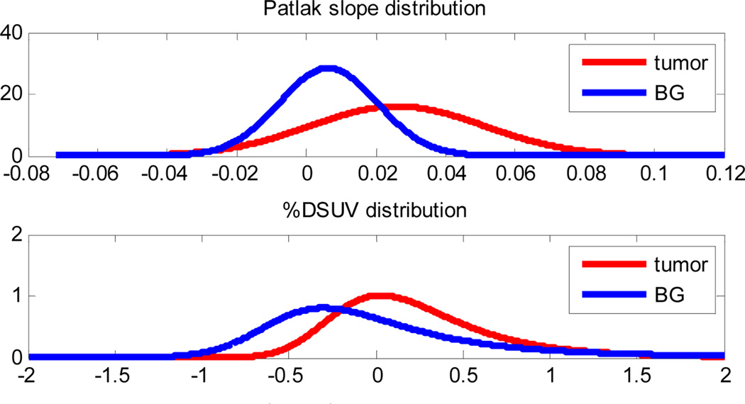
Examples of the distributions with kinetic parameter set 1 from Table 1 are shown in Fig. 3 with ROC areas 0.7565 and 0.5166 for Patlak and %DSUV respectively.
Fig. 3.
An example of the distribution of Patlak slope parameter (upper) and %DSUV (lower) for tumor and background (BG).
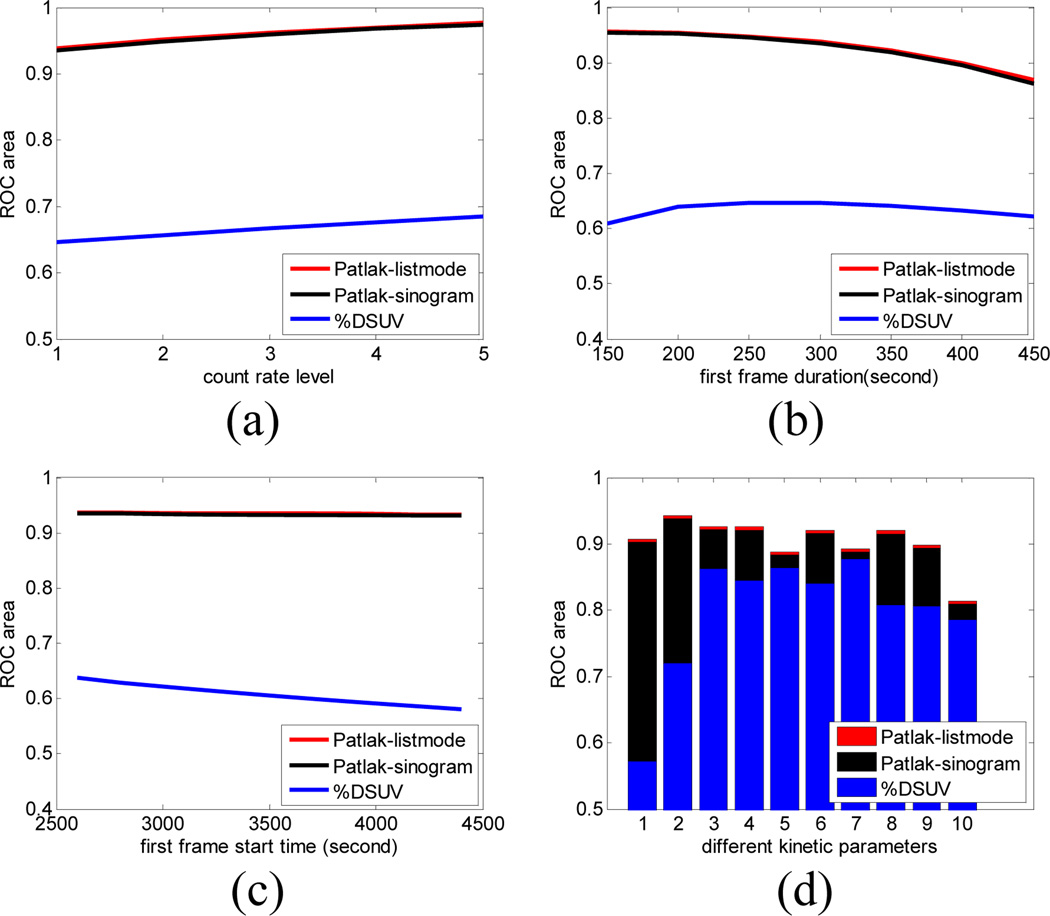
We repeated the same procedure for a range of different count rates, frame durations and acquisition start times, in each case computing the area under the ROC curve for the Patlak slope and %DSUV measures. In each case, randoms and scatters were added to the data. Area under the ROC curves was computed using the CR analysis described above for both list-mode and sinogram based Patlak estimation. These are shown relative to %DSUV analysis in Fig. 4. Figure 4 upper left shows ROC areas for 5 different count levels for parameters equal to the first row of Table 1 with two 5min frames starting at 40min and 80min respectively. Figure 4 upper right shows ROC areas for the lowest count level in Table 2 with acquisition again beginning at 40 and 80mins. In this case we kept the total acquisition to 10min but varied the relative duration of the first and second frames. Figure 4 lower left keeps the same count rate and total duration and 40min inter-frame interval, but varies the starting point for the first frame. Figure 4 lower right shows the ROC areas for Patlak and %DSUV for all kinetic parameter sets except the first row in Table 1 for two 10min frames beginning at 40 and 80mins and a count rate approximately equal to the lowest value reported in Table 2.
Fig. 4.
Detection of tumors relative to background using rate parameters from Table 1. We compare area under ROC curves (AUC) for Patlak slope (sinogram and list-mode based estimation) and %DSUV as a function of (a) count rate, (b) duration of first frame, and (c) first frame start time. Panel (d) shows the area under the ROC curves averaged over simulations for different parameter sets listed in Table 1.
From Fig 4. we see that list-mode based estimation slightly outperforms the sinogram based method in terms of the AUC, although the differences are small. These results indicate there is little difference in performance between list-mode and sinogram based estimation for the range of parameters tested here. However the fact that the list-mode approach always performs as well or better than sinogram based estumation supports its use in subsequent studies.
We also observe consistently better performance in distinguishing tumor and background with Patlak compared to %DSUV even though both methods use the same data. Since %DSUV has already shown advantages over SUV in cancer staging as we have reviewed in the introduction, these results are promising indications of practical utility for our dual time-point strategy in whole body cancer imaging. These simulations also may provide guidance for optimizing scan parameters for two frame imaging. By extending these simulations to a wider range of parameters we can optimize start times for the two frames and their relative duration give a fixed total scan time so as to maximize area under the ROC curve.
3.3 Simulated Imaging Studies
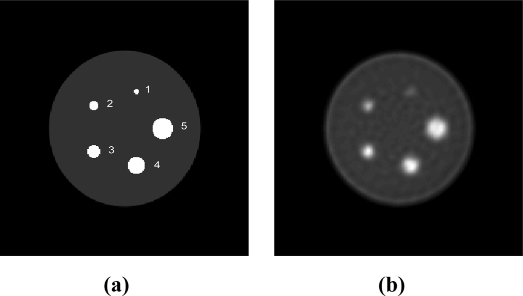
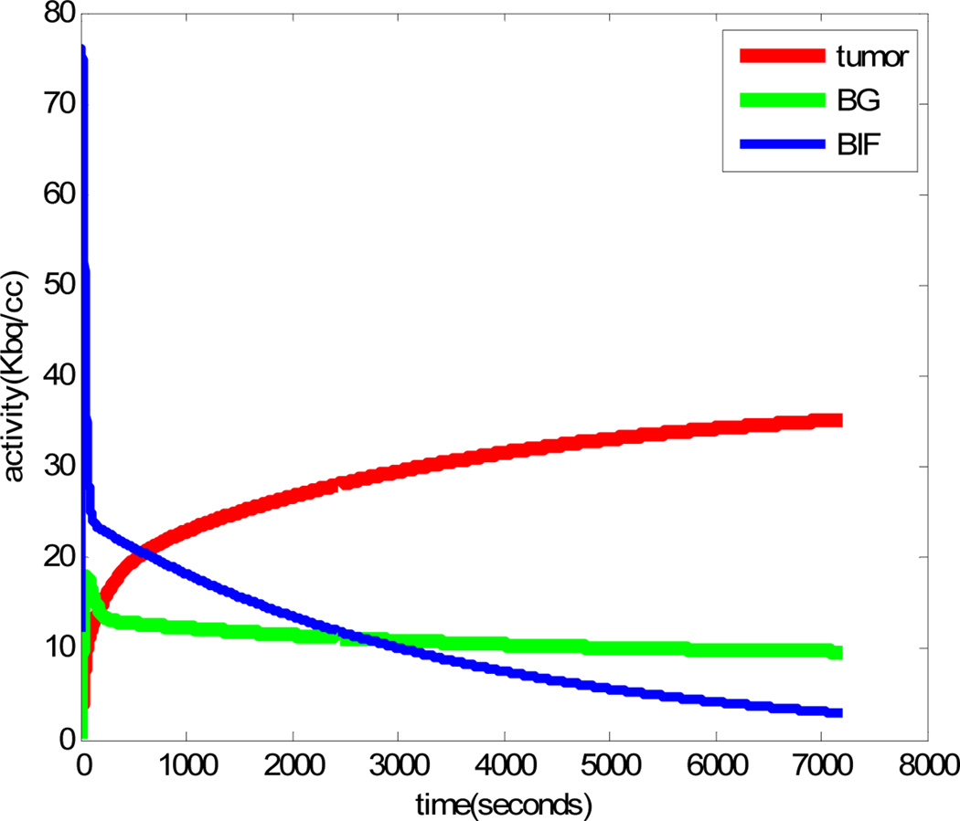
For these studies we simulated a small scale 3D PET system (diameter: 148.4mm, detector size: 2.423mm × 2.423mm; number of rings: 4) with a total of 13 2D sinograms each with 84 angles of view by 96 radial LORs. A uniform cylinder phantom of diameter 31.4mm is centered in the scanner and contains 5 cylinders (“tumors”) of diameter 1.0, 1.8, 2.6, 3.4, and 4.2mm as shown in Fig. 5(a). We simulated time activity curves for tumors and background using the first set of kinetic parameters in Table 1. The blood input function, tumor and background TACs are shown in Fig. 6. As in the Cramer Rao analysis, we added scatters and randoms to the data. Both processes were assumed to be separable, with the temporal variation in scatter and randoms proportional respectively to the instantaneous true and squared-true activity integrated over all LORs. Total activity contributed by the scatters and randoms were both set at 30% of the total true activity. The mean number of total counts for the following studies over the entire scanning time was 17M. The TACs for each sinogram element are computed by forward projection through a system matrix generated for the scanner using the model described in [26]. Each of these TACs represents the time-inhomogeneous Poisson processes that determine emission rates for each LOR. List-mode data are then generated by sampling from these TACs. In the results presented here, we window the data to retain only those events corresponding to two five minute frames starting at 40min and 80min. We generated a total of 100 trials for our Monte Carlo simulations. We used the modified 4D incremental gradient (4DIG) algorithm [13] to reconstruct the Patlak slope and intercept images as described in Section 2. The mean of the Patlak slope images over the 100 trials is shown in Fig. 5b. We also computed static penalized ML reconstructions of each frame using the method described in [26] with spatially variant smoothing to ensure count independent resolution as described in [30]. To ensure a fair comparison we matched resolution of the static and Patlak images as described below in Section 3.5.
Fig. 5.
(a) Uniform cylinder (“background”) with 5 cylinders (“tumor”) of different sizes, (b) The mean (over 100 Monte Carlo trials) of the Patlak slope image reconstructed from two 5min frame list-mode data starting at 40min and 80min with TACs as in Fig. 6.
Fig. 6.
Simulated time-activity-curves for tumor, background and the blood input function with kinetic parameters from row 1 in Table 1.
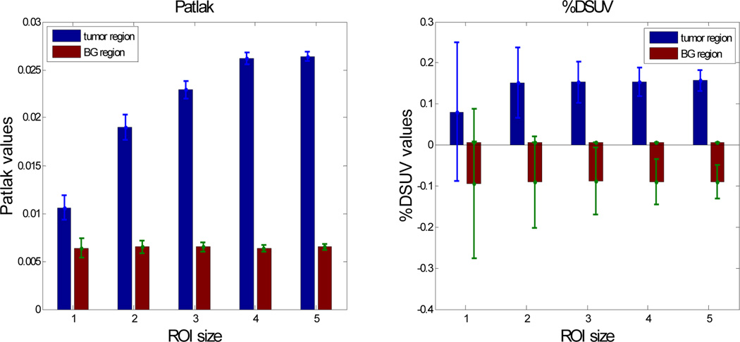
For each of the 100 trials we computed the average Patlak slope parameter for each of 5 tumor regions of interest (ROIs) and 5 corresponding background ROIs with sizes matching those of the tumor ROIs. Similarly we computed the mean intensity in each ROI for each static reconstruction and then computed %DSUV values. The mean and s.d. results for Patlak and %DSUV for each of the five ROIs are shown in Fig. 7.
Fig. 7.
Mean and s.d. (error bars) for each of five ROIs shown in Fig. 5(a) for list-mode Patlak and %DSUV. %DSUV values were computed by applying (39) to activity in each frame after averaging over the ROI.
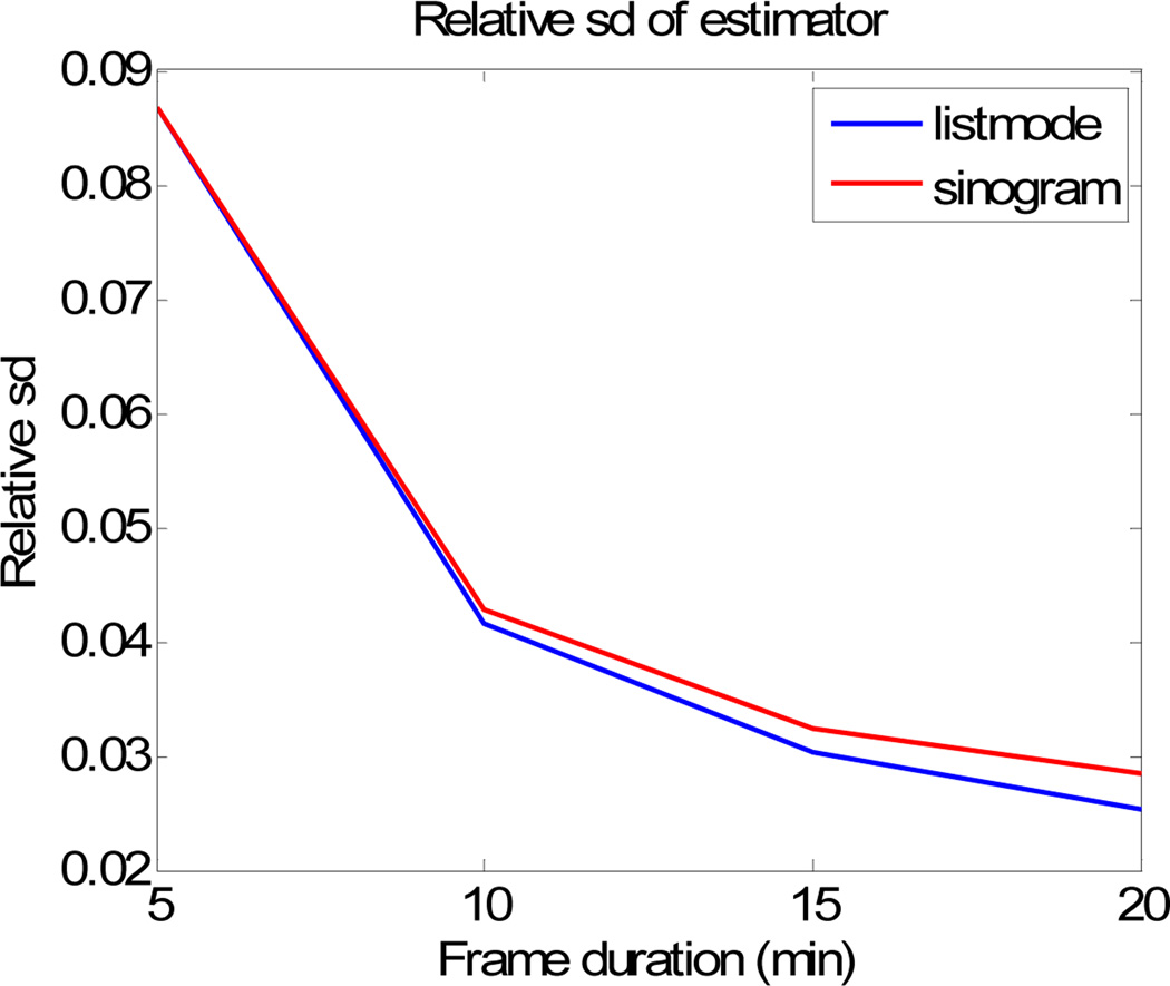
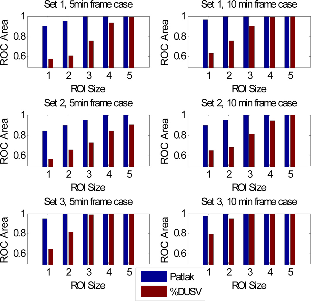
As a comparison between list-mode and sinogram based Patlak estimation, we compute the standard deviation of the mean Patlak slope within the biggest tumor. The results are displayed in Fig. 8. The relative sd of the list-mode based estimation is uniformly smaller than that of the sinogram based method, which is consistent with what we observe in the Cramer Rao analysis. Assuming Gaussian distributions for the ROI means in each case, we computed areas under the ROC curve for detection of each of the “tumors” relative to a size-matched background ROI. These results are shown in Fig. 9. In this figure we include ROC results for Monte Carlo simulations for parameters corresponding to the first three rows in Table 1 and include results for 10min as well as 5min frames.
Fig. 8.
Relative sd of Patlak slope estimate computed from 100 Monte-Carlo trials for the biggest tumor region.
Fig. 9.
Area under the ROC curve for kinetic parameter sets 1, 2, 3 in Table 1 for Patlak and %DSUV based tumor detection. See text for details.
We see that as the size of the ROI increases, s.d. in %DSUV drops in Fig. 7 leading to improving ROC values in Fig. 9 with increasing ROI size. In the Patlak case, the performance also improves as ROI size increases, but overall the s.d.’s are far lower than in the %DSUV images so that ROC results are considerably better for the smaller ROIs. These results are consistent with our earlier single voxel/detector study and again indicate potential benefits of using Patlak over %DSUV for detection, especially for smaller tumors.
3.4 Enforcing Count-Invariant Resolution
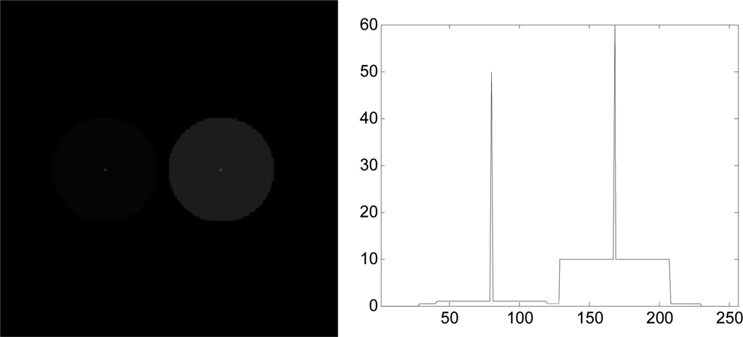
To investigate the effectiveness of our technique to ensure count-invariant resolution we simulated a cool cylindrical background with one hot and one warm smaller cylinder insert, each with a point source at their center. The entire phantom has the same dynamic activity curve at each voxel but with the relative scale point source: hot cylinder : warm cylinder : background of 50 : 10 : 1 : 0.4. The phantom and a profile through the 2 point sources are shown in Fig. 10.
Fig. 10.
(left) Digital phantom for validating count-independent resolution and (b) profile through the 2 point sources in the phantom
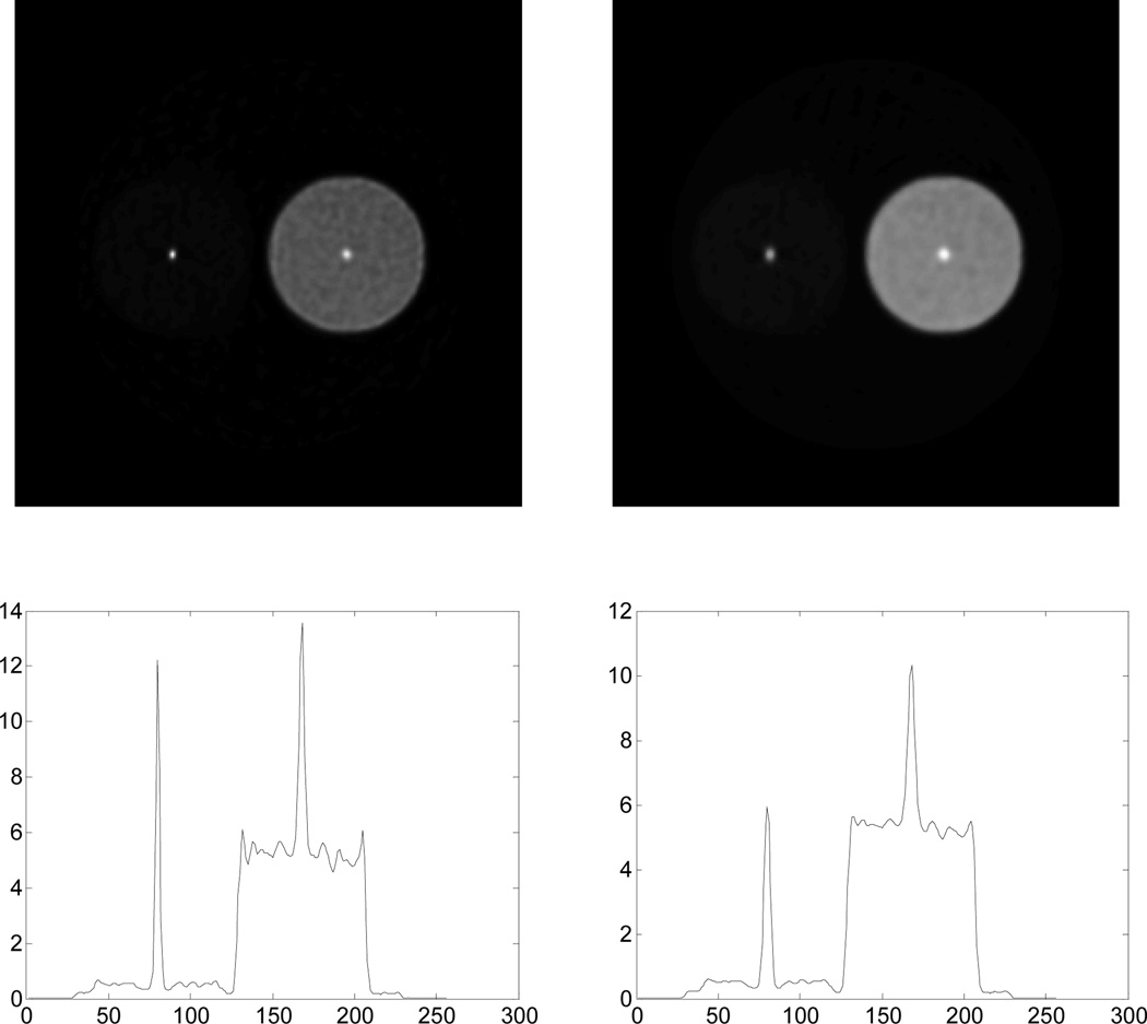
We simulated data for this phantom using the same method as described in Section 3.3. Randoms and scatters were added to the true events as described above. The data for the entire acquisition time was 23M counts. We then reconstructed images of Patlak slope and intercept using the count-invariant spatial weighting of the smoothing penalty defined in (37) and, for comparison, a spatial weighting equal to the inverse of the Euclidean distance between each pair of pixels. The reconstructed Patlak slope image and a profile for one noisy reconstruction using these two different penalties are shown in Fig. 11. The figure shows that the reconstructed height of the two point sources is quite different using the spatially invariant weighting but approximately equal when using the count-dependent spatially variant weighting.
Fig. 11.
Profiles through one reconstructed Patlak slope image with (left) spatially invariant smoothing and (right) spatially variant smoothing for count-independent resolution using (37).
To explore this performance quantitatively we computed the peak value of the local impulse response at the location of the point source in the hot and warm cylinders as a measure of contrast recovery coefficient (CRC). These values are tabulated for Patlak slope and intercept in Table 3 for three different values of the global smoothing parameter β when using a uniform spatial weight for the penalty term. These results clearly show that the hot and warm cylinders have differing CRCs for each value of β. Furthermore, the slope and intercept also have distinct CRCs. In contrast, for the same data using a shift-variant weighting we obtain CRCs that are approximately equal in the hot and warm cylinders for both the slope and intercept images for each value of β as shown in Table 4. Furthermore, we see that after modifying the count rate for this study from low to high, we again obtain CRCs that are invariant for fixed β and approximately equal for both the high and low count rates.
Table 3.
CRC at 2 point sources for the low count level and the uniform spatial penalty.
| Beta | 0.1 | 0.5 | 1 | ||||
|---|---|---|---|---|---|---|---|
| Warm | Hot | Warm | Hot | Warm | Hot | ||
| Low Count |
slope | 0.430 | 0.418 | 0.311 | 0.258 | 0.236 | 0.191 |
| Inter | 0.460 | 0.532 | 0.450 | 0.465 | 0.429 | 0.433 | |
Table 4.
CRC at 2 point sources for low and high count levels and our modified spatial penalty.
| Beta | 0.1 | 0.5 | 1 | ||||
|---|---|---|---|---|---|---|---|
| Warm | Hot | Warm | Hot | Warm | Hot | ||
| Low Count |
slope | 0.471 | 0.469 | 0.428 | 0.434 | 0.350 | 0.352 |
| inter | 0.467 | 0.472 | 0.437 | 0.437 | 0.363 | 0.367 | |
| High Count |
slope | 0.478 | 0.512 | 0.448 | 0.449 | 0.374 | 0.372 |
| inter | 0.475 | 0.514 | 0.470 | 0.483 | 0.421 | 0.440 | |
3.5 Matching Resolution in Patlak and %DSUV images
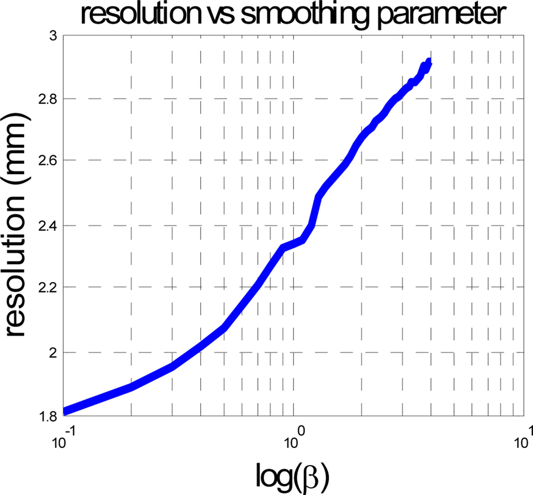
To make the comparisons in Section 3.3 meaningful it is important that the resolution of the Patlak and static images from which we computed %DSUV values are matched. The penalized ML static images were reconstructed using the spatially variant smoothing method described in [30]. This ensures that resolution is matched in the two frames in each dual frame study and further that it can be controlled using a single parameter which plays the same role as the β parameter in the Patlak image smoothing function in (6) and (21). We computed a calibration curve of β vs. full width at half maximum (FWHM) resolution as shown in Fig. 12. The curve is based on the approximation that the mean of the reconstructed image equals the reconstruction of the mean of the data [28]. We therefore reconstruct noiseless data for a point source at the center of the field of view and then compute the FWHM resolution for multiple different values of the smoothing parameter β to obtain the curve in Fig. 12.
Fig. 12.
Resolution v.s. log of smoothing parameter β in static MAP reconstructions computed at the center of hot tumor for the phantom in Fig. 5
The resolution of the Patlak parametric image vs β cannot be obtained from the mean of the data because we are using a list-mode likelihood function that depends on the individual arrival times. Rather than modify the algorithm to compute resolution based on bin-mode likelihood we used a Monte Carlo method to empirically determine resolution. We computed the FWHM resolution for the mean image averaged over the 100 Monte Carlo trials described above for the point source at the center of the hot tumor for the phantom in Fig. 5. The resolution was measured to be 2.05mm. We then found the β value that matched this resolution in the static images and use this for all of the studies reported in Section 3.3. A more complete study would also investigate the relative performance of %DSUV and Patlak methods as a function resolution parameter β, however the primary difference between the two methods is the manner in which the dynamic data is handled. Both use the same spatial model so we would expect relative performance to be somewhat robust to changes in resolution. Limited simulation studies we have performed but not included here appear to support this conjecture.
DISCUSSION AND CONCLUSIONS
The ROC results in Section 3.1 show that for a single data/single voxel Cramer-Rao study over a wide range of parameter values, Patlak slope estimates from dual time-point data consistently out-perform fractional SUV measures computed from the same data. The advantage of the Cramer-Rao approach is that we can rapidly evaluate performance for many different acquisition parameters. Consequently in addition to comparisons to fraction SUV, we can also use this approach to optimize acquisition in terms of start and end times for the two frames when designing whole body protocols.
Our analysis of resolution in Section 2.3 provides the theoretical basis for modifying the cost function to ensure that reconstructed Patlak images have a resolution that does not depend on activity or count rate and furthermore that the resolution of the slope and intercept parameters are matched. This is important for the purposes of qualitative and quantitative interpretation of the Patlak values. For example, matched resolutions allow meaningfull comparisons of Patlak slope values, which are inevitably affected by partial volume effects for small lesions, across subjects and over time for a single subject. Removing dependence on activity will make these values more reliable biomarkers that can potentially be used for staging and assessing response to therapy.
The simulated imaging studies in Section 3.3 make use of the count-independent resolution method to compare performance of Patlak and fractional SUV methods at matched resolutions. Through Monte Carlo simulation over a range of lesion sizes, we see in Figs. 7 and 9 that, as with the Cramer Rao analysis, Patlak slope parameters are more accurate in differentiating tumor and background than is fraction SUV. This is particularly the case for the smaller lesions where the much smaller relative variance of Patlak measures lead to better differentiation of tumor and background.
In summary, the results presented in Section 3 support the conjecture that Patlak values estimated from dual time-point PET data can produce more meaningful indications of tracer dynamics than are extracted using the fractional SUV approach. Comparisons of list-mode and sinogram based Patlak image estimation show little difference for short (5min) duration frames but with improvements in list-mode performance relative to sinograms as the duration increases. In practice there may be little difference in performance between the two approaches, but the list-mode approach always performs at least as well as the sinogram method.
Our reason for pursing the two time-point method, rather than the more standard method of acquiring a full dynamic scan, is that we plan to extend this approach to whole body studies where the patient must be stepped through the scanner to produce the whole body image. The method described in this paper is directly applicable to two time-point whole body data.
In principle, data acquisition for whole body Patlak imaging requires a simple modification of current whole body protocols in that the patient is simply stepped through the scanner twice rather than once. However, a number of practical issues arise in acquiring and processing this data. First there needs to be a delay of 40–60mins between frames. Assuming 5mins per bed position and 5 positions to cover the patient, the patient must remain in the scanner for 65–85mins. It is difficult to remain stationary for that long, so that coregistration between frames will be needed when processing practically acquired data. A second complication is that a blood input function is required. Arterial sampling is not practical for the envisioned application, but a population or model based approach can be applied for this purpose. Finally, the usual calibrations for attenuation, scatter, randoms and system sensitivity need to be included when implementing this method for experimental whole body data. Methods for addressing these practical issues, and the resulting whole body reconstructions, will be described in a future publication.
Acknowledgments
This work was supported by NIH grants R01EB013293, R21 CA149587 and R01EB010197.
Footnotes
Personal use of this material is permitted. However, permission to use this material for any other purposes must be obtained from the IEEE by sending a request to pubs-permissions@ieee.org.
Contributor Information
Wentao Zhu, Signal and Image Processing Institute, University of Southern California, LA, CA 90089 USA.
Quanzheng Li, Massachusetts General Hospital, Boston, MA, 02114 USA.
Bing Bai, Department of Radiology, University of Southern California, LA, CA 90089 USA.
Peter S. Conti, Department of Radiology, University of Southern California, LA, CA 90089 USA
Richard M. Leahy, Email: leahy@sipi.usc.edu, Signal and Image Processing Institute, University of Southern California, LA, CA 90089 USA.
References
- 1.Carson RE. Tracer kinetic modeling in PET. In: Valk PE, et al., editors. Positron Emission Tomography, Basic Science and Clinical Practice. London: Springer; 2002. pp. 127–159. [Google Scholar]
- 2.Zasadny KR, Wahl RL. Standardized uptake values of normal tissues at PET with 2-[fluorine-18]-fluoro-2-deoxy-D-glucose: variations with body weight and a method for correction. Radiology. 1993;189:847–850. doi: 10.1148/radiology.189.3.8234714. [DOI] [PubMed] [Google Scholar]
- 3.Patlak CS, Blasberg RG, Fenstermacher JD. Graphical evaluation of blood-to-brain transfer constants from multiple-time uptake data. Journal of Cerebral Blood Flow and Metabolism. 1983;2(1):1–7. doi: 10.1038/jcbfm.1983.1. [DOI] [PubMed] [Google Scholar]
- 4.Snyder DL. Parameter Estimation for Dynamic Studies in Emission-Tomography Systems Having List-Mode Data. Nuclear Science, IEEE Transactions on. 1984;31(2):925–931. [Google Scholar]
- 5.Carson RE, Lange K. The EM parameter image reconstruction algorithm. J. Amer. Statist. Assoc. 1985;80(389):20–22. [Google Scholar]
- 6.Reader AJ, Sureau FC, Comtat C, Trébossen R, Buvat I. Joint estimation of dynamic PET images and temporal basis functions using fully 4D ML-EM. Physics in Medicine and Biology. 2006;51(21):5455–5474. doi: 10.1088/0031-9155/51/21/005. [DOI] [PubMed] [Google Scholar]
- 7.Matthews J, Bailey D, Price P, Cunningham Y. The direct calculation of parametric images from dynamic PET data using maximum-likelihood iterative reconstruction. Physics in Medicine and Biology. 1997;42(6):1155–1173. doi: 10.1088/0031-9155/42/6/012. [DOI] [PubMed] [Google Scholar]
- 8.Kamasak ME, Bouman CA, Morris ED, Sauer K. Direct reconstruction of kinetic parameter images from dynamic PET data. IEEE Trans Med Imag. 2005;24(5):636–650. doi: 10.1109/TMI.2005.845317. [DOI] [PubMed] [Google Scholar]
- 9.Wang G, Qi J. Generalized Algorithms for Direct Reconstruction of Parametric Images From Dynamic PET Data. Medical Imaging, IEEE Transactions on. 2009:1717–1726. doi: 10.1109/TMI.2009.2021851. [DOI] [PMC free article] [PubMed] [Google Scholar]
- 10.Graham MM, Peterson LM, Hayward M. Comparison of simplified quantitative analyses of FDG uptake. Nucl Med Biol. 2000;27(7):647–655. doi: 10.1016/s0969-8051(00)00143-8. [DOI] [PubMed] [Google Scholar]
- 11.Iozzo P, Geisler F, Oikonen V, Mäki M, Takala T, Soli O, Ferrannini E, Knuuti J, Nuutila P. Insulin Stimulates Liver Glucose Uptake in Humans: An 18 F-FDG PET Study. J Nucl Med. 2003;44(5):682–689. [PubMed] [Google Scholar]
- 12.Wang G, Fu L, Qi J. Maximum a posteriori reconstruction of Patlak parametric image from sinograms in dynamic PET. Physics in Medicine and Biology. 2008;53:593–604. doi: 10.1088/0031-9155/53/3/006. [DOI] [PubMed] [Google Scholar]
- 13.Li Q, Leahy RM. Direct Estimation of Patlak Parameters from List Mode PET Data. Biomedical Imaging: From Nano to Macro, ISBI '09. IEEE International Symposium on. 2009:390–393. [Google Scholar]
- 14.Li Q, Asma E, Ahn S, Leahy RM. A Fast Fully 4D Incremental Gradient Reconstruction Algorithm for List Mode PET Data. IEEE Trans. Med. Imag. 2007;26(1):58–67. doi: 10.1109/TMI.2006.884208. [DOI] [PubMed] [Google Scholar]
- 15.Zhu W, Li Q, Leahy RM. Dual-time-point Patlak estimation from list mode PET data. Biomedical Imaging (ISBI), 2012 9th IEEE International Symposium on. 2012:486–489. [Google Scholar]
- 16.Alkhawaldeh K, Bural G, Kumar R, Alavi A. Impact of dual-time-point 18F-FDG PET imaging and partial volume correction in the assessment of solitary pulmonary nodules. Eur J Nucl Med Mol Imaging. 2008;35(2):246–252. doi: 10.1007/s00259-007-0584-1. [DOI] [PubMed] [Google Scholar]
- 17.Prieto E, Martí-Climent J, Domínguez-Prado J, Garrastachu P, Díez-Valle R, Tejada S, Aristu J, Peñuelas I, Arbizu J. Voxel-based analysis of dual-time-point 18F-FDG PET images for brain tumor identification and delineation. J Nucl Med. 2011;52(6):865–872. doi: 10.2967/jnumed.110.085324. [DOI] [PubMed] [Google Scholar]
- 18.Hu M, Han A, Xing L, Yang W, Fu Z, Huang C, Zhang P, Kong L, Yu J. Value of dual-time-point FDG PET/CT for mediastinal nodal staging in non-small-cell lung cancer patients with lung comorbidity. Clin Nucl Med. 2011;36(6):429–433. doi: 10.1097/RLU.0b013e3182173810. [DOI] [PubMed] [Google Scholar]
- 19.Zhuang H, Pourdehnad M, Lambright ES, Yamamoto AJ, Lanuti M, Li P, Mozley PD, Rossman MD, Albelda SM, Alavi A. Dual Time Point 18F-FDG PET Imaging for Differentiating Malignant from Inflammatory Processes. J Nucl Med. 2001;42(9):1412–1417. [PubMed] [Google Scholar]
- 20.Kumar R, Loving VA, Chauhan A, Zhuang H, Mitchell S, Alavi A. Potential of Dual-Time-Point Imaging to Improve Breast Cancer Diagnosis with 18F-FDG PET. J Nucl Med. 2005;46(11):1819–1824. [PubMed] [Google Scholar]
- 21.Cloran FJ, Banks KP, Song WS, Kim Y, Bradley YC. Limitations of dual time point PET in the assessment of lung nodules with low FDG avidity. Lung Cancer. 2010;68(1):66–71. doi: 10.1016/j.lungcan.2009.05.013. [DOI] [PubMed] [Google Scholar]
- 22.Chan WL, Ramsay SC, Szeto ER, Freund J, Pohlen JM, Tarlinton LC, Young A, Hickey A, Dura R. Dual-time-point (18)F-FDG-PET/CT imaging in the assessment of suspected malignancy. J Med Imaging Radiat Oncol. 2011;55(4):379–390. doi: 10.1111/j.1754-9485.2011.02287.x. [DOI] [PubMed] [Google Scholar]
- 23.Karakatsanis NA, Lodge MA, Tahari AK, Zhou Y, Wahl RL, RA Dynamic whole-body PET parametric imaging: I. Concept, acquisition protocol optimization and clinical application. Physics in Medicine and Biology. 2013;58(29):7391–7418. doi: 10.1088/0031-9155/58/20/7391. [DOI] [PMC free article] [PubMed] [Google Scholar]
- 24.Karakatsanis NA, Lodge MA, Tahari AK, Zhou Y, Wahl RL, RA Dynamic whole-body PET parametric imaging: II. Task-oriented statistical estimation. Physics in Medicine and Biology. 2013;58(20):7419–7445. doi: 10.1088/0031-9155/58/20/7419. [DOI] [PMC free article] [PubMed] [Google Scholar]
- 25.Nichols TE, Qi J, Asma E, Leahy RM. Spatiotemporal Reconstruction of List Mode PET Data. IEEE Trans Med Imag. 2002;21(4):396–404. doi: 10.1109/TMI.2002.1000263. [DOI] [PubMed] [Google Scholar]
- 26.Qi J, Leahy RM, Cherry SR, Chatziioannou A, Farquhar TH. High Resolution 3D Bayesian Image Reconstruction Using the MicroPET Small-animal Scanner. Physics in Medicine and Biology. 1998;43(4):1001–1013. doi: 10.1088/0031-9155/43/4/027. [DOI] [PubMed] [Google Scholar]
- 27.Asma E, Leahy RM. Temporally invariant uniform spatial resolution in dynamic PET. Nuclear Science Symposium Conference Record, IEEE. 2003;5:3092–3096. [Google Scholar]
- 28.Fessler JA, Rogers WL. Spatial resolution properties of penalized-likelihood image reconstruction: space-invariant tomographs. IEEE Trans Image Process. 1996;5(9):1346–1358. doi: 10.1109/83.535846. [DOI] [PubMed] [Google Scholar]
- 29.Qi J, Leahy RM. Resolution and noise properties of MAP reconstructions in fully 3D PET. IEEE Trans. Medical Imaging. 2000;19(5):493–506. doi: 10.1109/42.870259. [DOI] [PubMed] [Google Scholar]
- 30.Li Q, Bai B, S. C, Smith A, Leahy RM. Count independent resolution and its calibration. Proc. 10th Fully 3D Image Recon. Meeting. 2009 [Google Scholar]
- 31.Asma E, Leahy RM. Mean and covariance properties of dynamic PET data reconstructions from list-mode data. IEEE Trans. Med. Imag. 2006;25(1):42–54. doi: 10.1109/TMI.2005.859716. [DOI] [PubMed] [Google Scholar]
- 32.Schiepers C, Chen W, Dahlbom M, Cloughesy T, Hoh CK, Huang SC. 18F-fluorothymidine kinetics of malignant brain tumors. Eur J Nucl Med Mol Imaging. 2007;34(7):1003–1011. doi: 10.1007/s00259-006-0354-5. [DOI] [PubMed] [Google Scholar]
- 33.Nishiyama Y, Yamamoto Y, Monden T, Sasakawa Y, Kawai N, Satoh K, Ohkawa M. Diagnostic value of kinetic analysis using dynamic FDG PET in immunocompetent patients with primary CNS lymphoma. Eur J Nucl Med Mol Imaging. 2007;34(1):78–86. doi: 10.1007/s00259-006-0153-z. [DOI] [PubMed] [Google Scholar]
- 34.Schiepers C, Hoh CK, Nuyts J, Seltzer M, Wu C, Huang SC, Dahlbom M. 1-11C-Acetate Kinetics of Prostate Cancer. J Nucl Med. 2008;49(2):206–215. doi: 10.2967/jnumed.107.044453. [DOI] [PubMed] [Google Scholar]
- 35.Sugawara Y, Zasadny KR, Grossman HB, Francis IR, Clarke MF, Wahl RL. GermCell Tumor: Differentiation of Viable Tumor, Mature Teratoma, and Necrotic Tissue with FDG PET and Kinetic Modeling. Radiology. 1999;211(1):249–256. doi: 10.1148/radiology.211.1.r99ap16249. [DOI] [PubMed] [Google Scholar]
- 36.Price JC, Mayberg HS, Dannals RF, Wilson AA, Ravert HT, Sadzot B, Rattner Z, Kimball A, Feldman MA, Frost JJ. Measurement of Benzodiazepine Receptor Number and Affinity in Humans Using Tracer Kinetic Modeling, Positron Emission Tomography, and [11 C] Flumazenil. Journal of Cerebral Blood Flow and Metabolism. 1993;13:656–667. doi: 10.1038/jcbfm.1993.84. [DOI] [PubMed] [Google Scholar]
- 37.Green LA, Nguyen K, Berenji B, Iyer M, Bauer E, Barrio JR, Namavari M, Satyamurthy N, Gambhir SS. A Tracer Kinetic Model for 18F-FHBG for Quantitating Herpes Simplex Virus Type 1 Thymidine Kinase Reporter Gene Expression in Living Animals Using PET. J Nucl Med. 2004;45(9):1560–1570. [PubMed] [Google Scholar]
- 38.Dimitrakopoulou-Strauss A, Strauss LG, Burger C, Rühl A, Irngartinger G, Stremmel W, Rudi J. Prognostic Aspects of 18F-FDG PET Kinetics in Patients with Metastatic Colorectal Carcinoma Receiving FOLFOX Chemotherapy. J Nucl Med. 2004;45(9):1480–1487. [PubMed] [Google Scholar]
- 39.Choi Y, Hawkins RA, Huang SC, Brunken RC, Hoh CK, Messa C, Nitzsche EU, Phelps ME, Schelbert HR. Evaluation of the Effect of Glucose Ingestion and Kinetic Model Configurations of FDG in the Normal Liver. J Nucl Med. 1994;35(5):818–823. [PubMed] [Google Scholar]
- 40.Matthies A, Hickeson M, Cuchiara A, Alavi A. Dual Time Point 18F-FDG PET for the Evaluation of Pulmonary Nodules. J Nucl Med. 2002;43(7):871–875. [PubMed] [Google Scholar]


