

Abstract
It has recently been shown that both high-frequency and low-frequency cardiac and respiratory noise sources exist throughout the entire brain and can cause significant signal changes in fMRI data. It is also known that the brainstem, basal forebrain and spinal cord area are problematic for fMRI because of the magnitude of cardiac-induced pulsations at these locations. In this study, the physiological noise contributions in the lower brain areas (covering the brainstem and adjacent regions) are investigated and a novel method is presented for computing both low-frequency and high-frequency physiological regressors accurately for each subject. In particular, using a novel optimization algorithm that penalizes curvature (i.e. the second derivative) of the physiological hemodynamic response functions, the cardiac -and respiratory-related response functions are computed. The physiological noise variance is determined for each voxel and the frequency-aliasing property of the high-frequency cardiac waveform as a function of the repetition time (TR) is investigated. It is shown that for the brainstem and other brain areas associated with large pulsations of the cardiac rate, the temporal SNR associated with the low-frequency range of the BOLD response has maxima at subject-specific TRs. At these values, the high-frequency aliased cardiac rate can be eliminated by digital filtering without affecting the BOLD-related signal.
Keywords: fMRI, physiological noise, TR, cardiac noise, respiratory noise
INTRODUCTION
Cardiac induced pulsations are a common nuisance in fMRI data analysis and confound accurate detection of activation, especially in resting-state data where the temporal fluctuations of the signal associated with neuronal activation is weak (Biswal et. al., 1996; Dagli et. al., 1998; Hu et. al., 1995; Le and Hu, 1996; Lowe, 1998). In the past, there has been many post-processing methods suggested to decrease the influence of cardiac noise in fMRI time-series analysis. These methods can be classified as retrospective correction techniques using external physiological recording of the cardiac pulse (Hu et. al., 1995;. Glover et. al., 2000; Lund et. al., 2005) or data-driven techniques (Greve and Dale, 2002; Beckmann et. al., 2005; Perlbarg et. al., 2007; Beall and Lowe, 2007). The former class of methods assumes that the temporal profile of the cardiac process at all voxels can be determined by a measurement of the cardiac pulse using a pulse-oximeter with sensor attached to one finger of the subject. More data-driven methods use Independent Component Analysis (ICA) to separate physiological noise sources from the data (Beckmann et. al., 2005). It has been reported that spatial ICA can provide several components that are likely related to the cardiac cycle (Perlbarg et. al., 2007). In another study, it has been shown that temporal ICA may be better suited to extract cardiac-related components (Beall and Lowe, 2007). However, temporal ICA may be difficult to use for fMRI data due to the enormous size of the number of voxels present requiring a rather drastic reduction of the voxel space by PCA or other dimensionality reduction techniques.
Characterization of cardiac-related noise is complicated. The cerebral fMRI signal has been shown to vary considerably across the cardiac cycle due to sharp increases of blood pressure in the cerebral vasculature during the systolic phase causing an intracranial pressure wave (Dagli et. al., 1999). The associated force leads to bulk motion of large brain regions such as the diencephalon and brainstem (Enzmann et. al., 1992). Movement of CSF is also caused by the increase and cranial pressure, affecting ventricles and nearby regions (Piche et. al., 2009). Furthermore, due to the high vascularization of grey matter, global blood volume changes have also been reported at the capillary level during systole (Greitz, 1993). Thus, cardiac-induced noise at the capillary level may exist contributing to significant fluctuations of the BOLD response in fMRI. Since the blood pressure is a periodic function of time, the induced BOLD response will have major frequency components at the cardiac rate. However, it is known that the heart rate is not stationary across a typical time interval for fMRI scanning and shows small rate variations. These heart rate fluctuations can induce low-frequency contributions (< 0.1 Hz) affecting resting-state networks (Shmueli et. al., 2007). In addition, it was observed that the cardiac rate and BOLD signal time courses in the resting-state were negatively correlated in grey matter at time shifts of 6–12s and positively correlated at time shifts of 30–42s. Recently, this complex behavior of cardiac response function and BOLD signal was studied by estimating a cardiac-related hemodynamic response function consisting of the difference of a gamma and a Gaussian function (Chang et. al., 2009). This response function is characterized by a peak at 4s and a dip at 12s. Modeling the cardiac-related BOLD response by a convolution of the cardiac-related hemodynamic response function and the cardiac rate could explain about 4% of the variance in resting-state grey matter voxels (Chang et. al., 2009). The study by Chang et. al. provides evidence that cardiac-induced BOLD signal contributions are more global and not only related to the vicinity of larger blood vessels.
A further component of the cardiac noise arises from the coupling of the respiratory and the cardiac cycle leading to major frequency contributions at the sum and difference of the fundamental cardiac frequency and respiratory frequency (Brooks et. al., 2008). However, it has been reported that the coupling between cardiac and respiratory components in grey matter is not very strong and, if present, only located to a small number of voxels (Beall, 2010).
The heart-rate during fMRI has been shown to be quasi stationary during most studies (Shmueli et. al., 2007). Standard deviations of the heart-rate were in general less than 0.1 Hz for the majority of their subjects. To reduce cardiac-induced noise, digital filtering has been used previously in rapid acquisition fMRI where the fundamental cardiac frequency did not alias (Biswal et. al., 1996). In most fMRI studies, however, TR = 2s is used leading to aliased frequency components of the cardiac rate which may overlap with task frequencies or low-frequency components of intrinsic neuronal networks (as in resting-state). To our knowledge it has never been studied if, after aliasing of the cardiac rate, band-pass filtering could be used to significantly reduce the effects attributed to the cardiac rate in fMRI. This raises the question, if certain sampling rates (TRs) of the EPI acquisition are more favorable than others to eliminate or at least reduce the effect of cardiac noise.
The goal of this study is to shed more light on solutions to the problem of physiological noise contamination in fMRI. In particular, we would like to answer the following questions: Which TRs are favorable and do not lead to aliasing of cardiac pulsations into the low-frequency BOLD range? How much of the physiological noise can be eliminated?
To answer these questions, we performed a detailed analysis of the physiological noise sources and computed the aliasing properties of cardiac and respiratory noise at different sampling rates.
METHODOLOGY
Effect of aliasing
Alias means “false identity”. In signal processing aliasing refers to the fact that high frequency components larger than the Nyquist frequency, fNQ, are mapped into low frequency components (below the Nyquist frequency). Aliasing will always be present for any finite function f(t), because a finite function will contain an infinite frequency spectrum due to Fourier space properties. Thus, aliasing is always present in real data acquisition.
The relationship between the Nyquist frequency and the TR is given by
| (1) |
According to signal processing (see Appendix), the Fourier transform of sampled functions is obtained by
| (2) |
where F(μ) is the Fourier transform of the continuous function, f(t), which is then sampled by (ΔTTR in fMRI), and is the Fourier transform of the sampled function.
The cardiac frequency spectrum in the normal population during 5 minute resting intervals has a small standard deviation σc of the order of 0.06Hz (Malik 1996) and mean resting frequency typically in the range of 1Hz to 1.3Hz (http://en.wikipedia.org/wiki/Heart_rate). We approximate the cardiac frequency spectrum by a Gaussian distribution with a mean μ0c and standard deviation of σc, yielding
| (3) |
Using Eq.(2), we then obtain the distribution of the sampled frequencies by
| (4) |
Since all frequencies will map to the interval [−fNQ, fNQ, and positive frequencies are non-distinguishable from negative frequencies in the real world, we augment the positive frequencies with equivalent negative frequencies. Also, the zero frequency need to be counted twice. This will give the following distribution:
| (5) |
Low frequency-contributions of the cardiac rate
Cardiac fluctuations of the heart rate have been shown to cause more complicated changes in cerebral blood flow, indicating a signal low-pass filtering relationship between heart rate and the corresponding BOLD response (Shmueli et. al., 2007). This relationship was determined recently using a deconvolution approach according to linear system theory. It was found that the cardiac-induced BOLD response can be described in general by a convolution of the low-frequency cardiac rate time series (obtained from physiological measurements) and a cardiac response function, hC(t). In a recent publication, Chang et. al. (2009) approximated hC(t) by a difference of a gamma and a Gaussian function according to
| (6) |
where a1 = 0.6/1.0167, a2 = 2.7, a3 = 1.6, a4 = 2.128/1.0167, a5 = 18, a6 = 12 (Chang et. al., 2009). The denominator in the expression for a1 and a4 arise from the normalization condition var(hc(t)) = 1 that we impose in this research. Aliasing of hc(t), however, will not occur at typical TRs used in fMRI because the frequency range of the low-frequency cardiac response function is less than 0.1 Hz.
Frequency range of the neuronal BOLD response
The BOLD response is characterized by the neuronal hemodynamic response function and can be written as a difference of two gamma functions, according to
| (7) |
where the units t of are in seconds, similar to Glover (1999). The corresponding frequency distribution is given by and has a maximum at about μ = 0.033Hz and a range of approximately 0.1Hz where the power spectrum has the value of 10% of the maximum at f = 0.1Hz. Thus, the induced frequency range of the BOLD response is approximately limited to the interval (0,0.1) Hz (Cordes et. al., 2001). Removing low-frequency drift less than 0.01Hz of the fMRI signal time course will produce an effective frequency range of [0.01,0.1]Hz of the BOLD response.
Respiratory-induced frequencies
Typically, in the normal population the respiratory rate at rest during 7 minute intervals has a mean μ0R of the order of 0.2Hz to 0.3Hz (http://en.wikipedia.org/wiki/Respiratory_rate) and standard deviation σR (of the order of 0.07HZ (Guijt et. al., 2007)). We approximate the respiratory frequency spectrum by a Gaussian distribution. The corresponding range of frequencies will not yield any mayor aliasing of the respiratory rate at common TRs used in fMRI. However, in some studies higher respiratory frequencies up to 0.4Hz have been observed (Tong and Frederick, 2010), which will lead to some aliasing at common TRS in MRI.
It is known that the change of the respiratory amplitude can induce low-frequency signal variations (less than 0.1Hz) that can be described by a convolution of a function related to a change of the respiration volume per time, RVT(t) (Birn et. al., 2008), with a respiratory-related response function parameterized by a two-gamma function hr(t) of the form
| (8) |
where b1 = 0.6, b2 = 2.1, b3 = 1.6, b4 = 0.0023, b5 = 3.54, b6 = 4.25. In a more recent publication, Chang et. al. (2009) used a respiration variation function RV(t) instead of RVT(t), defined by
| (9) |
where R(t) is the respiratory waveform acquired by the respiratory belt with its standard deviation evaluated using a sliding window approach (window width w. In this study we use a slightly increased w = 10s for extra smoothness, whereas in Chang et. al. w = 6s was used.
Physiological noise and temporal SNR
Labeling the echoplanar signal as S and its standard deviation (over time) σ, the temporal SNR, tSNR, is given by
| (10) |
where the signal independent noise (thermal noise) is written as σ0 and the signal-dependent physiological noise is σP. The temporal SNR is the important measure that directly predicts the success or failure of an fMRI experiment. Since the physiological noise increases with field strength (because it is proportional to S), it already becomes the major noise source at 3T and ultimately limits the magnitude of the tSNR. Therefore, removing physiological noise by filtering or physiological modeling to increase the tSNR are promising techniques to improve detectability of activation in fMRI.
MATERIALS AND METHODS
Subjects
Subjects were 6 healthy undergraduate students with previous fMRI experience from the University of Colorado at Boulder: 1 female, 5 male, mean age 23 years, all right-handed. For fMRI, subjects were instructed to rest, keep eyes closed and be as motionless as possible.
FMRI Acquisition
FMRI was performed in a 3.0 T Trio Tim Siemens MRI scanner equipped with a 12-channel head coil and parallel imaging acquisition using EPI with imaging parameters: GRAPPA=2, 32 reference lines, TE=25ms, FOV=22 cm×22 cm, 14 slices in oblique axial direction covering the prefrontal cortex, brainstem and cerebellum, thickness/gap=3.0 mm/1.0 mm, resolution 64×64, BW=2170Hz/pixel (echo spacing=0.55ms), 200 time frames. For each subject 20 different data sets corresponding to 20 different sampling rates (TR ∈ {700ms, 800ms, 900ms, …, 2600ms}) were used. The flip angles were set to the Ernst angle. A standard 2D co-planar T2-weighted image and a standard 3D high resolution T1-weighted MPRAGE image with 1 mm3 resolution were also collected. During EPI heart rate and respiratory rate were recorded using a pulse-oximeter and respiratory belt, respectively. The sampling rate of physiological noise sources was 50Hz.
Physiological noise sources
The raw cardiac waveform, as measured by the pulse-oximeter, showed a non-stable signal amplification over time, presumably due to finger motion that changed the pressure of the finger tip on the pulse-oximeter or due to peripheral vasomotion. To normalize the amplitude of the cardiac waveform, the envelope function of the maxima of the cardiac peaks and the envelope function of the minima of the cardiac wave form were computed. The envelope functions of the minima and maxima were then interpolated at the measured time points of the cardiac rate. The amplitude of the raw cardiac waveform (distance of local maxima to minima) was then divided by the difference of the two envelope functions at each time point. This process normalized the cardiac amplitude to 1. The resulting wave form, called CHF(t), represents the high-frequency waveform with average frequency in the 1Hz range. The low-frequency cardiac waveform, CLF(t), was determined by using a sliding window approach with a window width w = 10s. To avoid artifacts from the end points of the window and to obtain a smoother frequency spectrum, CHF(t) was multiplied with a Hanning filter (Welch, 1967). The frequency obtained from the sliding window approach was assigned to the midpoint of the window.
The raw respiratory waveform, as collected by the respiratory belt, was easier to process because the signal amplification did not change. No normalization of the signal was carried out and the high frequency respiratory wave function, RHF(t), was identical to the raw wave form. To determine the low-frequency respiratory waveform, RLF(t), we used the approach according to Chang et. al. (2009), where the change of the standard deviation of RHF(t) was computed using a sliding window approach (the corresponding function is also called RV(t)). Also here, we chose a window width of w = 10s and used a Hanning filter. We also computed the RRF(t) according to Birn et. al. (2008) and compared RLF(t) and RRF(t).
Data analysis
All fMRI data were corrected for differences in timing of slice acquisitions and realigned in SPM8 (http://www.fil.ion.ucl.ac.uk/spm/). The design matrix X was set up using the four regressors for the physiological noise sources. The first regressor X1(t) = CHF(t + t0c) is essentially the same as the high-frequency cardiac function CHF(t), except that for each voxel time series, a temporal shift t0 with 0 ≤ t0 ≤ 1.2s was chosen such that the corresponding correlation coefficient is maximum with the voxel time course. To accurately determine X1(t), a cubic interpolation was used on CHF(t) sampled at ΔT=0.02s. This phase (i.e. time shift) optimization was done for each voxel so that possible delays of the high-frequency cardiac wave depending on the voxel location could be incorporated. Similarly, the second regressor X2(t) = RHF(t + t0R) is a time-shifted version (0 ≤ t0R ≤ 3s) of the high-frequency respiratory function with maximum correlation coefficient to the voxel time course. The third regressor is the low-frequency cardiac waveform, given by X3(t) = CLF(t) * hC(t). Similarly, the fourth regressor is the low-frequency respiratory waveform X4(t) = RLF(t) * hR(t). All regressors were interpolated at the given TR of the collected voxel time series. The design matrix X = [X1 X2 X3 X4] and all voxel time series were then high-pass filtered using a cut-off frequency of 1/100 Hz (Frackowiak, 2004) to eliminate low-frequency drift of the signal. All voxel time series and all regressors in the design matrix X = [X1, X2, X3, X4] were variance normalized. A brain mask was used to effectively eliminate all non-brain voxels leading to an average of about 1300 voxels per slice. Standard smoothing using a Gaussian FWHM=5 mm was carried out to increase the SNR.
Subject-specific physiological response functions
To determine subject-specific physiological response functions hC(t) and hR(t), we use an optimization technique with cross-validation, as outlined in Fig.1. Since it is more accurate to determine hC(t) and hR(t) over such voxels that show significant activity of the corresponding waveforms, we determined both functions in separate runs using voxels for which each function is significant at the p<0.05 level (uncorrected) using the functional forms of Eqs.(6,8) according to Chang et. al. (2009) and Birn et. al. (2008).
Fig.1.

Flowchart of the algorithm to determine the cardiac and respiratory hemodynamic response functions.
To determine optimized physiological response functions, first, we set up the voxel-specific design matrix X = [X1X2X3] (to determine the cardiac response function) or X = [X1X2X4] to determine the respiratory response function). The matrix X is sampled at the corresponding TR. The physiological regressors are formed by
| (11a) |
| (11b) |
| (11c) |
| (11d) |
where the time-shifts t0C and t0R were optimized for each voxel time series and the physiological hemodynamic response functions have the form
| (12) |
and similarly
| (13) |
where
| (14) |
and
| (15) |
Without any restriction, we can normalize both functions using a1 = b1 = 1. In the following let the free cardiac and respiratory parameters be abbreviated by
| (16) |
respectively. To determine all unknown parameters, we use a 2-step approach with cross-validation. First, all data were split into the sets data1 and data2, where data1 contained all voxel time series for TR ∈ {700,900,1100,...,2500} ms and data2 all voxel time series for TR ∈ {800,1000,1200,...,2600} ms. For each voxel of data1, the squared residual error was computed by
| (17) |
where y is the voxel time series and b = X+y is the linear least squares solution of the general linear model. Then, the mean squared error, , is calculated for all data1 and minimized according to the optimization problem
| (18) |
where we explicitly included regularization parameters λ,μ to penalize the curvature of the physiological response function. For the cross-validation step we use data=data2 and determine
| (19) |
as the solution of the optimization problem for the cardiac response function. Similarly, to determine the parameters for the respiratory response function, we solve for data=data1 the optimization problem
| (20) |
where λ,μ are parameters that penalize the curvature of hR(t). Then, for cross-validation we use data=data2 and determine the optimized parameters by
| (21) |
Note that and . According to optimization theory (see for example Nocedal and Wright, 2006), penalty terms of the L1 norm-type are exact and it is only necessary to find one appropriate value of λ that is large enough where the solution of the equality constraint is satisfied for a given μ. In our case this value is λ = 1 for all με[1,30]. The solutions to the optimization problems are obtained using the common Nelder-Mead algorithm, a derivative-free optimization method available in MATLAB (The MathWorks, Inc.).
RESULTS
High- and low-frequency physiological waveforms
Table 1 lists the dominant frequencies of the physiological noise functions CHF(t), RHF(t), CLF(t), RLF(t) for all subjects. The mean value of the high-frequency cardiac rate is 0.97Hz but varies significantly among the subjects (range 0.84 Hz to 1.37 Hz). Similarly, the high-frequency respiratory rate is on average 0.21 Hz, but varies between 0.16Hz and 0.25 Hz. The dominant frequencies of CHF(t) and RHF(t) are weakly correlated among the subjects (correlation coefficient=0.23). The low-frequency cardiac rate has a mean value of 0.051Hz and varies from 0.038Hz to 0.063Hz. Similarly, the low-frequency respiratory rate has a mean value of 0.046Hz and varies between 0.025Hz and 0.064Hz. The correlation between the low-frequency cardiac waveform and the low-frequency respiratory waveform has a distribution, that, when pooled over all TR and subjects, is centered at zero with standard deviation equal to 0.18. Thus, there is no significant coupling between CLF(t) and RLF(t). Similarly, the correlation between the high-frequency waveforms CHF(t) and RHF(t), has a mean of zero with standard deviation 0.09. Also here, there is no significant coupling between CHF(t) and RHF(t).
Table 1.
Average frequencies and standard deviations for physiological noise sources
| subject | CHF (Hz) | RHF (Hz) | CLF (Hz) | RLF (Hz) |
|---|---|---|---|---|
| #1 | 1.01±0.075 | 0.24±0.056 | 0.052±0.041 | 0.050±0.045 |
| #2 | 1.37±0.073 | 0.21±0.067 | 0.040±0.035 | 0.048±0.038 |
| #3 | 0.77±0.054 | 0.16±0.043 | 0.061 ±0.051 | 0.042±0.040 |
| #4 | 0.84±0.069 | 0.18±0.089 | 0.038±0.038 | 0.025±0.028 |
| #5 | 0.82±0.059 | 0.25±0.032 | 0.050±0.049 | 0.048±0.040 |
| #6 | 0.98±0.067 | 0.19±0.038 | 0.063±0.050 | 0.064±0.051 |
| mean | 0.97±0.220 | 0.21±0.035 | 0.051±0.010 | 0.046±0.013 |
Subject-specific physiological response functions
In Fig.2, we show for the data from subject #1 the solution of the cardiac response function according to Eq.(18). We show explicitly how the functional form of hc(t) changes for the average curvature . Tables 2 and 3 list the calculated parameters of the cardiac and respiratory response functions for all subjects, as determined by using the algorithm of Fig.1. For the cardiac response function, the coefficient of the derivative term was significantly different from zero and needs to be explicitly included, whereas for the respiratory response function, the derivative term did not play any significance in reducing the error variance, and thus can be neglected. Note that the physiological response functions have been variance normalized. Table 2 also lists approximations to the cardiac response function where the coefficient for α is smaller (of order 1) such that the approximate cardiac response function (with small α coefficient) is still similar to the exact cardiac response function for most time points (t< 30 s). The numbers in parenthesis give coefficients of approximate wave forms with small α coefficient. The mean squared error (MSE) between the approximate cardiac response function and the exact cardiac response function (which is the solution of the optimization problem) is less than 7×10⁻³.
Fig.2.

Cross-validation result for subject #1 to determine an optimized cardiac response function hc(t) for different values of the average curvature and objective function of data=data2 (compare Fig.1). The best cardiac response function is obtained at the minimum of the objective function (μ = 7). On top of the large figure, three cardiac response functions hc(t) are shown corresponding to μ = 2 (small figure A), μ = 7 (small figure B), μ = 25 (small figure C). Note that the best cardiac response function (B) has two maxima and one minimum.
Table 2.
Parameters of cardiac response functions
| a1 | a2 | a3 | a4 | a5 | a6 | α | |
|---|---|---|---|---|---|---|---|
| #1 | 0.0984 (0.641) | 2.02 (2.20) | 2.81 (1.88) | 0.0584 (0.682) | 13.5 (33.2) | 16.2 (14.3) | 21.8 (3.59) |
| #2 | 0.000949 (0.218) | 4.47 (4.37) | 1.89 (1.14) | 0.00917 (1.50) | 14.8 (42.0) | 12.7 (11.1) | 73.4 (0.303) |
| #3 | 0.00121 (0.255) | 4.91 (4.47) | 1.53 (1.07) | 0.0183 (1.99) | 13.4 (22.7) | 13.0 (9.82) | 55.4 (0.241) |
| #4 | 0.00300 (0.564) | 3.69 (3.64) | 2.21 (1.19) | 0.0115 (1.22) | 16.7 (56.3) | 11.4 (11.4) | 66.3 (0.323) |
| #5 | 0.000374 (0.256) | 4.34 (4.27) | 1.94 (1.14) | 0.00333 (1.51) | 15.9 (44.0) | 12.5 (11.2) | 219 (0.304) |
| #6 | 0.000761 (0.362) | 4.58 (4.11) | 1.62 (1.12) | 0.00876 (2.04) | 14.5 (23.6) | 12.8 (9.69) | 130 (0.252) |
| fit of mean function (MSE=6×10⁻³) | 0.667 | 2.97 | 1.53 | 1.83 | 32.5 | 10.4 | 0.336 |
| Chang et.al. | 0.6/1.0167 | 2.7 | 1.6 | 2.128/1.0167 | 18.0 | 12.0 | 0.0 |
Note: The obtained cardiac response function was parameterized as where . The function hc(t) was scaled such that var(hc(t)) = 1. We have also calculated approximations to the cardiac response function where the coefficient for α is smaller such that the approximate cardiac response function (with small α coefficient) is similar to the exact cardiac response function for most time points (t< 30 s). The numbers in parenthesis give coefficients of approximate wave forms with a small α coefficient. The mean squared error (MSE) between the approximate cardiac response function and the exact cardiac response function (which is the solution of the optimization problem) is less than 7×10⁻³.
Table 3.
Parameters of respiratory response functions
| b1 | b2 | b3 | b4 | b5 | b6 | β | |
|---|---|---|---|---|---|---|---|
| #1 | 12.9 | 2,25 | 0.628 | 0.0784 | 2.19 | 4.93 | −6.9×10⁻⁵ |
| #2 | 6.55 | 2.13 | 0.925 | 0.0358 | 2.30 | 4.69 | 1.4×10⁻⁴ |
| #3 | 0.682 | 2.12 | 1.56 | 0.00266 | 3.73 | 4.40 | −8.9×10⁻⁵ |
| #4 | 1.28 | 2.22 | 1.68 | 0.00496 | 3.23 | 4.22 | −1.0×10⁻⁴ |
| #5 | 0.468 | 2.10 | 1.52 | 0.00184 | 3.87 | 4.51 | −1.7×10⁻⁴ |
| #6 | 1.84 | 2.00 | 1.65 | 0.00619 | 3.03 | 4.38 | −4.4×10⁻⁴ |
| fit of mean function (MSE=3.5×10⁻⁴) | 2.50 | 1.59 | 1.48 | 0.0035 | 3.50 | 4.38 | 0.0 |
| Birn et. al. | 0.6/0.5618 | 2.1 | 1.6 | 0.0023/0.5618 | 3.54 | 4.25 | 0.0 |
Note: The obtained respiratory response function was parameterized as where . The function hR(t) was scaled such that var(hR(t)) = 1.
In Fig.3, the subject-specific cardiac response functions are shown. We have also calculated the mean cardiac response function and compared it with the cardiac response function proposed by Chang et. al. (2009) (see Fig.4). Similarly, Fig.5 and Fig.6 show the obtained respiratory response functions for all subjects and the mean respiratory response function in comparison to the suggested form by Birn et. al. (2008).
Fig.3.

Computed cardiac-response functions for subjects #1 to #6 using the algorithm from Fig.1. The cardiac response function was parameterized as where .
Fig.4.

Comparison of the cardiac response functions from this research with previous published work (Chang et. al. (2009)). The solid blue line is the mean over all subjects, and the broken lines are the upper and lower limit of one standard deviation from the mean of all subjects.
Fig.5.
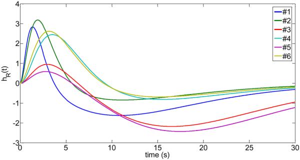
Computed respiratory response functions parameterized by where where for subjects #1 to #6 using the algorithm from Fig.1.
Fig.6.

Comparison of the respiratory response functions from this research with previous published work (Birn et. al. (2008)). The solid blue line is the mean over all subjects, and the broken lines are the upper and lower limit of one standard deviation from the mean of all subjects.
Accuracy of the optimization method to determine physiological response functions from limited data
The low-frequency physiological response functions were determined with high accuracy using all available data for each subject. Using 10 data sets for estimation of the unknown parameters and another 10 data sets for validation (determination of the optimum curvature), and each data set consisted of 200 time frames, this amounted to 4000 data points to determine the hemodynamic response functions for each subject. It is important to investigate how practical the proposed optimization techniques is to estimate the physiological response functions based on limited data such as a single resting-state data set for estimation of the parameters and another independent resting-state data set for validation. In Fig.7 and corresponding Table 4 we show as an example the results for the cardiac response function of subject #1. As can be seen, the cardiac response function can be determined quite accurately based on 2 independently collected data sets. Specifically, we used the following 3 scenarios to determine the cardiac response function for subject #1: Low TR data sets (TR 700ms for estimation, TR 800ms for validation), intermediate TR data sets (TR 1600ms for estimation, TR 1700ms for validation), and long TR data sets (TR 2500ms for estimation, TR 2600ms for validation). Of particular importance is the computed mean squared error (MSE) of the obtained functions (based on 2 data sets) and the exact function according to Table 2 and Fig. 3 for subject #1.
Fig.7.
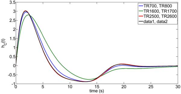
Reliability of the proposed optimization method to determine the cardiac response functions hc(t) of subject #1 using limited data (i.e. a single data set for estimation and a single data set for validation). The determined cardiac response functions are shown for the following four scenarios: 1. Blue curve: TR 700ms data set was used for estimation, TR 800ms data set was used for validation. 2. Green curve: TR 1600ms data set was used for estimation, TR 1700ms data set was used for validation. 3. Red curve: TR 2500ms data set was used for estimation, TR 2600ms data set was used for validation. 4. Black curve: Comparison to the full run using all data, i.e. TRs {700, 900, 1100, 1300, 1500, 1700, 1900, 2100, 2300, 2500} ms data sets were used for estimation, {800, 1000, 1200, 1400, 1600, 1800, 2000, 2200, 2400, 2600} ms data sets were used for validation).
Table 4.
Reliability of the proposed optimization method using a single data set
| data set used for estimation | data set used for validation | μ | a1 | a2 | a3 | a4 | a5 | a6 | α | MSE |
|---|---|---|---|---|---|---|---|---|---|---|
| TR 700 | TR 800 | 6.1 | 0.0934 | 2.0061 | 3.0154 | 0.0546 | 13.9663 | 16.2603 | 21.2708 | 0.010 |
| TR 1600 | TR 1700 | 4.8 | 0.0776 | 2.0115 | 3.5521 | 0.0427 | 14.8203 | 16.0985 | 20.0637 | 0.134 |
| TR 2500 | TR 2600 | 7.2 | 0.0977 | 2.0252 | 2.7860 | 0.0588 | 13.4378 | 16.4564 | 22.1770 | 0.0004 |
| data1 | data2 | 7.0 | 0.0984 | 2.0208 | 2.8143 | 0.0584 | 13.4949 | 16.2035 | 21.8294 | 0 |
Note: Rows 1 to 3 list the estimated parameters {a1 a2, a3, a4, a5, a6, α} of the cardiac response function for subject #1 from a single data set for estimation (see first column) and another single data set for validation (see second column). The last row contains the parameters for the full run using datal and data2 (see Fig.1, Table 2). The third column lists the optimum curvature where the minimum of the objective function occurred using the validation data set. The final column list the mean-squared error (MSE) of each estimated cardiac response function to the optimized cardiac response function using all available fMRI data as listed for subject #1 in the last row and Table 2.
Explained variance by physiological waveforms
For all brain fMRI data (all TR data sets and all subjects combined), we calculated the cumulative distribution of the residual variance by modeling all four (low-and-high-frequency) physiological regressors optimized at each voxel time series and computed the probability distribution p(V > ν) where V is the random variable representing the explained variance by all physiological noise sources combined. As is shown in Fig.8, to obtain a value of 10% or larger for the explained variance by all physiological noise sources, only 24% of all brain voxels are affected. However, this number increases to 64% of all voxels for an explained variance of 5% or larger.
Fig.8.
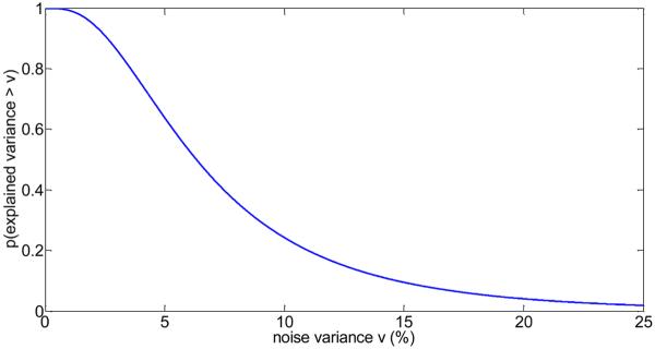
Probability of a brain voxel to have a physiological noise variance larger than v (in %), considering the combination of all four physiological noise sources. For example, the probability to obtain an explained noise variance of at least 10% is about 0.24, and the probability to obtain an explained noise variance of at least 5% is about 0.64.
To calculate accurate p-values of the explained variance, it is necessary to obtain a realistic null distribution of the voxel time series that does not contain any of the physiological noise characteristics and perform the same type of analysis (optimizing the temporal shift of the high-frequency regressors) on the null data with the voxel-optimized design matrix X. However, to eliminate physiological noise is not possible in a living subject. We proceeded by using wavelet-resampling techniques (Breakspear et. al., 2004; Bullmore et. al., 2001) to randomize the voxel time courses without affecting the inherent autocorrelation in the data and computed the null distribution of the explained variance. For specific p-values (p=0.05, p=0.01, p=0.001) of the explained variance, we calculated for each subject the variance contribution of each physiological waveform (Xi) and all physiological waveforms (X1X2X3X4) combined (see Table 5). Furthermore, we repeated the analysis using the previously published low-frequency physiological response functions of Chang et. al. (2009) and Birn et. al. (2008). As can be seen in Table 5, our approach yielded increased values of the explained variance (for example at p=0.001, 18% explained variance by our method versus 17.9% explained variance using the previously published waveforms). To compare above results with data that were not smoothed in the pre-processing stage, we repeated the analysis and computed the explained variance by all physiological regressors (Table 6). For all subjects, we obtained that the high-frequency regressors were able to explain more variance whereas the low-frequency regressors yielded a decrease of the explained variance. Overall, the combined effect of all 4 physiological regressors on using unsmoothed data was a reduction of explained variance for all subjects (compare Table 5 and Table 6).
Table 5.
Mean explained variance by physiological noise at different p values for smoothed data
| p | X1 (%) HF cardiac | X2 (%) HF resp | X3 (%) LF cardiac | X4 (%) LF resp | [X1 X2 X3 X4] (%) | Affected voxels (%) |
|---|---|---|---|---|---|---|
| 0.05 | 1.3+0.3 | 3.1±0.7 | 2.0±0.7 | 2.2±0.5 | 11.2±1.1 | 34.5±10.4 |
| (0.05) | (1.3±0.3) | (3.3±0.7) | (1.9±0.7) | (1.9±0.4) | (11.1 ±1.4) | (30.2±11.4) |
| 0.01 | 1.3±0.4 | 3.8±1.0 | 2.5±1.0 | 2.7±0.7 | 14.1+1.5 | 11.8+6.5 |
| (0.01) | (1.4±0.4) | (4.3±1.0) | (2.3±1.1) | (2.3±0.7) | (14.0±1.9) | (9.9±6.2) |
| 0.001 | 1.6±0.7 | 4.8±1.6 | 3.4±1.6 | 3.4±1.2 | 18.0±2.2 | 3.5±3.1 |
| (0.001) | (1.7±0.6) | (5.6±1.8) | (3.0±2.0) | (2.9±1.0) | (17.9±2.5) | (2.9±2.4) |
Note: The columns refer to the type of physiological noise averaged over all subjects (X1: high-frequency cardiac waveform, X2: high-frequency respiratory waveform, X3: low-frequency cardiac waveform, X4: low-frequency respiratory waveform). The rows refer to different p values (uncorrected). The numbers without parenthesis refer to the optimized model using the low-frequency waveforms in this research, whereas the numbers in parenthesis refer to the low-frequency model of Chang et. al. (2009) and Birn et. al. (2008). The last column refers to the percentage of the voxels that are affected by all 4 regressors.
Table 6.
Mean explained variance by physiological noise at different p values for unsmoothed data
| p | X1 (%) HF cardiac | X2 (%) HF resp | X3 (%) LF cardiac | X4 (%) LF resp | [X1 X2 X3 X4] (%) | Affected voxels (%) |
|---|---|---|---|---|---|---|
| 0.05 | 1.5±0.2 | 3.2±0.9 | 1.4±0.3 | 1.3±0.2 | 9.8±0.9 | 20.3±8.7 |
| (0.05) | (1.5±0.2) | (3.3±0.8) | (1.2±0.3) | (1.2±0.2) | (9.6±0.8) | (19.7±8.7) |
| 0.01 | 1.7±0.3 | 4.3±1.3 | 1.7±0.6 | 1.6±0.4 | 12.5±1.0 | 7.3±4.6 |
| (0.01) | (1.8±0.3) | (4.6±1.3) | (1.4±0.5) | (1.5±0.4) | (12.3±0.9) | (7.1 ±4.6) |
| 0.001 | 2.3±0.6 | 6.0±2.1 | 2.2±0.9 | 1.9±0.7 | 16.2±1.4 | 2.2±1.9 |
| (0.001) | (2.3±0.5) | (6.5±2.1) | (1.7±0.8) | (1.7±0.7) | (15.9±1.0) | (2.2±1.9) |
Note: The columns refer to the type of physiological noise averaged over all subjects (X1. high-frequency cardiac waveform, X2: high-frequency respiratory waveform, X3: low-frequency cardiac waveform, X4: low-frequency respiratory waveform). The rows refer to different p values (uncorrected). The numbers without parenthesis refer to the optimized model using the low-frequency waveforms in this research, whereas the numbers in parenthesis refer to the low-frequency model of Chang et. al. (2009) and Bim et. al. (2008). The last column refers to the percentage of the voxels that are affected by all 4 regressors.
In Fig.9(a–f) we show the locations of voxels that are affected by the high-frequency cardiac (X1) and respiratory (X2) waveforms, and the low-frequency cardiac (X3) and respiratory (X4) waveforms. It is very clear that X1 (first row in Fig.9(a–f)) affects mainly the brainstem region and the major blood vessels. Voxels in the prefrontal region are not affected. The brain locations have a sparse appearance, and the number of voxels affected can vary significantly among all subjects. For example, subjects #2 and #5 show a very small number of voxels affected at the p<0.01 level (yellow and white color). The influence of the high-frequency respiratory wave function X2) can be quite strong for certain subjects (#1,#3,#5,#6) and show many distinct locations throughout the brain, such as prefrontal cortex, cerebellum, brainstem, temporal lobe, midbrain and occipital cortex (second row in Fig.9(a–f)). Only for subjects #2 and #4 the affected regions are mostly cerebellum and visual cortex. Less cardiac activity does not imply less respiratory activity as subject #5 clearly shows. Here, the respiratory activity is very large compared to the cardiac activity.
Fig.9.


abc. Subject #1,#2,#3. Locations of significant voxels associated with high-frequency cardiac activity (1. row), high-frequency respiratory activity (2. row), low-frequency cardiac activity (3. row), low-frequency respiratory activity (4. row). The meaning of the color scale is: p=0.05 (red), p=0.01 (yellow), p=0.001 (white). The white dot visible in the structural images for the center slices is a vitamin D capsule (attached to the forehead) to indicate the right side.
def. Subject #4,#5,#6. Locations of significant voxels associated with high-frequency cardiac activity (1. row), high-frequency respiratory activity (2. row), low-frequency cardiac activity (3. row), low-frequency respiratory activity (4. row). The meaning of the color scale is: p=0.05 (red), p=0.01 (yellow), p=0.001 (white). The white dot visible in the structural images for the center slices is a vitamin D capsule (attached to the forehead) to indicate the right side.
The voxels affected by the low-frequency cardiac waveform (third row in Fig.9(a–f)) are concentrated at the region near the top portion of the cerebellum and the lower visual cortex as well as some focal regions in the medial prefrontal cortex. For all subjects except #6, the affected voxels show a sparse location. Subject #6, however, shows a large influence of low-frequency cardiac activity in visual cortex and prefrontal cortex. The low-frequency respiratory waveform (fourth row in Fig.9(a–f)) has several regions in common with the low-frequency cardiac waveform (visual cortex, lingual cortex, temporal cortex, prefrontal cortex) (subjects #1,#2,#4,#6). For subjects #3 and#5, the low-frequency respiratory contributions are minor compared with the other subjects.
We also calculated highly significant clusters of physiological noise activity for a family-wise error rate FWE<0.05, as determined by AlphaSim in AFNI (Cox, 1996) using an individual p-value=0.001 with cluster size of at least 240mm3. For the high-frequency cardiac waveform, all significant clusters were at the brainstem and larger blood vessels, and no cortical area was involved. For the high-frequency respiratory waveform, significant clusters were found in fusiform gyrus (subjects #1,#5,#6), lingual gyrus (subjects #1,#5) and cerebellum (subjects #1,#5,#6). The low-frequency cardiac waveform had significant clusters in caudate nucleus (subject #1), cerebellum (subjects #1,#2,#6), fusiform gyrus (subject #1), lingual gyrus (subjects #1,#2,#6), temporal cortex (subjects #1,#2,#6) and frontal cortex (subject #6). Significant clusters for the low-frequency respiratory waveform were found in calcarine cortex (subject #1), cerebellum (subjects #1,#6), lingual gyrus (subject #1), temporal cortex (subject #6) and frontal cortex (subject #6).
Aliasing of high-frequency physiological waveforms as a function of TR
To show the effect of aliasing of the high-frequency cardiac rate, we parameterized the cardiac waveform of each subject by a Gaussian distribution with mean and standard deviation given in Table 1 and calculated the aliased frequency distribution after sampling by different using Eq.(5). Fig.10 shows the distribution of the high-frequency cardiac waveform of subject #6 and Fig.11 the corresponding aliased frequency spectrum after sampling with TR = 2s. Please note that Fig.10 is a hypothetical cardiac waveform of subject #6, based on the Gaussian distribution and the mean and standard deviation values of subject 6. For better visibility of the effect of aliasing we have colored different frequency bands of the cardiac rate in Fig.10 and show explicitly in Fig.11 where each of the colored frequency bands aliases to. For example, the frequencies near 1Hz of the peak region in Fig.10 (red color) alias at TR = 2s to the low-frequency range near 0Hz, whereas the frequency regions one standard deviation away from the peak in Fig.10 (turquois blue colors) alias to the frequency-range larger than 0.1Hz.
Fig.10.

Approximate frequency spectrum of a typical high-frequency cardiac waveform with mean frequency 0.98Hz and standard deviation 0.067Hz. The coloring emphasizes different frequency bands and the labels L and R refer to the left (L) or right (R) side of the distribution (compare with Fig.11).
Fig.11.

Aliased frequency spectrum of the high-frequency cardiac waveform from Fig.10 using a sampling time TR = 2s. The coloring of the aliased frequencies corresponds to the coloring of the un-aliased frequencies in Fig.10. The labels L and R refer to the left (L) or right (R) side of the distribution in Fig. 10. The black curve is the total probability density of the aliased frequencies.
Next, we calculated the probability that the distribution of the high-frequency cardiac waveform after sampling at a TR will be larger than 0.1Hz. Fig.12 shows the results of the probability p(f > 0.1Hz) for all subjects and TRs from 0 to 4s. As can be seen, there exist distinctive plateaus where p(f > 0.1Hz) is maximum. For example, subject #6 with a cardiac rate of 0.98Hz (σ = 0.067Hz) has p(f > 0.1Hz) ≈ 1 for TR < 0.8s and 1.3s < TR < 1.7s. Also, in the vicinity of TR = 2.5Hz the value for p(f > 0.1Hz) has a maximum. In general, those TRs for which p(f > 0.1Hz) is maximum (or close to maximum) offer advantages in terms of separating the cardiac influence on brain voxel time series associated with the high-frequency cardiac waveform from the low-frequency BOLD response, which is usually related to the frequency range f < 0.1Hz because of the low-pass functional form of the hemodynamic response function. If this is the case, the cardiac noise that aliases to the f > 0.1Hz range does not contaminate the BOLD frequency range and can be eliminated by digital low-pass filtering, providing voxel time-series with less variance from cardiac noise.
Fig.12.
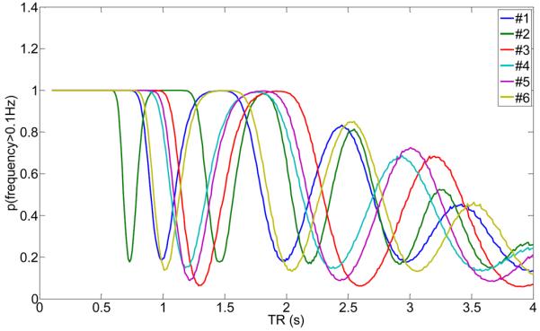
Probability that the frequency of the cardiac waveform after sampling at the given TR is above 0.1Hz for subjects #1 to #6 using the information from Table 1. The higher the probability, the less likely it will be that the cardiac frequency occupies the low-frequency spectrum of the BOLD response.
Please note that the optimum TRs (when p(f > 0.1Hz) ≈ 1) is different for each subject since the subjects had mean heart rates between 0.77Hz and 1.37Hz. However, each subject had a stable heart rate over a scanning time of 2h with a small variance (compare Table 1). Thus, choosing a more optimal TR with less interference from cardiac noise is possible, especially if the study in question focuses on problematic areas that are known to vibrate with the cardiac rate, for example the brainstem.
As the TR can be optimal, it can also be detrimental to the data. For example, if a standard TR = 2s would have been chosen for subject 6, the value for p(f > 0.1Hz) is very low (<0.2), and all the high-frequency cardiac noise will alias into the f < 0.1Hz BOLD range.
For the high-frequency respiratory waveform, the aliasing behavior at typical TRs is very different (Fig.13). Because of its lower mean frequency values (see Table 1), aliasing of the respiratory rate for TR < 2.5s will be very small leading to large values of p(f > 0.1Hz) at typical TRs. Thus, there is no preference of certain TRs as long as TRs are chosen to be less than 2.5s.
Fig.13.

Probability that the frequency of the respiratory waveform after sampling at the given TR is above 0.1Hz for subjects #1 to #6 using the information from Table 1. The higher the probability, the less likely it will be that the respiratory rate occupies the low-frequency spectrum of the BOLD response.
So far we considered only the high-frequency waveforms for the cardiac rate and the respiratory rate. The low-frequency waveforms for both physiological noise sources are less than 0.1Hz and will not be affected by aliasing at typical TRs used in fMRI. Thus, in order to eliminate these low-frequency noise sources, digital low-pass filtering will not be possible. Only modeling will work, as we have shown here in the first part of this research.
Validation
So far we have assumed that the probability density function of the physiological noise sources is stationary for each subject during the entire fMRI scanning time of 2h. This is a very strong assumption which needs validation. In the following we show that these assumptions are approximately true for the cardiac waveform using the collected pulse-oximeter data of all subjects by computing empirical results corresponding to the theoretical figures 10–12. In Fig.14 (top) we show the cardiac frequency as a function of time for subject #6, as computed for one pulse-oximeter data set that was simultaneously recorded with the fMRI (TR 700ms data) for this subject. Using kernel density estimation (Silverman, 1986), we computed the probability density function of the cardiac frequency (Fig.14 (middle)), which shows a maximum near 1Hz and rapid fall-off for higher and lower frequencies. Using this empirically determined probability density function, we calculated the aliased frequency spectrum for a sampling rate Δt = 2s (using Eq.(2)) and determined the probability p(f > 0.1Hz) by integrating all frequencies larger than 0.1Hz (see Fig.14 (bottom)). Next, to prove that the frequency probability density function is also quasi-stationary across the entire 2h scanning time, we calculated the empirical mean probability and its standard deviation for all 20 pulse-oximeter data sets for each subject (which were collected over a 2h time period while the subject was being scanned for fMRI), based on the frequency probability density functions that were estimated from all corresponding pulse-oximeter raw data. Results are shown in Fig.15 for all subjects.
Fig.14.

Subject #6: Instantaneous frequency as a function of time based on the pulse-oximeter measurements (top), corresponding probability density function of the frequencies (middle), and calculated aliasing probability that the pulse-oximeter frequencies after sampling at the given TR are above 0.1 Hz.
Fig.15.

Solid (center) line: Calculated mean aliasing probability that the pulse-oximeter frequencies after sampling at the given TR are above 0.1 Hz for each subject. The mean was calculated using all 20 different pulse-oximeter data for each subject collected within a 2 hour scanning time. Broken lines (above and below center line): One standard deviation above and below the corresponding mean probability.
Temporal SNR
To compute the temporal SNR of our fMRI data, we have bandpass-filtered all raw fMRI data to remove low-frequency drift less than 0.01Hz and removed all frequencies larger than 0.1Hz to capture the dominant frequency region of the BOLD response. Fig.16 shows the temporal SNR for all fMRI data (subjects #1 to #6) as a function of TR. Due to aliasing of the high-frequency cardiac rate, we get more or less aliasing into the low-frequency range (f < 0.1Hz), resulting in smaller or higher temporal SNR, depending on the TR used. All subjects show an oscillatory behavior of the temporal SNR, similar to the curves in Fig.12. From theory, there should be a high correlation of the probability that the cardiac waveform after sampling is above 0.1Hz and the temporal SNR restricted to a frequency range less than 0.1Hz. This is indeed the case for the majority of all subjects, as shown in Table 7. In fact, for subjects #1,#3,#4,#6, the correlation coefficient between the equivalent curves of Fig.12 and Fig.16 is at least 0.24. For subject #3 the correlation coefficient is very high (0.65). Only for subject #2 and #5, the correlation coefficient is lower (−0.27 for #2 and −0.01 for #5), which was expected because of the small number of voxels affected by the high-frequency cardiac waveform, as shown in Fig.9e for subject #5 (top row). It is interesting to observe that the minima and maxima predicted by the aliasing analysis of the high-frequency cardiac noise (Fig.12) indeed correspond well to the minima and maxima of the temporal SNR of Fig.16.
Fig.16.
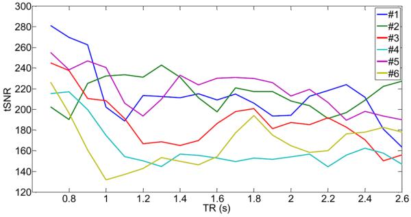
Calculated temporal SNR (tSNR) for all voxels that show a cardiac activity with p<0.05, as a function of TR for all six subjects. All fMRI data were band-pass filtered using the frequency range [0.01,0.1]Hz. Note the cyclic behavior of the curves similar to the ones in Fig.12.
Table 7.
Correlation coefficient of p(f > 0.1Hz) of the cardiac waveform (from Fig.12) with the tSNR of fMRI data (from Fig.16).
| cc | |
|---|---|
| Subject #1 | 0.33 |
| Subject #2 | −0.27 |
| Subject #3 | 0.65 |
| Subject #4 | 0.44 |
| Subject #5 | −0.01 |
| Subject #6 | 0.24 |
| mean | 0.23 |
Comparison with RETROICOR on temporal SNR
To determine the effectiveness of our method with an established method, we used RETROICOR (Glover et. al., 2000). RETROICOR models the high-frequency physiological noise components by a low-order Fourier series that are expanded in terms of phases, which can be derived from external measurements. We used a Fourier series of order 2 for both cardiac and respiratory noise components, leading to 4 cardiac (2 sine functions, 2 cosine functions) and 4 respiratory regressors (2 sine functions, 2 cosine functions). After preprocessing with RETROICOR, we calculated the temporal SNR for voxels that have high-cardiac content. We also repeated the analysis using our proposed correction method for the high-frequency waveforms using CHF(t) and RHF(t) as regressors. Results are shown in Fig.17. Here, the top graph shows that the temporal SNR is increased by about 10 units (on average) at specific TRs when RETROICOR is used in the preprocessing stage. For example, the temporal SNR of subject #1 is increased by about 15–18 units for the TR- interval [0.9s,1.2s] when the high-frequency cardiac noise aliases mostly into the f < 0.1Hz frequency range (see Fig.15 top left). For other subjects, similar scenarios can be found. When our method is used, we obtain also an increase of 10 units (on average) of the temporal SNR. It is shown in Fig.17 (middle graph), that RETROICOR and our method are comparable in eliminating cardiac noise contributions in fMRI data. However, small differences (|Δ tSNR| < 4) exist for several TR- intervals. For example, the temporal SNR of subject #3 for the TR- interval [1.1s,1.3s] (where the high-frequency cardiac noise aliases mostly into the f < 0.1Hz frequency range according to Fig.15) is improved by our method.
Fig.17.

Comparison of performance between our method and RETROICOR for all voxels that show a cardiac activity with p<0.05, as a function of TR for all six subjects. Top: Difference in temporal SNR (tSNR) for RETROICOR-corrected data and uncorrected data (from Fig.16), after bandpass-filtering using the frequency range [0.01,0.1]Hz. Middle: Difference in temporal SNR for data corrected by the proposed method (using the high-frequency cardiac and respiratory functions) and by RETROICOR, after bandpass-filtering using the frequency range [0.01,0.1]Hz. Bottom: Difference in the adjusted R2 statistic for data corrected by the proposed method (using the high-frequency cardiac and respiratory functions) and by RETROICOR.
For simplicity, in the previous comparison we have not taken into account the different number of regressors for our method and RETROICOR. From a statistical perspective, a simpler model is usually preferred over a more complex model (if all other parameters or features are equal). Thus, to assess the model fit of each method accurately and explicitly take into account the different numbers of regressors in the design matrix (2 for our method versus 8 for RETROICOR), we computed for both methods the adjusted R2 statistic (see for example Montgomery and Runger (2003)). In Fig.17 (bottom graph) we show the difference in the adjusted R2 statistic between our method and RETROICOR. This graph shows that the difference of the adjusted R2 statistic is small and satisfies which implies that our method and RETROICOR have similar performance, since the average value is about 0.03.
DISCUSSION
The purpose of this research was to simultaneously estimate the physiological noise contributions arising from cardiac and respiratory activity in fMRI resting-state data by using physiological data acquired with pulse-oximeter and respiratory belt, and investigate the aliasing properties of the high-frequency cardiac noise as a function of TR. We have explicitly modeled the physiological noise by four different regressors. The first two regressors represented the high-frequency cardiac and respiratory activity. These functions were obtained from the physiological measurements and phase-optimized for each voxel to obtain the best time-shift of the regressors to accommodate the timing difference between the measured physiological waves at fingertip or abdomen and the different locations of cerebral tissue. Besides modeling of the high-frequency physiological noise sources, we have calculated the low-frequency changes of the cardiac and respiratory noise sources and computed a cardiac and a respiratory hemodynamic response function, optimized for each subject.
Optimization algorithm and cross-validation
A strength of this research is that the computed physiological hemodynamic response functions were not derived from specific voxels using a convolution approach but instead from an optimization algorithm with cross-validation using a parameterization of the cardiac and respiratory response functions with forms previously established (see Chang et. al. (2009) and Birn et. al.(2008)). We explicitly added a first-order derivative and applied constraints to allow for subject-specific variations of the hemodynamic response. With this subject-specific approach, low-frequency physiological response functions were obtained. We found that the off-diagonal elements of the covariance matrix of the four physiological regressors were not larger than 0.15 for variance normalized regressors, indicating a small overlap of the noise sources. Similar to the approach suggested by Chang et. al. (2009), we used the standard deviation using a sliding time-window approach to determine the low-frequency respiratory waveform related to differences in the breathing inspiration rate instead of the approach used by Birn et. al. (2008).
The methods proposed in this research are accurate, even if only a single fMRI resting-state data set is used for estimation and another fMRI resting-state data set is used for validation. We attribute the accuracy of the proposed method to the cross-validation step in combination with penalizing curvature. We obtained characteristic minima spanning a range of about 2 units in curvature in the cross-validation step leading to accurate prediction of the physiological response functions, as shown explicitly for the cardiac response function of one subject (#1). Even if different data sets are used, the corresponding physiological response functions are similar.
The results obtained can also be slightly improved, if desired, by using both data sets for estimation and validation (i.e. using set1 for estimation, set2 for validation getting hc(t), then using set2 for estimation, set1 for validation getting ), and then calculating the average of the obtained response functions (i.e. )). Switching estimation and validation steps will result in maximum efficiency to solve the optimization and validation problem.
Nonparametric estimation of p-values
To arrive at accurate p-values of the explained variances by the physiological regressors, we used wavelet-resampling of the fMRI resting-state data to obtain approximate null data, and applied the same type of methodology that we used for modeling of the physiological noise sources to the null data. We found this step to be important to correct for the optimized time-shift selection at each voxel to obtain the high-frequency cardiac and noise regressors.
Comparison of the physiological response functions with other studies
The subject-specific physiological response functions obtained show some differences to the types proposed by Chang et. al. (2009) and Birn et. al. (2008). For example, with our approach we obtained cardiac response functions that have a first maximum between 1.5s and 5s and minimum between 11s and 14s. Furthermore, for one subject (#1) we obtained a pronounced second maximum at about 19s which arises by the inclusion of the derivative term. A second maximum was also found by Chang et. al. (2009) but not explicitly modeled. A more recent approach (Falahpour et. al. (2013)) also showed a first maximum at about 4s, a minimum at 10s and a second maximum at about 18s, similar to our results. For all subjects we found that the inclusion of the derivative term in the model is necessary to determine the optimum cardiac response function. To obtain a subject optimized respiratory response function, we found that the solution of the optimization problem can be parameterized by the form given by Birn et. al. (2008), but with different coefficients. There is no need for inclusion of a derivative term to obtain an optimum respiratory response function. Besides magnitude differences, we found that the occurrence of the undershoot is subject-specific and can occur between 4s and 9s. However, using subject-specific physiological response functions leads only to a small increase of the explained noise variance. In the study by Falahpour et. al. (2013) there was small improvement in the average explained variance (similar to our results), but it was shown that using the subject-specific filters expands the explained variance in the entire brain.
We found that the difference in the respiratory wave forms using the method by Chang et. al. (2009) versus the method by Birn et. al. (2008) is rather minor, since both functions are highly correlated with correlation coefficient larger than 0.7, according to our research.
Effect of spatial smoothing versus no smoothing
Spatial filtering is a common preprocessing technique that is used to increase the signal- to-noise ratio in fMRI data. Since high-frequency information is reduced by spatial filtering, it is conceivable that high-frequency physiological noise regressors will be less effective in smoothed data and may reduce the data correction. On the other hand, low-frequency effects caused by the low-frequency cardiac and respiratory hemodynamic response functions may show the opposite effects and lead to less data correction for unsmoothed data. Our analysis comparing the variance explained for smoothed versus unsmoothed data showed that by using all four noise regressors simultaneously, the data correction of all 6 subjects for smoothed data is still better than for unsmoothed data, due to a larger effect of the low-frequency physiological response functions on the data correction.
Appearance of activation maps
The subject-specific noise activity maps obtained have a sparse appearance and show that the physiological noise attributed to all four low-and high-frequency waveforms is more voxel-specific rather than affecting larger continuous regions of the brain. For example, the high-frequency cardiac waveform mostly affected the brainstem and larger blood vessels in the lower slices rather than the entire brain. Upper slices showed a very small amount of high-frequency cardiac noise, and it appears that most of grey matter and brain periphery were not affected.
Existence of subject-specific optimal TRs
A particular focus of this research was to investigate if a subject-optimized TR can be chosen where the high-frequency cardiac rate does not alias into the low-frequency BOLD range. This is indeed the case as we have shown by computing the temporal SNR as a function of TR. Since the cardiac high-frequency activity was very stable for each subject during a 2h of scanning time, it is possible to predict where the cardiac frequency will alias to. Even if the empirical probability density functions of the cardiac rate are computed from the pulse-oximeter data and the obtained density differs from an ideal Gaussian distribution, the variance of the density is still small enough so that aliasing after digital sampling is predictable and the empirical findings shown in Fig.15 agree well with the theoretical predictions from Fig.12. Thus, by knowing the mean cardiac frequency and its standard deviation of each subject (for example from pilot studies), it is possible to choose an optimal TR to reduce aliasing of the high-frequency cardiac noise into the low-frequency BOLD range. This approach could have advantages for mapping activations of the brainstem or nearby spinal cord regions, which are inherently difficult to study with fMRI because of the large vibration associated with the heartbeat. As we have shown, the temporal SNR can be improved by about 40–50 in problem areas if an optimal TR is chosen. However, for the majority of grey matter voxels in the upper cortex, high-frequency cardiac noise is relatively absent.
The results obtained in this research have been obtained for 2h of resting-state data collection with 6 young healthy volunteers who had previous fMRI scanning experience. None of the subjects were recruited because of prior measurements of the heart rate. Furthermore, none of the subjects were selected based on a low variance of heart rate fluctuations. Thus, the subjects scanned were a true random sample of young students with prior fMRI experience. For activation data (instead of resting-state data), however, the method of finding an optimal TR may be less useful (depending on the task), because in activation data a larger variance of the heart rate fluctuations has been observed leading to less structured aliasing properties (Lund et al, 2006).
Limitations of this study
A limitation of this study is that only partial coverage of the brain was obtained, due to the short TRs used. Physiological noise affects have been shown in widespread regions of the brain (see for example Chang et. al., 2009). Thus, it would be more desirable to have full brain coverage and investigate the effects of the proposed approach in the entire brain. Although pulsation effects are higher in the lower brain regions (which we focused on in this study), the proposed methods may have been more effective in the lower brain regions. Also, amplitude changes of the pulsations due to vasomotion were neglected by normalizing the amplitude of the high frequency cardiac wave to one.
A computational limitation of this study is that the parameters of the cardiac and respiratory low-frequency hemodynamic response functions were determined independently. It is conceivable that a simultaneous estimation of both functions may have advantages and may be more accurate because other research have shown that there are extensive regions of grey matter which are affected by both cardiac and respiration-related fluctuations (see for example Chang et. al. (2009)). However, due to the large increase of local minima in the solution space going from 6 to 12 dimensions, finding a global constraint solution in a 12-dimensional space is considerably more challenging and beyond the aims of this research project.
Finally, we provided only a limited comparison with another established method (RETROICOR) to model the high-frequency cardiac and respiratory noise sources. Preliminary results indicate a similar performance between our method and RETROICOR, based on the increase of the temporal SNR and assessment of the model fit using the adjusted R2 statistic. A more complete study of the differences, similarities and effectiveness of RETROICOR and our proposed method is beyond the scope of this research project.
CONCLUSIONS
In summary, modeling of all four physiological noise sources can lead to significant improvements in fMRI resting-state data quality. The high-frequency cardiac noise is mostly associated with the brainstem, nearby spinal cord and larger blood vessels. The cardiac noise affecting the brainstem and other nearby regions can be efficiently eliminated for fMRI using imaging at subject-specific TRs where the high-frequency cardiac noise will not alias into the BOLD frequency range.
ACKNOWLEDGMENTS
This research was partially supported by the NIH (grant number 1R01EB014284).
APPENDIX
In the following, we derive the Fourier transform of a sampled continuous time-dependent function f(t), as used in Eq.(2). Sampling f(t) at discrete intervals ΔT yields the sampled function, , given by
| (A1) |
where
| (A2) |
is the sampling function and
| (A3) |
is the Dirac delta function. Since the sampling function is periodic, it can be expanded in a Fourier series according to
| (A4) |
where the Fourier coefficients, cn, are calculated by
Thus,
| (A5) |
The Fourier transform of the sampling function, S(μ), where μ indicates the frequency variable, is obtained by using (A2–A5). We obtain:
| (A6) |
Now, let F(μ) be the Fourier transform of f(μ). Furthermore, let the letter indicate the Fourier transform operator and the symbol * to note convolution. Then, the Fourier transform of , , becomes using (A1) and (A6):
and the proof of Eq.(2) is complete.
Footnotes
Publisher's Disclaimer: This is a PDF file of an unedited manuscript that has been accepted for publication. As a service to our customers we are providing this early version of the manuscript. The manuscript will undergo copyediting, typesetting, and review of the resulting proof before it is published in its final citable form. Please note that during the production process errors may be discovered which could affect the content, and all legal disclaimers that apply to the journal pertain.
REFERENCES
- Beall EB, Lowe MJ. Isolating physiologic noise sources with independently determined spatial measures. NeuroImage. 2007;37(4):1286–300. doi: 10.1016/j.neuroimage.2007.07.004. [DOI] [PubMed] [Google Scholar]
- Beall EB, Lowe MJ. The non-separability of physiological noise in functional connectivity MRI with spatial ICA at 3T. J. Neuroscience Methods. 2010;191:263–276. doi: 10.1016/j.jneumeth.2010.06.024. [DOI] [PubMed] [Google Scholar]
- Beall EB. Adaptive cyclic physiological noise modeling and correction in functional MRI. J. Neuroscience Methods. 2010;187:216–228. doi: 10.1016/j.jneumeth.2010.01.013. [DOI] [PubMed] [Google Scholar]
- Beckmann CF, DeLuca M, Devlin JT, Smith SM. Investigations into resting-state connectivity using independent component analysis. Philos. Trans. R. Soc. Lond., B Biol. Sci. 2005;360:1001–1013. doi: 10.1098/rstb.2005.1634. [DOI] [PMC free article] [PubMed] [Google Scholar]
- Bhattacharyya PK, Lowe MJ. Cardiac-induced physiologic noise in tissue is a direct observation of cardiac-induced fluctuations. Magn Reson Imag. 2004;22:9–13. doi: 10.1016/j.mri.2003.08.003. [DOI] [PubMed] [Google Scholar]
- Birn MB, Smith MA, Jones TB, Bendettini PA. The respiration response function: The temporal dynamics of fMRI signal fluctuations related to changes in respiration. NeuroImage. 2008;40:644–654. doi: 10.1016/j.neuroimage.2007.11.059. [DOI] [PMC free article] [PubMed] [Google Scholar]
- Biswal B, DeYoe AE, Hyde JS. Reduction of physiological fluctuations in fMRI using digital filters. Magn Reson Med. 1996;35:107–13. doi: 10.1002/mrm.1910350114. [DOI] [PubMed] [Google Scholar]
- Breakspear M, Brammer M, Bullmore E, Das P, Williams L. Spatiotemporal wavelet re-sampling for functional neuroimaging data. Hum Brain Mapp. 2004;23:1–25. doi: 10.1002/hbm.20045. [DOI] [PMC free article] [PubMed] [Google Scholar]
- Brooks JC, Beckmann CF, Miller KL, Wise RG, Porro CA, Tracey I, Jenkinson M. Physiological noise modeling for spinal functional magnetic resonance imaging studies. NeuroImage. 2008;39:680–92. doi: 10.1016/j.neuroimage.2007.09.018. [DOI] [PubMed] [Google Scholar]
- Bullmore E, Long C, Suckling J, Fadili J, Calvert G, Zelaya F, Carpenter T, Brammer M. Colored noise and computational inference in neurophysiological (fMRI) time series analysis: Resampling methods in time and wavelet domains. Hum Brain Mapp. 2001;12:61–78. doi: 10.1002/1097-0193(200102)12:2<61::AID-HBM1004>3.0.CO;2-W. [DOI] [PMC free article] [PubMed] [Google Scholar]
- Chang C, Glover GH. Effects of model-based physiological noise correlation on default mode network anti-correlations and correlations. NeuroImage. 2009;47:1448–1459. doi: 10.1016/j.neuroimage.2009.05.012. [DOI] [PMC free article] [PubMed] [Google Scholar]
- Chang C, Cunningham JP, Glover GH. Influence of heart rate on the BOLD signal: The cardiac response function. NeuroImage. 2009;44:857–869. doi: 10.1016/j.neuroimage.2008.09.029. [DOI] [PMC free article] [PubMed] [Google Scholar]
- Chuang KH, Chen JH. IMPACT: image-based physiological artifacts estimation and correction technique for functional MRI. Magn Reson Med. 2001;46:344–53. doi: 10.1002/mrm.1197. [DOI] [PubMed] [Google Scholar]
- Cordes D, Haughton VM, Arfanakis K, Carew JD, Turski PA, Moritz CH, Quigley A, Meyerand ME. Frequencies contributing to functional connectivity in the cerebral cortex in “resting-state” data. AJNR Am. J. Neuroradiol. 2001;22:1326–1333. [PMC free article] [PubMed] [Google Scholar]
- Cox RW. AFNI: software for analysis and visualization of functional magnetic resonance neuroimages. Comput. Biomed. Res. 1996;29:162–173. doi: 10.1006/cbmr.1996.0014. [DOI] [PubMed] [Google Scholar]
- Dagli MS, Ingeholm JE, Haxby JV. Localization of cardiac-induced signal change in fMRI. NeuroImage. 1999;9:407–15. doi: 10.1006/nimg.1998.0424. [DOI] [PubMed] [Google Scholar]
- Falahpour MF, Refai H, Bodurka J. Subject specific BOLD fMRI respiratory and cardiac response functions obtained from global signal. NeuroImage. 2013;72:252–264. doi: 10.1016/j.neuroimage.2013.01.050. [DOI] [PubMed] [Google Scholar]
- Gonzalez-Castillo J, Roopchansingh V, Bandettini PA, Bodurka J. Physiological noise effects on the flip angle selection in BOLD fMRI. NeuroImage. 2011;54:2764–2778. doi: 10.1016/j.neuroimage.2010.11.020. [DOI] [PMC free article] [PubMed] [Google Scholar]
- Glover GH, Lemieux SK, Drangova M, Pauly JM. Decomposition of Inflow and Blodd Oxygen Level-Dependent (BOLD) Effects with Dual-Echo Spiral Gradient-Recalled Echo (GRE) fMRI. Magn Reson Med. 1996;35:299–308. doi: 10.1002/mrm.1910350306. [DOI] [PubMed] [Google Scholar]
- Glover GH, Li TQ, Ress D. Image-based method for retrospective correction of physiological motion effects in fMRI: RETROICOR. Magn Reson Med. 2000;44:162–7. doi: 10.1002/1522-2594(200007)44:1<162::aid-mrm23>3.0.co;2-e. [DOI] [PubMed] [Google Scholar]
- Greve DN, Dale AM. Spatial noise cancellation for fMRI. NeuroImage. 2002;16:769–1198. [Google Scholar]
- Guijt M, Sluiter JK, Frings-Dresden MHW. Test-Retest Reliability of Heart Rate Variability and Respiration Rate at Rest and during light Physical Activity in Normal Subjects. Archives of Medical Research. 2007;38:113–120. doi: 10.1016/j.arcmed.2006.07.009. [DOI] [PubMed] [Google Scholar]
- Harvey AK, Pattinson KT, Brooks JC, Mayhew SD, Jenkinson M, Wise RG. Brainstem functional magnetic resonance imaging: disentangling signal from physiological noise. J Magn Reson Imag. 2008;28:1337–44. doi: 10.1002/jmri.21623. [DOI] [PubMed] [Google Scholar]
- Hu X, Le TH, Parrish T, Erhard P. Retrospective estimation and correction of physiological fluctuation in functional MRI. Magn Reson Med. 1995;34:201–12. doi: 10.1002/mrm.1910340211. [DOI] [PubMed] [Google Scholar]
- Kruger G, Kastrup A, Glover GH. Neuroimaging at 1.5T and 3.0T: Comparison of Oxygenation-Sensitive Magnetic Resonance Imaging. Magn Reson Med. 2001;45:595–604. doi: 10.1002/mrm.1081. [DOI] [PubMed] [Google Scholar]
- Kruger G, Glover GH. Physiological Noise in Oxygenation-Sensitive Magnetic Resonance Imaging. Magn Reson Med. 2001;46:631–637. doi: 10.1002/mrm.1240. [DOI] [PubMed] [Google Scholar]
- Le TH, Hu X. Retrospective Estimation and Correction of Physiological Artifacts in fMRI by Direct Extraction of Physiological Activity from MR Data. Magn Reson Med. 1996;35:290–298. doi: 10.1002/mrm.1910350305. [DOI] [PubMed] [Google Scholar]
- Lin F-H, Nummenmaa A, Witzel T, Polimeni JR, Zeffiro TA, Wang F-N, Belliveau JW. Physiological Noise Reduction Using Volumetric Functional Magnetic Resonance Inverse Imaging. Hum Brain Mapp. 2012;33(12):2815–2830. doi: 10.1002/hbm.21403. [DOI] [PMC free article] [PubMed] [Google Scholar]
- Lowe MJ, Mock BJ, Sorenson JA. Functional connectivity in single and multislice echoplanar imaging using resting-state fluctuations. NeuroImage. 1998;7:119–132. doi: 10.1006/nimg.1997.0315. [DOI] [PubMed] [Google Scholar]
- Lu H, Golay X, van Zijl PCM. Intervoxel Heterogeneity of Event-Related Functional Magnetic Resonance Imaging Responses as a Function of T1 Weighting. NeuroImage. 2002;17:943–955. [PubMed] [Google Scholar]
- Lund TE, Madsen KH, Sidaros K, Luo WL, Nichols TE. Non-white noise in fMRI: does modelling have an impact? NeuroImage. 2006;29:54–66. doi: 10.1016/j.neuroimage.2005.07.005. [DOI] [PubMed] [Google Scholar]
- Malik M. Heart Rate Variability. Circulation. 1996;93:1043–1065. [PubMed] [Google Scholar]
- Montgomery DC, Runger GC. Applied Statistics and Probability for Engineers. 3. Edition John Wiley and Sons; 2003. [Google Scholar]
- Murphy K, Birn RM, Handwerker DA, Jones TB, Bandettini PA. The impact of global signal regression on resting state correlations: Are anti-correlated networks introduced? NeuroImage. 2009;44:893–905. doi: 10.1016/j.neuroimage.2008.09.036. [DOI] [PMC free article] [PubMed] [Google Scholar]
- Nocedal J, Wright SJ. Numerical Optimization. Springer Series in Operations Research. 2006 [Google Scholar]
- Perlbarg V, Bellec P, Anton J-L, Pelegrini-Issac M, Doyon J, Benali H. CORSICA: correction of structured noise in fMRI by automatic identification of ICA components. Magn Reson Imag. 2007;25:35–46. doi: 10.1016/j.mri.2006.09.042. [DOI] [PubMed] [Google Scholar]
- Piche M, Cohen-Adad J, Nejad MK, Perlbarg V, Xie G, Beaudoin G, Benali H, Rainville P. Characterization of cardiac-related noise in fMRI of the cervical spinal cord. Magn Reson Imag. 2009;27:300–310. doi: 10.1016/j.mri.2008.07.019. [DOI] [PubMed] [Google Scholar]
- Shmueli K, van Gelderen P, de Zwart JA, Horovitz SG, Fukunaga M, Jansma JM, Duyn JH. Low-frequency fluctuations in the cardiac rate as a source of variance in the resting-state fMRI BOLD signal. NeuroImage. 2007;38:306–320. doi: 10.1016/j.neuroimage.2007.07.037. [DOI] [PMC free article] [PubMed] [Google Scholar]
- Tong Y, Frederick B. Time lag dependent multimodal processing of concurrent fMRI and near-infrared spectroscopy (NIRS) data suggests a global circulatory origin for low-frequency oscillation signals in human brain. NeuroImage. 2010;53:553–564. doi: 10.1016/j.neuroimage.2010.06.049. [DOI] [PMC free article] [PubMed] [Google Scholar]
- Silvermann BW. Density Estimation for Statistics and Data Analysis. Chapman and Hall; New York, NY, USA: 1986. [Google Scholar]
- Welch P. The use of fast Fourier transform for the estimation of power spectra: A method based on time averaging over short, modified periodograms. IEEE Transactions on Audio and Electroacoustics. 1967;15(2):70. [Google Scholar]