Strategy Revealing Phenotypic Differences among Synthetic Oscillator Designs

Abstract

Considerable progress has been made in identifying and characterizing the component parts of genetic oscillators, which play central roles in all organisms. Nonlinear interaction among components is sufficiently complex that mathematical models are required to elucidate their elusive integrated behavior. Although natural and synthetic oscillators exhibit common architectures, there are numerous differences that are poorly understood. Utilizing synthetic biology to uncover basic principles of simpler circuits is a way to advance understanding of natural circadian clocks and rhythms. Following this strategy, we address the following questions: What are the implications of different architectures and molecular modes of transcriptional control for the phenotypic repertoire of genetic oscillators? Are there designs that are more realizable or robust? We compare synthetic oscillators involving one of three architectures and various combinations of the two modes of transcriptional control using a methodology that provides three innovations: a rigorous definition of phenotype, a procedure for deconstructing complex systems into qualitatively distinct phenotypes, and a graphical representation for illuminating the relationship between genotype, environment, and the qualitatively distinct phenotypes of a system. These methods provide a global perspective on the behavioral repertoire, facilitate comparisons of alternatives, and assist the rational design of synthetic gene circuitry. In particular, the results of their application here reveal distinctive phenotypes for several designs that have been studied experimentally as well as a best design among the alternatives that has yet to be constructed and tested.

Oscillations in nature have been observed for eons. The underlying mechanistic basis has long been of interest, and the fundamental roles of feedback, amplification, and phase shift (delay) are well-known from feedback control theory. The theoretical and experimental literature on oscillations is enormous and is reflected in the following selection of recent reviews that provide an excellent treatment of various aspects of the field.¹⁻⁵ Considerable progress has been made in identifying and characterizing the component parts of genetic oscillators; however, the nonlinear interaction among components is sufficiently complex that mathematical models are required to elucidate their elusive integrated behavior. Although common circuit architectures are found in all oscillators, there are numerous differences in their realization and in their cellular milieu that are poorly understood. There are several factors that complicate their study and that may or may not be critical to their operation. Utilizing synthetic biology to uncover basic principles of simpler circuits is a way to advance understanding of natural circuits, including those implicated in circadian clocks and rhythms (e.g., refs (6−8)). Our strategy in pursuit of this goal is facilitated by a novel methodology that provides the foundation for this article.

Mathematical modeling has become an important step in the synthesis of biologically inspired systems. Although analytical methods may contribute in some limited cases, the complex nonlinear nature of most models typically necessitates reliance on numerical methods. The typical strategy entails the following series of steps: (1) formulating a mathematical model based on available knowledge, (2) establishing a nominal parameter set on the basis of experimental data or estimated values, (3) performing local analyses of the model having the nominal parameter set, and (4) exploring the global behavior of the model through sampling of parameter space and bifurcation analysis to identify boundaries between regions that allow a classification of the different dynamic behaviors. Each of these tasks is a challenge in its own right. For example, the parameter values of most biological systems are largely unknown and thus there are many degrees of freedom that remain unresolved and that undermine confidence in the parameter estimates. Once a parameter set is estimated, the model’s global behavior is often explored through sparse sampling of multiple parameters; however, even with a moderate number of parameters this becomes severely limited by the intractable number of samples required for a representative survey of parameter space.

Our strategy differs fundamentally from the typical strategy outlined above and entails the following series of steps: (1) formulating a mathematical model based on available knowledge, (2) identifying the global repertoire of model behaviors, (3) performing local analyses of the individual behaviors by an analytical treatment of simplified nonlinear models, and (4) exploring the behavior of the full model numerically in focused areas of parameter space that are of particular interest. There are important advantages to this departure from the traditional approach of model analysis. The global repertoire of model behaviors is first established by dividing the entire parameter space automatically into a finite number of large chunks, each associated with a specific behavior; this greatly diminishes the sampling problem. Analysis of specific behaviors is greatly simplified by our ability to identify the associated and tractable nonlinear submodels. Together, these allow us to characterize particular behaviors of interest by performing detailed and focused analyses with conventional numerical methods.

The system design space methodology at the foundation of our strategy provides three innovations that are described in detail elsewhere:^9,10 a rigorous definition of phenotype, a procedure for deconstructing complex systems into qualitatively distinct phenotypes, and a graphical representation for interrelating genotype, environment, and phenotype. Here, the key terms are briefly defined, and the Phenotypic Deconstruction subsection of the Methods will provide a more detailed outline of the procedures that rigorously define these concepts and their use. A phenotype is defined as the set, or sets, of concentrations and fluxes corresponding to a valid combination of dominant processes functioning within a system. A qualitatively distinct phenotype is defined as the characteristic phenotype that exists throughout the bounded region in parameter space defined mathematically by a valid combination of dominant processes. The phenotypic repertoire is the collection of qualitatively distinct phenotypes for a system.

These concepts allow for the deconstruction of complex systems into tractable subsystems based on qualitatively distinct phenotypes rather than the traditional approaches based on differences in space,¹¹ time,^12,13 or function.^14,15 The qualitatively distinct phenotypes are integrated into the system design space, which provides a means of graphically illuminating the relationship between genotypically determined parameters, environmentally determined variables, and qualitatively distinct phenotypes of a system, considered by many to be one of biology’s grand challenges.

To illustrate the relationships among these three properties, we typically choose to plot a genotypically determined parameter on the y axis, an environmentally determined variable on the x axis, and a phenotypic trait of interest as a heat map on the z axis. This approach is quite general and has been applied to a number of natural biological systems.¹⁶⁻²¹ However, there are cases for which it is instructive to plot two environmental or two genetic parameters on the x and y axes. Indeed, in this article we plot on the x and y axes the regulator lifetimes, which can be varied by adjusting the environmental concentration of two gratuitous ligands that are typically used to “tune” synthetic oscillators (e.g., ref (22)), and we plot, as a heat map, on the z axis the dynamic trait of the phenotype (monostability, bistability, and limit-cycle stability), which is of most interest for an oscillator. We use carefully controlled comparisons to ensure that each alternative has the maximum potential for robust sustained oscillation.

Here, we address the following questions: What are the implications of different architectures and combinations of molecular modes of transcriptional control for the phenotypic repertoire of genetic oscillators? Are there designs that are more realizable or robust? We analyze and compare alternative designs for a synthetic oscillator that involves one of three basic architectures for gene circuits with one activator and one repressor and with alternative implementations for promoters controlled by both activator and repressor. Our goal is to contrast generic implications of these specific designs for synthetic constructs employing transcriptional regulators for producing sustained oscillations in vivo. The results provide insights applicable to several designs that have been constructed and studied experimentally as well as the prediction of a best design that has yet to be constructed.

Methods

Although we have a generic concept of genotype provided by the detailed DNA sequence, there has been no corresponding generic concept of phenotype. Without a comparable concept of phenotype, there can be no rigorous framework for a deep understanding of the complex nonlinear systems that link genotype to phenotype.²³ The concept of phenotype must ultimately be grounded in the underlying biochemistry, and it remains a challenge to obtain a global perspective on the behavioral repertoire of complex biochemical systems. In this article, we utilize a method for deconstructing complex systems into nonlinear subsystems, based on mathematically defined phenotypes, that are then represented within a system design space that allows the repertoire of qualitatively distinct phenotypes of the complex system to be identified, enumerated, and analyzed.⁹ This method efficiently characterizes large regions of system design space and quickly generates alternative hypotheses for experimental testing. Here, we outline the strategy in general terms and refer the interested reader to a detailed treatment given elsewhere.¹⁰

System Equations

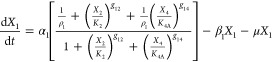
We start with a conceptual model for gene circuitry, such as those represented in Figure 1. This is converted to a mathematical model that typically involves ordinary differential equations with rational function nonlinearities for mRNA synthesis and linear functions for the other processes. The rational functions for regulation involving both activator and repressor represent the competition between formations of two mutually exclusive DNA loops.²⁴ For the particular case of a model such as that in Figure 1C

1

2

3

4

5

6

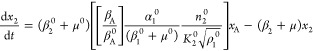
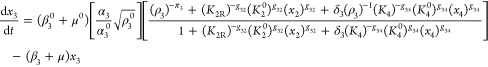
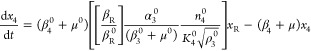
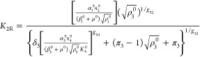
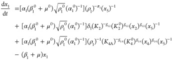
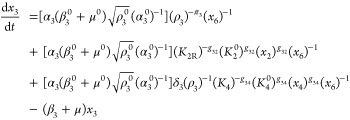
The interpretation of the symbols is as follows. X₁ and X₃ represent the concentration of activator and repressor mRNA, respectively; X₂ and X₄ represent the concentration of activator and repressor protein, respectively; X_A and X_R represent the concentration of immature forms of activator and repressor, respectively; α₁ and α₃ are maximum rates of transcription, the other α’s and the β’s are first-order rate constants, μ is the first-order rate constant for dilution due to exponential growth, ρ₁ = α₁/α₁^min and ρ₃ = α₃/α₃ are the regulatory capacities, the g’s are kinetic orders representing the cooperativity of repression or activation, and the K’s are concentrations of regulator for half-maximal binding to control sequences in the DNA (these concentrations for binding near their own promoter regions are given by K₂ and K₄ and for binding near the other promoter region are given by K_2R and K_4A).

Figure 1.

Three architectures and two modes for the molecular control of transcription manifested by two-gene circuits with an extra first-order process involved in the maturation of the functional form for each regulator. Architectures: (a) Negative feedback loop, (b) positive and negative feedback loops, and (c) positive and nested negative feedback loops. Combinations of two modes of molecular control: (d) activator-primary and (e) repressor-primary. The symbols are the following: NA, nucleic acid precursors; mRNA, messenger RNA; A, activator; R, repressor.

Nominal Parameter Values

For purposes of illustration, we shall use nominal parameter values based on information for the wild-type lac operon of Escherichia coli. The cooperativity for induction is 2;^25,26 the capacity for regulation is about 100;^25,26 the rate constant for mRNA decay is 20.8 h^–1;^27,28 the rate constant for loss due to dilution μ has a value of (ln 2)/T h^–1 in cells growing exponentially with a doubling time of T hours, and the ratio of protein to mRNA, n, is about 30.^29,30 The basal rate of the wild-type lac promoter yields approximately 10 molecules of β-galactosidase per cell.³¹ With ρ = 100, the maximum rate would yield approximately 10ρ/30 molecules of β-galactosidase mRNA per cell.

For a rational function with g = 2 and ρ = 100 and linear functions for the other processes, a 10-fold increase in the rate constant for loss of the repressor causes a 100-fold change from basal to maximal level of expression; a 10^1/2-fold increase yields expression that is the geometric mean between basal and maximal expression,¹⁹ which will become important in the normalization below. If we assume that the cells are growing with a doubling time T = 1 h and regulatory proteins are tagged to reduce their chemical half-life to 2/3 h,³² then we obtain the following nominal values for the parameters in eqs 7–12 and, with the exception of kinetic orders, denote them with the superscript (⁰): g_ij = 2 for the kinetic order parameters, ρ_2i–1⁰ = 100 for the regulatory capacities, μ⁰ = ln(2) = 0.693 for the rate of loss due to dilution, β_2i–1 = 20.8 h^–1 and β_2i⁰ = 1.5 ln(2)10^1/2 = 3.29 h^–1 for the rate constant parameters of mRNA and tagged proteins at midlevel expression, n_2i = 30 μ⁰/(β_2i⁰ + μ⁰) = 5.22 for the ratios of regulator to mRNA, and α_2i–1/(β_2i–1⁰ + μ⁰) = 33.3 mRNA molecules per cell. We also will examine various nominal values for the rate constants associated with maturation of the immature proteins, β_A and β_R⁰. Nominal values for several of the other parameters are unknown. However, their values can be used in a normalization process that eliminates these parameters from the resulting equations, which still retain the essential character of the original equations. This is a well-known general technique that simply scales the values of the system’s variables, and if the values of the parameters used in the normalization were to become known, then one could readily reconstruct the behavior of the original variables.

Parameters without the superscript are equal to the corresponding parameters with the superscript at a given nominal steady state. Parameters without the superscript are allowed to vary only in determining global tolerances of the systems at a given nominal steady state. It is important to realize that in the determination of global tolerances the corresponding superscripted parameters involved in the normalization are not allowed to change.

Normalized System Equations

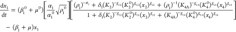
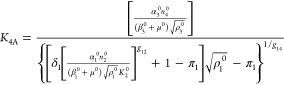
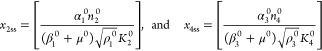
The variables in eqs 1–6 are normalized by making use of the steady state and the nominal parameter values in the previous subsection: The concentrations of the mRNAs are normalized with respect to the geometric mean of the expression extremes [α_2i–1⁰/(β_2i–1 + μ⁰) and [α_2i–1⁰/(β_2i–1 + μ⁰)]/ρ_2i–1⁰] at the nominal steady state, x_2i–1 = ((β_2i–1 + μ⁰)(ρ_2i–1⁰)^1/2/α_2i–1)X_2i–1. The concentrations of the immature forms of the activator and repressor are normalized with respect to their respective steady-state values, x_A = [(β₁⁰ + μ⁰)(β_A + μ⁰)(ρ₁⁰)^1/2/(α₁⁰α_A)]X_A and x_R = [(β₃⁰ + μ⁰)(β_R + μ⁰)(ρ₃⁰)^1/2/(α₃⁰α_R)]X_R. The concentrations of the regulators are normalized with respect to their effective DNA dissociation constant near the promoter region for their own transcription, x_2i = X_2i/K_2i⁰. We assume the same pair of binding sites for the repressor-DNA looping and the same pair of binding sites for activator-DNA looping at both promoters in the reference system (see Mathematically Controlled Comparisons), i.e., K_2R = K₂ and K_4A = K₄⁰ in the reference system. Moreover, given the values above for n_2i and ρ_2i–1⁰, the two binding constants for the reference system are related as follows

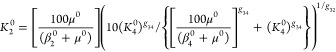or K₂⁰ ≈ 10^1/2K₄ when K₄⁰ ≪ 100 μ⁰/(β₄ + μ⁰). The value of K₄⁰ is a free parameter that maximizes the regions of oscillation when assigned a small value such as 0.5 molecules per cell.

This normalization places the steady-state value at the geometric mean of the regulatable region for each rational function (see Nominal Parameter Values), which maximizes the region of potential oscillation. Conversely, operation on the plateau of either function at either the basal or maximal level of expression greatly diminishes, and in most cases eliminates, the potential for sustained oscillation. As a necessary condition for limit-cycle oscillations the fixed point at the geometric mean should be an unstable focus. For systems that involve only two variables, an unstable focus provides a necessary condition for Hopf bifurcation and a stable limit cycle.³³ This can be extended to systems with additional variables by satisfying well-known conditions.^34,35

Although systems exhibiting sustained oscillation may have variables that operate only on the regulatable regions of the rational functions,³⁶ this need not be the case. Indeed, as we will see, dynamic excursions into the regions of saturation can limit the growing oscillations from an unstable focus and supply the sufficient conditions for a stable limit cycle.

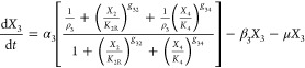
A normalized version of eqs 1–6, but generalized to account for the variations in design that are the focus of this article, is the following

7

8

9

10

11

12

where

13

and

14

The steady-state solution for eqs 7–12 is given by

The following binary parameters are used to denote the various designs that will be analyzed

In the Results and Discussion section, we refer to eqs 7–14 with various values for the parameters δ₁, δ₃, π₁, and π₃.

The result is still a system of nonlinear ordinary differential equations that is analytically intractable. Although there are various local methods for analytically examining particular fixed points and numerical approaches as well, each system is typically treated in an ad hoc fashion, and it remains a challenge to obtain a global perspective on the behavioral repertoire of such systems. However, we use a novel method of phenotypic deconstruction that greatly facilitates identification of the system’s qualitatively distinct phenotypes, which can then be examined in more detail with conventional methods.

Phenotypic Deconstruction

The first step in the phenotypic deconstruction of these nonlinear models is to recast them into a generic form known as a generalized mass action (GMA) system³⁷ in which the exponents need not be the small integer values of mass action systems but can be real numbers, including those with negative values. The system of ordinary differential eqs 7–12 can be recast exactly into an equivalent GMA system of differential-algebraic equations by simply defining the denominator of each rational function as a new variable,¹⁰ in this case x₅ and x₆.

15

16

17

18

19

20

21

22

This form provides the basis for a rigorous definition of phenotype and a method for deconstructing the original system into a collection of simpler nonlinear subsystems. In any given steady state, one term in each sum of a given sign has a larger value than the others in that sum. The dominant terms are retained, the nondominant terms are neglected, and the result is a unique subsystem (S-system) that defines a qualitatively distinct phenotype of the system.^9,10 The subsystem is a valid approximation of the full system if the conditions for term dominance are satisfied.

As an example, suppose the dominance involves the second term in eqs 15 and 18, the third term in eq 21, and the first term in eq 22. The resulting set of equations when the other terms are neglected is then the following

23

24

25

26

27

28

This nonlinear S-system combines the advantages of capturing essential nonlinear behavior locally while remaining analytically tractable. The explicit solution of eqs 23–28 gives the complete relationship between the steady-state values of the dependent state variables on the one hand and the values of the independent variables and parameters of the system on the other. The independent variables may be thought of as those that are determined by factors outside the system of interest, the environmentally determined variables. The parameters, which characterize the relatively fixed aspect of the system itself, may be thought of as genetically determined parameters.

There are a large number of combinations of potentially dominant terms and steady-state solutions for the corresponding S-systems. The total number of combinations is equal to the product of the number of terms of a given sign in each of the equations; in this case, the total is 5184. However, not all combinations of dominant terms are valid. To be valid, a particular combination must meet two requirements. First, the resulting S-system must have a steady-state solution. Second, given that solution, all of the other terms in a given sum must be smaller than the presumed dominant term. For example, if the second positive term in eq 15 is dominant, as was assumed above, then

29

Finding the valid combinations is a tractable linear programming problem^38,39 that involves solving the S-system equations (set of linear equations in log space) along with the dominance conditions (a set of linear inequalities in log space).^9,40 The resulting solutions provide a rigorous mathematical definition of the boundaries between regions of qualitatively distinct behavior for the system. These boundaries involve all of the environmentally determined variables and all of the genetically determined parameters of the system.

Once the boundaries have been determined for all the valid combinations of dominant terms, the results are integrated into a system design space. This space, with axes that represent the environmentally determined variables and the genetically determined parameters of the system, consists of space-filling irregular polytopes. Each point in this gene-by-environment space defines a distinct phenotype of the system that can vary quantitatively from one point to another. A qualitatively distinct phenotype is defined mathematically as the characteristic phenotype of the system that exists throughout a region of design space defined by the validity conditions, and the collection of qualitatively distinct phenotypes defines the full phenotypic repertoire of the system. For convenience in illustrating the relationships among genotype, environment, and phenotype, we typically choose to plot one of the genotypically determined parameters on the y axis, one of the environmentally determined variable on the x axis, and one of the phenotypic traits as a heat map on the z axis. Such a choice represents a particular “slice” through the fixed polytopes of the system design space. However, as noted in the introduction, for the class of oscillator designs considered here it is instructive to plot the rate constants for the functional inactivation of the regulators on the x and y axes. The growth rate dominates regulator loss (by dilution) whenever it is greater than the rate of functional loss (greater protein stability). For this reason, we plot values of β₂ and β₄ relative to the nominal growth rate μ⁰ and consider only positive ratios (see Results and Discussion, Figures 3–6).

Figure 3.

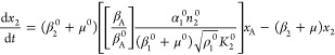
Gene circuit with a single negative feedback. (a) Circuit architecture with repressor-only control of activator transcription and activator-only control of repressor transcription. (b, c) System design space with the effective rate constant for inactivation of the activator, β₂, represented on the horizontal axis and that for the repressor, β₄, on the vertical axis. (b) Enumeration of the qualitatively distinct phenotypes identified by color, where the color bar represents the case number for each of the qualitatively distinct phenotypes. (c) The phenotypic trait represented as a heat map on the z axis of the system design space is the number of eigenvalues with positive real part. The color bar in this case represents the value of the phenotypic trait: blue for zero eigenvalues with positive real part (monostability), red for one eigenvalue with positive real part (bistability), and yellow for two complex eigenvalues with positive real part (unstable focus). (d) Temporal behavior of the full GMA system at the nominal operating point (●) within the region having the potential for sustained oscillation.

Figure 6.

Gene circuits with one positive and nested negative feedback loops: repressor-primary control of repressor transcription. (Left panel) Activator-primary control of activator transcription or (Right panel) repressor-primary control of activator transcription. See caption of Figure 3 for a description of panels a–d.

The system representation for each qualitatively distinct phenotype is always a simple S-system for which determination of its nonlinear behavior reduces to conventional linear analysis.^36,37 Thus, these phenotypes are completely determined, they can be analyzed in detail, and their relative fitness can be compared on the basis of relevant performance criteria. The properties and behaviors of a qualitatively distinct phenotype, e.g., local dynamics and steady-state behavior, are referred to as phenotypic traits. It must be emphasized that the boundaries are not arbitrary but are uniquely defined by the structure of the original equations. This provides an efficient and objective way of decomposing parameter space into a finite number of regions representing qualitatively distinct phenotypes, which greatly diminishes the sampling problem encountered with the conventional strategy described in the introduction. The boundaries determined in this manner tend to be conservative in that they provide regions in which necessary but not sufficient conditions exist for the realization of a specific phenotypic trait. Numerical simulations focused on these regions can then be used to determine whether the sufficient conditions are met. This combination of (1) deconstruction to focus the global exploration and (2) numerical simulation to refine experimental tests greatly facilitates the global characterization of the systems. To the best of our knowledge, there are no alternatives with these advantages.

Mathematically Controlled Comparisons

The comparisons in the Results and Discussion section utilize the method of mathematically controlled comparison, which consists of several steps that are described in detail elsewhere.^36,37,41 (1) The alternatives being compared are restricted to having differences in a single specific process that remains embedded within its natural milieu; this is the biological equivalent of a single mutation in an otherwise isogenic background. (2) The values of the parameters that characterize the unaltered processes of one system are assumed to be strictly identical with those of the corresponding parameters of the alternative system. This equivalence of parameter values within the systems is called internal equivalence. It provides a means of nullifying or diminishing the influence of the background, which in complex systems is largely unknown. (3) Parameters associated with the changed process are initially free to assume any value. This corresponds to the creation of extra degrees of freedom (think mutation). (4) The extra degrees of freedom are then systematically reduced (think selection) by imposing constraints on the external behavior of the systems; e.g., by insisting that the steady state be the same in the alternative systems. In this way, the two systems are made as nearly equivalent as possible in their interactions with the outside environment. This is called external equivalence. (5) The constraints imposed by external equivalence fix the values of the altered parameters in such a way that arbitrary differences in systemic behavior are eliminated. Functional differences that remain between alternative systems with maximum internal and external equivalence constitute irreducible differences. (6) When all degrees of freedom have been eliminated and the alternatives are as close to equivalent as they can be, then comparisons are made by mathematical and computer analyses of the alternatives.

The establishment of external equivalence is critically important in comparing nonlinear systems. It is used to establish the same nominal state for the systems being compared, i.e., to have the systems operating with the same values for their concentrations and fluxes. Failure to have the systems in the same nominal state can lead to an erroneous understanding of the results from the comparison. For example, in an amino acid biosynthetic pathway regulated both by repression at the genetic level and inhibition at the enzyme level (Figure 2a), a mutant with loss of feedback inhibition can exhibit oscillatory instability (Figure 2b). This might lead to the conclusion that the role of this feedback inhibition is ensuring stability of the system.⁴² However, for many feedback-resistant mutants, not all, the flux through the pathway can be much greater than that in the wild type; this leads to saturation of an enzyme downstream of the pathway (the aminoacyl-tRNA synthetase), and it is this saturation that can cause instability of an otherwise stable system. Once there is such an uncontrolled difference in the state of the nonlinear systems, such as the gross difference in pathway flux in this case, all bets are off. There can be secondary effects elsewhere in the system that can completely obscure the difference one is trying to understand.

Figure 2.

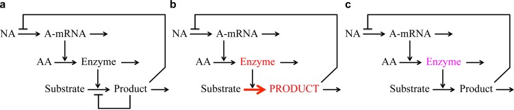
Importance of external equivalence for a mathematically controlled comparison. (a) Wild-type circuit for a stable amino acid biosynthetic system with repression at the gene level and end-product inhibition at the enzyme level. (b) A feedback-resistant mutant with loss of the binding site for the end product and an elevated (deinhibited) flux, an elevated concentration of product, saturation of the last enzyme (aminoacyl-tRNA synthetase), and oscillatory instability. (c) A feedback-resistant mutant with loss of the binding site for the end product and a concomitant reduction in molecular activity of the feedback-resistant enzyme. The resulting flux and concentration of product are identical to those of the wild type, and the system remains stable despite the loss of end-product inhibition.

A mathematically controlled comparison in this case would involve the equivalent of selecting a specific feedback-resistant mutant from the large class of such mutants. The parameters of this mutant enzyme would be altered to reflect not only loss of the recognition site for the end product of the pathway but also a reduced molecular activity such that pathway flux is the same as that in the wild-type organism (Figure 2c). That is, one of the constraints imposed by external equivalence to maintain the same nominal state of the systems being compared is that pathway flux be the same in the two systems. In such a well-controlled comparison, the downstream enzyme is not saturated, and there need be no oscillatory instability.

For a mathematically controlled comparison of alternative designs for a two-gene oscillator, we must consider changes in all of the parameters influencing the two transcription processes. The two critical constraints for external equivalence in this context are ensuring (a) that the alternative systems have the same nominal state and (b) that the nominal state is centered in the dynamic range of expression so as to maximize the potential for the oscillatory phenotype.

For convenience, and without loss of generality, the reference system selected for the normalizations and comparisons in this article has the following set of parameter values: δ₁ = δ₃ = π₁ = π₃ = 1. The constraints for external equivalence in making the mathematically controlled comparisons with the other cases are then the following

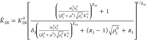30

31

where the parameters unique to the alternative designs are shown with a circumflex, and all other parameters are those of the reference system shown with the superscript ⁰.

There are changes among the unique parameters of the alternative designs, other than K̂_2R and K̂_4A, that one might consider; however, these are not able to satisfy the two critical constraints for external equivalence that are necessary for fair comparisons. For example, one might consider changes in α̂₁ and α̂₃, the maximal rates of regulator transcription, among the alternatives. However, these changes allow one to ensure only (a) that the alternative systems have the same nominal state but not (b) that the nominal state is centered in the dynamic range of expression.

Computational Procedures

System Design Space

We constructed and analyzed the system design space using the Design Space Toolbox for MATLAB 1.0⁴⁰ and extensions that are currently under development. All MATLAB computations were performed using MATLAB 7.8 (R2009a).

Routh Criteria for Local Stability

A linear system of differential equations in n variables has n Routh criteria of a given sign that can be calculated automatically.³⁶ The number of sign changes starting with the first criterion, which is positive, and progressing through the sequence from the first to the nth criterion indicates the number of eigenvalues with positive real part. If there are no sign changes, then the system is monostable. As parameters change and the system is becoming unstable, the first two criteria that change sign are the penultimate criterion and the last criterion;^43,44 for this reason, these are called the critical criteria. As the penultimate Routh criterion changes from positive through zero to negative, the system undergoes a Hopf bifurcation^45,46 to an unstable focus, a necessary condition for stable oscillation. As the last Routh criterion changes from positive through zero to negative, the system undergoes a saddle-point bifurcation^19,20,33 to an unstable node, a necessary condition for bistability. Applications of Routh criteria specifically in the context of gene circuitry can be found in refs (19−21, 36, and 40).

Numerical Methods

Computer simulations of the full nonlinear systems are performed with the SUNDIALS stiff solver, CVODE.⁴⁷ Global tolerances of the oscillatory phenotype are determined by numerical continuation in combination with a discrete fast Fourier transform using the numpy.fft algorithm in the NumPy library version 1.6.2.⁴⁸

Results and Discussion

We use the system design space methods to analyze gene circuits with three different architectures and various combinations of molecular modes for control of transcription. As with all of the systems analyzed to date, each of these variations in gene circuit design exhibits a unique phenotypic repertoire, much like a fingerprint.

Three Architectures

The three architectures that we shall analyze are shown schematically for a two-gene circuit in Figure 1. The architecture of a single negative feedback loop in which the first regulator is an activator and the second is a repressor is shown in Figure 1a. The architecture with a single negative feedback loop and a single positive feedback loop in which the first regulator also activates transcription of the first gene is shown in Figure 1b. The architecture with a single positive feedback loop in which the first regulator activates transcription of the first gene and a nesting of two negative feedback loops in which the second regulator represses transcription of both the first and the second gene is shown in Figure 1c.

Dual Modes of Molecular Control

It is important to note that there are dual modes for realizing molecular control of the same physiological function.

Regulation Involving Either Activator or Repressor

The lac operon and the mal operon of E. coli carry out the same physiological function, namely, inducible catabolism of their substrate. They both encode inducible disaccharidases, and yet the regulation of one is realized with a repressor and the other with an activator. It was once thought that these different modes of molecular control were the result of historical contingencies and that they conferred no functional differences upon the systems. It is now clear that the alternative modes exhibit functional differences that are accounted for by demand theory.⁴⁹⁻⁵² In brief, positive control tends to be selected when expression of the regulated genes is in high demand, and negative control, when expression of the regulated genes is in low demand.

Regulation Involving Combinations of Activator and Repressor

The abstract diagrams in Figures 1a–c, and most others found in the literature that are similar or simpler, do not distinguish between combinations of these dual modes for control. The depiction of regulatory interactions in these diagrams must therefore be refined to account for the different combinations. For example, there are alternative combinations for the control of the first gene in Figure 1b,c and the second gene in Figure 1c. In the first combination, which we call activator primary, the promoter is quiescent in the absence of both regulators. The activator is the primary regulator necessary to increase expression from the promoter; the repressor in this case is the secondary regulator that “antagonizes” the activity of the activator to bring about repression of an otherwise activated promoter (Figure 1d). In the second combination, which we call repressor primary, the promoter is fully active in the absence of both regulators. The repressor is the primary regulator necessary to reduce expression from the promoter; the activator in this case is the secondary regulator that “antagonizes” the activity of the repressor to bring about activation of an otherwise repressed promoter (Figure 1e).

Could these generic differences in molecular interaction have an impact on the phenotype of otherwise equivalent gene circuits? And might the choice be at least partially responsible for differing degrees of experimental success in realizing synthetic constructs? We will address these questions in the analyses that follow. In each case, we follow the strategy as outlined in the Introduction. First, a mathematical model is formulated and represented graphically, panel a of Figures 3–6, that summarize our results. Second, the qualitatively distinct phenotypes are identified and enumerated by construction of the system design space, which represents each of these phenotypes by a colored region, panel b of Figures 3–6. Third, a particular trait of each phenotype (here the number of eigenvalues with positive real part for the corresponding subsystem in each region, with two providing a necessary condition for limit-cycle oscillation) is plotted as a heat map on the z axis of the system design space, panel c of Figures 3–6. Finally, the dynamics of the full model are examined numerically in regions of interest to determine if the necessary conditions for oscillation are also sufficient and a representative example of the dynamics is plotted, panel d of Figures 3–6.

It is important to note that the necessary conditions established in step 3 are obtained from the Routh criteria (bifurcation analysis) for the subsystem in the region with potential for limit-cycle behavior and not from the full model. It is only with a focused analysis of the full model in step 4 that the sufficient conditions are established. A detailed comparison of bifurcation analysis involving a full model and its relevant subsystems is provided elsewhere.¹⁰

Single Negative Feedback Loop (S.1)

A conventional model for the circuit with this architecture (Figure 3a) involves rational function nonlinearities for mRNA synthesis and linear functions for the other processes, and it is described in the Methods section (eqs 15–22, 30, and 31, with δ₁ = 0, δ₃ = 0, π₁ = 0, and π₃ = 1). The system design space for this circuit exhibits 5 qualitatively distinct phenotypes with valid regions radiating from the region at the origin (Figure 3b). Each phenotypic region corresponds to a unique subsystem with unique traits, such as signal amplification factors. For example, the amplification factor between an input signal (represented by changes in activator lifetime) and an output signal (represented by the repressor concentration) has a different functional form in different phenotypic regions. The amplification factor in the region indicated by case number 3 (subsystem given by the first positive term in eqs 15, 21, and 22 and by the second positive term in eq 18) is an inverse quadratic function, whereas that the region indicated by case number 4 (subsystem given by the first positive term in eqs 15 and 21 and the second positive term in eqs 18 and 22) is a zero-order function.

The qualitatively distinct phenotypes can be compared on the basis of other traits, such as the dynamic behavior about their fixed points. All of the peripheral regions correspond to phenotypes that have a monostable trait, whereas the region at the origin has the possibility of representing a sustained oscillatory trait, provided the critical conditions for an unstable focus are met (e.g., all Routh criteria satisfied except the penultimate one [see Methods section]). Indeed, the Routh criteria provide necessary conditions for identifying simple and higher-order Hopf bifurcations in n-dimensional systems.^45,46 Given the nominal parameter values in the Methods section with delays for both activator and repressor maturation approximately equal to the protein lifetimes, the necessary Routh conditions are met for a small region (Figure 3c). However, it must be stressed that detailed analysis of the full system in this region shows that the potential is overestimated and the sufficient conditions for limit-cycle oscillation are not satisfied. Therefore, the circuit fails to exhibit sustained oscillations (e.g., Figure 3d).

Single Positive and Negative Feedback Loops: Activator-Only Control of Repressor Transcription

Relaxation oscillators have more complex feedback circuitry involving coupled positive and negative feedback interactions. Such coupled feedback circuitry is abundant in nature from bacteria to humans. The principle examples, which have been treated extensively, are circadian circuits^53,54 and cell cycle circuits.^55,56 There also has been a long prior history of their analysis in electronic circuits such as the famous Van der Pol oscillator.⁵⁷ Again, the critical last two Routh conditions⁴⁴ play an important role in characterizing the fixed points of such systems. Unlike the circuit in the previous section, in which a single regulator is involved in the control of each transcriptional unit, there are alternative realizations of the circuits in this section.

Activator-Primary Control of Activator Transcription (S.2)

The model involving rational function nonlinearities for the activator-primary control of activator transcription (Figure 4a, left) is presented in the Methods section (eqs 15–22, 30, and 31, with δ₁ = 1, δ₃ = 0, π₁ = 1 and π₃ = 1). The system design space of the activator-primary circuit consists of a number of qualitatively distinct phenotypes that are valid within nonoverlapping as well as overlapping regions (Figure 4b, left). This circuit has the potential for realizing phenotypes with all three of the dynamic traits suggested by theory.²⁴ Other than the phenotypic regions with a monostable trait, this circuit is dominated by a phenotypic region with the potential for sustained oscillation, sandwiched between regions with a bistable trait. Given the nominal parameter values in the Methods section with delays for both activator and repressor maturation approximately equal to the protein lifetimes, the critical Routh conditions are met essentially for the entire region with potential for oscillation (Figure 4c, left). Detailed analysis of the full system in this region shows that this circuit does indeed exhibit sustained oscillations over a large portion of the region (e.g., Figure 4d, left).

Figure 4.

Gene circuits with one positive and one negative feedback loop. Activator-only control of repressor transcription and (Left panel) activator-primary control of activator transcription or (Right panel) repressor-primary control of activator transcription. See caption of Figure 3 for a description of panels a–d.

Repressor-Primary Control of Activator Transcription (S.3)

The model involving rational function nonlinearities for the repressor-primary control of activator transcription (Figure 4a, right) is presented in the Methods section (eqs 15–22, 30, and 31, with δ₁ = 1, δ₃ = 0, π₁ = 0, and π₃ = 1). The system design space of the repressor-primary circuit consists of a number of nonoverlapping as well as overlapping phenotypic regions, and this circuit is also capable of realizing all three of the dynamic traits. Again, other than the qualitative phenotypes that have a monostable trait, this circuit is dominated by a phenotypic region with the potential for sustained oscillation, sandwiched between regions of bistability (Figure 4b, right). Given the nominal parameter values in the Methods section with delays for both activator and repressor maturation approximately equal to the protein lifetimes, the critical Routh conditions for sustained oscillations are met essentially for the entire region of potential oscillation (Figure 4c, right). Detailed analysis of the full system in this region shows that this circuit also exhibits sustained oscillations throughout (e.g., Figure 4d, right).

Note that the region of potential sustained oscillations for the repressor-primary circuit (Figure 4c, right) is larger than that for the activator-primary circuit (Figure 4c, left). Moreover, unlike the circuitry in Figure 3A, the circuitry in this section can achieve sustained oscillations essentially throughout the region of potential limit-cycle oscillation. This is a measure of the increase robustness of relaxation oscillators (see also Global Tolerances, Figure 7).

Figure 7.

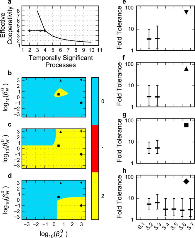
Influence of delay on oscillatory potential and circuit robustness. (a) Trade-off between number of temporally significant processes (delay) and effective cooperativity of the feedback^59,64 in a negative feedback circuit analogous to that in Figure 3A. The arrow represents changes discussed in the text. (b–d) Comparison of regions representing potential for sustained oscillation as a function of delay associated with the rate constants for maturation of activator, β_A⁰ on the x axis, and repressor, β_R on the y axis: (▼) both maturation delays negligible, (▲) repressor maturation delay negligible and activator maturation delay approximately equal to protein turnover time, (■) both maturation delays equal to protein turnover time, and (◆) activator maturation delay negligible and repressor maturation delay greater than protein turnover time. The color bar represents the value of the phenotypic trait: blue for zero eigenvalues with positive real part (monostability), red for one eigenvalue with positive real part (bistability), and yellow for two complex eigenvalues with positive real part (unstable focus). (b) Circuit with a single negative feedback, (c) circuits with one positive and one negative feedback, and (d) circuits with one positive and nested negative feedbacks. (e–h) Global tolerances for the oscillatory phenotype of the full GMA systems with various designs: (S.1) activator-only control of repressor transcription and repressor-only control of activator transcription; activator-only control of repressor transcription and (S.2) activator-primary control of activator transcription or (S.3) repressor-primary control of activator transcription; activator-primary control of repressor transcription and (S.4) activator-primary control of activator transcription or (S.5) repressor-primary control of activator transcription; repressor-primary control of repressor transcription and (S.6) activator-primary control of activator transcription or (S.7) repressor-primary control of activator transcription. Mean, maximum, and minimum fold tolerances (excluding infinite values) are given for the increase and decrease in the 14 parameters of systems S.2 and S.3 and in the 15 parameters of systems S.4–S.7: (e) both maturation delays negligible; (f) repressor maturation delay negligible and activator maturation delay equal to protein turnover time; (g) both maturation delays equal to protein turnover time; (h) activator maturation delay negligible and repressor maturation delay greater than protein turnover time.

Positive and Nested Negative Feedback Loops: Activator-Primary Control of Repressor Transcription

There are two fundamentally different classes of circuitry when the transcription of both activator and repressor involves both activator and repressor control, depending on the primary mode of control for repressor transcription. In one, the repressor is controlled by an activator-primary mechanism, the class considered in this section. In the other, which is treated in the following section, it is controlled by a repressor-primary mechanism.

Activator-Primary Control of Activator Transcription (S.4)

The architecture in this case involves rational function nonlinearities for the activator-primary control of both transcripts (Figure 5a, left). The equations for this circuit, which provide the arbitrary reference in our comparisons, are presented in the Methods section (eqs 15–22, 30, and 31, with δ₁ = 1, δ₃ = 1, π₁ = 1, and π₃ = 1). The system design space for this circuit exhibits several nonoverlapping monostable phenotypic regions surrounding a band of three regions composed of one potential oscillatory region and two bistable regions (Figure 5b, left). The sustained oscillatory phenotype would require that the critical conditions be met (i.e., all Routh criteria satisfied except the penultimate one). Given the nominal parameter values in the Methods section with additional delay for repressor maturation but not activator maturation, the critical Routh conditions are met for a slice of the region (Figure 5c, left). Detailed analysis of the full system in this region shows that this circuit exhibits sustained oscillation, as shown in Figure 5d, left.

Figure 5.

Gene circuits with one positive and nested negative feedback loops: activator-primary control of repressor transcription. (Left panel) Activator-primary control of activator transcription or (Right panel) repressor-primary control of activator transcription. See caption of Figure 3 for a description of panels a–d.

Repressor-Primary Control of Activator Transcription (S.5)

The architecture in this case involves rational function nonlinearities for the activator-primary control of the repressor transcript and repressor-primary control of the activator transcript (Figure 5a, right). The equations for this circuit are presented in the Methods section (eqs 15–22, 30, and 31, with δ₁ = 1, δ₃ = 1, π₁ = 0, and π₃ = 1). The system design space for this circuit exhibits several nonoverlapping monostable phenotypic regions surrounding a potential oscillatory region (Figure 5b, right). The sustained oscillatory phenotype would require that the critical conditions be met. Given the nominal parameter values in the Methods section with delay for repressor maturation but not activator maturation, the critical Routh conditions are met for a slice of the region (Figure 5c, right). Detailed analysis of the full systems in this region shows that this circuit also exhibits sustained oscillation, as shown in Figure 5d, right.

Positive and Nested Negative Feedback Loops: Repressor-Primary Control of Repressor Transcription

As noted in the previous section, there are two fundamentally different classes of circuitry when the transcription of both activator and repressor involves both activator and repressor, depending on the primary mode of control for repressor transcription. In this section, we examine the class in which repressor transcription is controlled by a repressor-primary mechanism. Activator transcription can be controlled by either an activator- or repressor-primary mechanism.

Activator-Primary Control of Activator Transcription (S.6)

The model involving rational function nonlinearities for the activator-primary control of the activator transcript and repressor-primary control of the repressor transcript is shown in Figure 6a, left. The equations for this circuit are presented in the Methods section (eqs 15–22, 30, and 31, with δ₁ = 1, δ₃ = 1, π₁ = 1, and π₃ = 0). The system design space for this circuit exhibits several nonoverlapping monostable phenotypic regions surrounding a band consisting of a region representing a potential oscillatory phenotype and two representing bistable regions (Figure 6b, left). The sustained oscillatory phenotype would require that the critical conditions be met (i.e., all Routh criteria satisfied except the penultimate one). Given the parameter values in the Methods section with delay for repressor maturation but not activator maturation, the critical Routh conditions are met for a slice of the region (Figure 6c, left). Detailed analysis of the full system in this region shows that this circuit is capable of exhibiting sustained oscillations, as shown in Figure 6d, left.

Repressor-Primary Control of Activator Transcription (S.7)

The architecture in this case involves rational function nonlinearities for the repressor-primary control of both transcripts (Figure 6a, right). The equations for this circuit are presented in the Methods section (eqs 15–22, 30, and 31, with δ₁ = 1, δ₃ = 1, π₁ = 0, and π₃ = 0). The system design space of the circuit with repressor-primary control of activator transcription consists of several nonoverlapping monostable regions surrounding a region with oscillatory potential (Figure 6b, right). The sustained oscillatory trait would require that the critical conditions be met. Given the parameter values in the Methods section with delay for repressor maturation but not activator maturation, the critical Routh conditions are met for a slice of the region (Figure 6c, right). Detailed analysis of the full system in this region shows that this circuit also is capable of exhibiting sustained oscillations, as shown in Figure 6d, right.

Comparisons

The method of mathematically controlled comparison ensures that the circuits analyzed in the previous sections are in the same nominal steady state at the geometric mean of their operating range to allow the maximum potential for cooperativity to manifest a stable limit cycle (see Methods). All of the circuits have the same steady-state concentrations of and fluxes through the mRNA and regulator pools. The concentrations of the immature proteins will necessarily differ with the magnitude of the delays; however, the systems being compared with the same delay all have the same nominal steady state. The comparisons also are controlled for number of kinetic steps and values of the parameters. Nevertheless, there are generic differences that remain regarding requirements for specific delays and the magnitudes of global robustness for the oscillatory phenotype, and the results of careful comparison suggest a best design among the alternatives.

Delay

A Hopf bifurcation to oscillation^33,58 is indicated, in the case of an nth-order negative feedback system analogous to that in Figure 3a, when all n Routh criteria are positive, excepting a negative penultimate criterion. The factors that influence these mathematical conditions are the effective strength of the net negative cooperativity, the number of processes in the feedback loop, and differences in values for the kinetic parameters of these processes. The conditions favoring oscillations are strong cooperativity, many intervening processes, and similar values for the kinetic parameters of the processes.⁵⁹ There is a trade-off in the critical condition for oscillatory instability between the number of temporally significant processes (the effective number of processes with the smallest comparable eigenvalues), which is related to the extent of delay in the feedback loop, and the effective cooperativity, which is related to the amplification in the feedback loop (Figure 7a).

Although the net cooperativity is 4 for the circuit in Figure 3A, the lifetimes of the mRNAs are 30 times shorter than those of the proteins, which reduces the number of temporally significant processes in the feedback loop to ∼2. Thus, from the trade-off curve in Figure 7a, the threshold for sustained oscillations could be reached by effectively adding two temporally significant processes in the loop. This might be achieved in several ways, by increasing the growth rate (which decreases the turnover time of the stable regulators) or tagging proteins for active degradation,³² which would tend to make four lifetimes more similar on the scale of mRNA turnover time. Alternatively, physically adding two linear processes with time constants (1/rate constants) comparable to protein turnover time would tend to make four lifetimes more similar on the scale of protein turnover time without changing the net cooperativity. In all of these cases, the time-scale separation would be reduced, and the number of temporally significant processes in the feedback loop, increased. In fact, all of our circuits include the possibility of an additional first-order process in the synthesis of both activator and repressor.

Even though the comparisons have been controlled for number of kinetic steps, parameter values, and cooperativity, it is not possible for all of the circuits to be compared with the same values for the additional delays and still exhibit sustained oscillations. Therefore, if we are to allow the alternatives to manifest their maximum potential for sustained oscillation, then we must allow them to differ with regard to the delays associated with the maturation of activator and repressor.

The only way that the circuit in Figure 3A might exhibit sustained oscillations is when the number of temporally significant processes for this circuit is increased to four and the circuit crosses the threshold for oscillatory instability (arrow in Figure 7a). This occurs when the two additional time constants are similar to those for protein turnover (■ in Figure 7b). Only then does this circuit exhibit the potential for sustained oscillations. However, detailed analysis of the full system (S.1) shows that this potential is overestimated and there is only damped oscillation (Figure 3D).

The circuits with positive and only one negative feedback (S.2 and S.3) exhibit robust sustained oscillations over a much wider range of delays (Figure 7c). Indeed, sustained oscillations are produced even when the delays associated with the additional first-order processes are eliminated (▼ in Figure 7c). The only way to eliminate sustained oscillations in these circuits is to have the rate constant for repressor maturation very large and that for the activator maturation very small (upper left portion of Figure 7c).

The circuits with positive and nested negative feedback (S.4 through S.7) cannot exhibit sustained oscillations when the additional delays associated with the maturation processes are eliminated (▼ in Figure 7d). There are two reasons for this. First, removing all feedback except for repression of activator transcription would leave only two temporally significant processes, which can never exhibit sustained oscillations.^36,60 Second, adding autorepression of repressor transcription produces an “inner” negative feedback that mathematically controlled comparisons have shown to be a stabilizing influence,^36,60 making it even more difficult to produce sustained oscillations.

In fact, for these circuits in which all message lifetimes (β₁ = β₃ = β_odd), protein lifetimes (β₂ = β₄ = β_even), and regulatory interactions (g₁₂ = g₃₂ = g₁₄ = g₃₄ = g) are identical, the circuits are always stable because all the Routh criteria^43,44 are satisfied for all combinations of values for these three classes of parameters. Thus, there is no possibility of these circuits exhibiting a sustained oscillatory phenotype, regardless of changes in growth rate or changes in regulator cooperativity or lifetime. The only way that these circuits can exhibit sustained oscillations is to ensure that the additional delay for the repressor maturation process is sufficiently long and greater than that for the activator maturation process (◆ in Figure 7d).

Global Tolerances of the Oscillatory Phenotype

The global tolerance to a change in phenotype caused by the change in value of a system parameter or environmental variable is defined as the maximum ratio of the value measured at the operating point and at the boundary to an adjacent phenotypic region.⁶¹ The global tolerances with respect to regulator half-life (which is readily tunable for regulators that have gratuitous activating or inactivating ligands) are evident from the particular slice of the system design spaces in Figures 3c–6c. The global tolerances with respect to the other parameters can be readily examined in a similar fashion by examining other slices. Tolerances for the maturation rate constants of repressor, β_R⁰, and activator, β_A, can be infinite. Thus, we exclude these parameters from the graphical summary of the global tolerances given in Figures 7e–h for selected values of the two delays. The results, which are then biased downward, apply only to the remaining 14 parameters of systems S.1 and S.2 and the 15 parameters of systems S.4–S.7.

When both additional delays have negligible values (▼ in Figure 7b–d), the only circuits capable of producing sustained oscillations are those with activator-only control of repressor transcription and either activator-primary (S.2) or repressor-primary (S.3) control of activator transcription. In Figure 7e, the mean values for their tolerances are 3.5- and 3.7-fold, respectively, and their most critical parameter has a relatively low value of 1.3- and 1.3-fold, respectively. The tolerances of the oscillatory phenotype for all the other circuits (S.1 and S.4–S.7) are zero, since they are incapable of oscillating without additional delay. The critical and mean global tolerances for the alternative designs at the delays shown in Figure 7 are compared in Table 1.

Table 1. Global Tolerance of the Oscillatory Phenotype for Each System as a Function of Delays Associated with Maturation of Activator and Repressor^a.

	maturation delay
system	▼	▲	■	◆
S.1	–	–	–	–
S.2	3.5/1.3	3.0/1.2	5.0/2.9	5.4/3.2
S.3	3.7/1.3	3.0/1.2	5.3/2.9	6.4/3.2
S.4	–	–	–	3.1/1.5
S.5	–	–	–	3.2/1.5
S.6	–	–	–	2.8/1.4
S.7	–	–	–	3.0/1.4

^aThe table shows the mean/minimum global tolerance for all the parameters of each system with the delays that correspond to those in Figure 7. The dash indicates the absence of an oscillatory phenotype.

To summarize, the circuit with repressor-primary control of activator transcription and activator-only control of repressor transcription is the most robust design based on the results above. It is one of the two options among the alternatives that exhibits sustained oscillations under almost any combination of delays, or no additional delays at all, involving maturation of activator and repressor. Furthermore, under delays that allow sustained oscillations in one or more of the alternatives, its average tolerance of the oscillatory phenotype is typically greater as is the tolerance of the most critical parameter. It also should be noted that in all cases the tolerances with respect to the rates of regulator degradation are actually underestimated compared to what would be expected if the concentration of the gratuitous environmental ligand were plotted on the axes. This is because we have assumed that the rate of regulator degradation is proportional to these concentrations, when in fact it will require larger increases in these concentrations as diminishing returns set in on the approach to saturation. The lower bound on these tolerances is set by the growth rate.

Circuits with and without the Nested Negative Feedback Loop

The mathematically controlled comparison of the alternative circuitry having activator-primary control of activator transcription with and without the nested negative feedback uses the constraint in eq 30 to fix the value K̂_2R in the circuit with activator-only regulation of repressor transcription (see Methods section). When this constraint is imposed, the two circuits have the same concentrations and fluxes at the nominal steady state. A comparison of the results for the alternative circuits having activator-primary control of activator transcription, with and without the nested negative feedback (left panels in Figures 5 and 4), shows that the presence of the nested negative feedback is a stabilizing influence that diminishes the size of the region with potential for sustained oscillation. Indeed, for the circuits with nested negative feedback, there are no stable oscillations unless the appropriate delays are included (see Figure 7d). When considering the maximum potential for sustained oscillation with the critical delays included, the tolerances for the circuit with the nested negative feedback (Figure 7h (S.4): mean = 3.1 fold) are smaller than those for the circuit without this feedback (Figure 7h (S.2): mean = 5.4 fold), which indicates a loss of global robustness. The results obtained for the alternative circuits having repressor-primary control of activator transcription, with and without the nested negative feedback, are shown in the right panels of Figures 4 and 5. The presence of the nested negative feedback is a stabilizing influence that diminishes the size of the region with potential for sustained oscillation. Again, there are no stable oscillations for the circuits with nested negative feedback unless the appropriate delays are included (see Figure 7d). When these delays are included, the tolerances for the circuit with the nested negative feedback (Figure 7h (S.5): mean = 3.2 fold) are smaller than those for the circuit without this feedback (Figure 7h (S.3): mean = 6.4 fold), which again indicates a loss of global robustness.

A mathematically controlled comparison of alternative circuitry having repressor-primary control of repressor transcription with and without the nested negative feedback cannot be made because there is no circuit corresponding to Figure 6a, right, if the nested negative feedback is eliminated. Removal of the “inner” negative feedback would leave the activator with no influence over the constitutive expression of repressor transcription.

Insights in the Context of Synthetic Projects Aimed at Realizing Robust Oscillations

The results for the negative feedback circuit show that too much or too little delay and there is no potential for sustained oscillations. The potential for sustained oscillations occurs only when the maturation delays for both the repressor and activator are similar to the turnover times of these proteins. Even then, this circuit is incapable of sustained oscillation. These results show that the pioneering synthetic construct of Elowitz and Leibler⁶² in E. coli might not have achieved sustained oscillations with the two-gene circuit in our analysis. However, they did achieve sustained oscillations with a three-gene (net-negative) circuit that also involved regulators tagged to shorten their lifetimes. In this circuit, the effective cooperativity would be 6, and the number of temporally significant steps would be ∼6 on the time scale of protein turnover; thus, the operating point of this circuit would be placed well above the threshold for oscillatory instability in Figure 7a.

Analysis in system design space demonstrates that robust sustained oscillations are realized more easily in circuits with positive as well as negative feedback compared with negative-only feedback circuits, provided the comparisons are well-controlled. Moreover, among the dual means of realizing the primary control of activator transcription, repressor-primary control (mean global tolerances 6.4-fold) is better than activator-primary control (mean global tolerances 5.4-fold) because of the larger range of feasible values for the parameters. These results for the activator-primary circuit (Figure 4a, left) suggest that the synthetic construct of Atkinson et al.²⁴ in E. coli, which produced robust oscillations that damped out after several cycles, might have yielded sustained oscillations if it had been appropriately tuned. However, the results also suggest that a more promising construct would utilize repressor-primary (Figure 4a, right) rather than activator-primary (Figure 4a, left) control of activator transcription.

The results for circuits with nested negative feedback loops demonstrate that sustained oscillations are more difficult to achieve when there is also a second negative feedback loop involving repressor transcription. The combination of activator-primary control of activator transcription and repressor-primary control of repressor transcription (S.6) is the worst of the six possibilities that produce oscillations (mean global tolerances 2.8-fold), whereas the combination of repressor-primary control of activator transcription and activator-only control of repressor transcription is the best of the six possibilities (mean global tolerances 6.4-fold). Thus, it is best not to include the second negative feedback and to have repressor-primary control of activator transcription.

As explained above, autorepression of repressor transcription reduces the potential for sustained oscillations. However, if additional temporally significant processes are incorporated into the positive and negative feedback loops of the models, as in Figures 5 and 6, then the augmented circuits are capable of generating sustained oscillations provided the delay is longer in the negative feedback loop (Figure 7d). With no delay (large rate constants for the additional processes in both the negative (β_R⁰) and positive (β_A) feedback loops) or equal delay in both loops, there are no sustained oscillations. Only with a large rate constant for the process in the positive loop and a small rate constant in the negative loop does the system exhibit sustained oscillations. In other words, if the delay in the positive feedback loop is sufficiently long, then it tends to diminish the effect of additional delay in the negative feedback loop. As long as there is more delay in the negative loop than in the positive loop, then oscillator behavior is facilitated.

A circuit with architecture similar to that in Figure 5a, left, with activator-primary control of both activator and repressor transcription, was constructed and studied in mammalian cells by Tigges et al.⁶³ Their construct differs by the inclusion of an extra transcriptional unit in the negative feedback loop and antisense RNA, rather then a repressor, to realize the nested negative interactions. The requirement for longer delay in the negative versus positive loop to facilitate oscillations would naturally be favored by the additional processes in the negative feedback loop of their construct. Although this model is not included within the framework of our well-controlled comparisons, preliminary analysis suggests similar results.

Stricker et al.²² developed a construct in E. coli with a hybrid promoter exhibiting a high basal rate of transcription. The basal rate of transcription can be downregulated and is consistent with a repressor-primary mode of control of both the activator and repressor (Figure 6a, right). However, the hybrid promoter can also be upregulated from the basal rate and may inherit some of the properties of the circuit with activator-primary control of both activator and repressor (Figure 5a, left). The observed oscillations were accounted for by including in their model processes such as protein folding, multimerization, and DNA looping. As long as there is more delay in the negative feedback loop than in the positive loop, then oscillatory behavior is favored for either circuit (Figure 7d). This was the case in the model of Stricker et al.,²² as they explained, because dimerization of AraC is faster than dimerization plus tetramerization of LacI.

Conclusions

The strategy used for the analysis in this article differs from the conventional strategy outlined in the introduction and offers a number of advantages. Although the fist step of model formulation is the same, the strategies differ fundamentally thereafter. In the second step, rather than performing a detailed analysis of the full model at sparsely sampled point of parameter space, our strategy automatically deconstructs the entire parameter space into a finite number of regions with rigorously defined boundaries (space-filling polytopes) that represent qualitatively distinct phenotypes associated with nonlinear subsystems. This greatly diminishes the sampling problem associated with the conventional strategy. In the third step, the conventional strategy involves decisions concerning which regions in parameter space to refine by a detailed analysis to identify boundaries between regions of interest (e.g, typical bifurcation analysis). In our strategy, this decision has already been made, and a simpler analysis (often involving a single analytical treatment that applies to an entire region) is used to characterize large chunks of parameter space in an approximate fashion to identify regions of interest. In the final step, the conventional strategy classifies different dynamical behaviors associated with particular regions of parameter space, whereas at this step, our strategy finally applies conventional methods to examine the behavior of the full model in detail, but it is focused only on regions already identified as being of interest.

In this article, we utilized a method of system deconstruction based on differences in phenotype, rather than the traditional approaches to deconstruction based on space, time, or function. This also can be viewed as a novel method for model reduction. The integration of phenotypes into a system design space allows the qualitatively distinct phenotypes to be identified, enumerated, characterized, and compared. The system design space provides an efficient means to characterize system behavior over a broad range of parameter values, and the landmarks in this space represent particular constellations of parameters that define relevant design principles. These characteristics facilitate the rapid generation of alternative hypothesis for experimental testing; in particular, they identify designs that are more promising because the range of realizable values for the parameters is larger than that of the alternatives.

This methodology provides an efficient strategy for obtaining a global perspective on the entire behavioral repertoire of a system and differs fundamentally from traditional approaches that first and foremost involve parameter estimation and sampling with no clear picture of the overall landscape. Our strategy rapidly identifies regions of system design space associated with each of the qualitatively distinct phenotypes; those regions of particular interest can be further characterized by an analytical treatment of the corresponding subsystems, and the full system can be examined in greater detail to test quantitative predictions as needed. This strategy provides key information regarding the range of potential behaviors that a model can exhibit, both desirable to be achieved as well as undesirable to be avoided. This allows for a directed approach to obtaining parameter values and limits the computational effort needed for a detailed analysis of system behavior.

Here, the method identified regions of potential limit-cycle oscillation. Further characterization revealed the local region in which necessary conditions for limit-cycle oscillation were met. Detailed analysis of the full systems in the local region provided sufficient conditions for sustained oscillations. Moreover, the detailed analysis showed that although the size of the local region was overestimated, oscillatory behavior, if it exists, can be found somewhere within the identified region. This has been true in other applications as well.^10,22 In this sense, the method tends to be conservative, overestimating the potential such that relevant behaviors are not overlooked. Although we made use of known parameter values in this application, knowledge of specific parameter values is not necessary. Our strategy is able to automatically identify a set of parameter values for each of the seven circuit designs that will locate their nominal operating point within a region of system design space having the potential for sustained oscillatory behavior.

There are, of course, obvious differences in the cellular context of all of the synthetic constructs. Aside from ad hoc differences due to the complex intracellular milieu and the details of the molecular elements in the constructs, our results reveal generic differences in the designs that might also have contributed to the differences in outcome. Comparison of the results for the seven different designs suggests that constructs employing repressor-primary control of activator transcription and activator-only control of repressor transcription could more readily realize a robust oscillator. Finally, it should be emphasized that the methods employed in this article are quite general and could be used for the analysis and comparison of other types of system as well as other gene circuit designs.

The authors declare no competing financial interest.

Funding Statement

National Institutes of Health, United States

References

- Novák B.; Tyson J. J. (2008) Design principles of biochemical oscillators. Nat. Rev. Mol. Cell Biol. 9, 981–991. [DOI] [PMC free article] [PubMed] [Google Scholar]
- Tsai T. Y.-C.; Choi Y. S.; Ma W.; Pomerening J. R.; Tang C.; Ferrell J. E. Jr. (2008) Robust, tunable biological oscillations from interlinked positive and negative feedback loops. Science 321, 126–129. [DOI] [PMC free article] [PubMed] [Google Scholar]
- Mukherji S.; van Oudenaarden A. (2009) Synthetic biology: understanding biological design from synthetic circuits. Nat. Rev. Genet. 10, 859–871. [DOI] [PMC free article] [PubMed] [Google Scholar]
- Purcell O.; Savery N. J.; Grierson C. S.; di Bernardo M. (2010) A comparative analysis of synthetic genetic oscillators. J. R. Soc., Interface 7, 1503–1524. [DOI] [PMC free article] [PubMed] [Google Scholar]
- Lenz P.; Søgaard-Andersen L. (2011) Temporal and spatial oscillations in bacteria. Nat. Rev. Microbiol. 9, 565–577. [DOI] [PubMed] [Google Scholar]
- Tigges M.; Dénervaud N.; Greber D.; Stelling J.; Fussenegger M. (2010) A synthetic low-frequency mammalian oscillator. Nucleic Acids Res. 38, 2702–2711. [DOI] [PMC free article] [PubMed] [Google Scholar]
- Kim J. K.; Forger D. B. (2012) A mechanism for robust circadian timekeeping via stoichiometric balance. Mol. Syst. Biol. 8, 630. [DOI] [PMC free article] [PubMed] [Google Scholar]
- Benner S. A.; Sismour A. M. (2005) Synthetic biology. Nat. Rev. Genet. 6, 533–543. [DOI] [PMC free article] [PubMed] [Google Scholar]
- Savageau M. A.; Coelho P. M. B. M.; Fasani R. A.; Tolla D. A.; Salvador A. (2009) Phenotypes and tolerances in the design space of biochemical systems. Proc. Natl. Acad. Sci. U.S.A. 106, 6435–6440. [DOI] [PMC free article] [PubMed] [Google Scholar]
- Lomnitz J. G.; Savageau M. A. (2013) Phenotypic deconstruction of gene circuitry. Chaos 23, 025108. [DOI] [PMC free article] [PubMed] [Google Scholar]
- Srere P. A.; Mosbach K. (1974) Metabolic compartmentation: symbiotic, organellar, multienzymic, and microenvironmental. Annu. Rev. Microbiol. 28, 61–83. [DOI] [PubMed] [Google Scholar]
- Waddington C. H. (1957) The Strategy of the Genes: A Discussion of Some Aspects of Theoretical Biology, Allen & Unwin, London. [Google Scholar]
- Gunawardena J. (2012) A linear framework for time-scale separation in nonlinear biochemical systems. PLoS One 7, e36321. [DOI] [PMC free article] [PubMed] [Google Scholar]
- Hartwell L. H.; Hopfield J. J.; Leibler S.; Murray A. W. (1999) From molecular to modular cell biology. Nature 402, C47–52. [DOI] [PubMed] [Google Scholar]
- Hintze A.; Adami C. (2008) Evolution of complex modular biological networks. PLoS Comput. Biol. 4, e23. [DOI] [PMC free article] [PubMed] [Google Scholar]
- Savageau M. A.; Fasani R. A. (2009) Qualitatively distinct phenotypes in the design space of biochemical systems. FEBS Lett. 583, 3914–3922. [DOI] [PMC free article] [PubMed] [Google Scholar]
- Coelho P. M. B. M.; Salvador A.; Savageau M. A. (2010) Relating mutant genotype to phenotype via quantitative behavior of the NADPH redox cycle in human erythrocytes. PLoS One 5, e13031. [DOI] [PMC free article] [PubMed] [Google Scholar]
- Tolla D. A.; Savageau M. A. (2011) Phenotypic repertoire of the FNR regulatory network in Escherichia coli. Mol. Microbiol. 79, 149–165. [DOI] [PMC free article] [PubMed] [Google Scholar]
- Savageau M. A. (2011) Design of the lac gene circuit revisited. Math. Biosci. 231, 19–38. [DOI] [PMC free article] [PubMed] [Google Scholar]
- Martínez-Antonio A.; Lomnitz J. G.; Sandoval S.; Aldana M.; Savageau M. A. (2012) Regulatory design governing progression of population growth phases in bacteria. PLoS One 7, e30654. [DOI] [PMC free article] [PubMed] [Google Scholar]
- Fasani R. A.; Savageau M. A. (2013) Molecular mechanisms of multiple toxin-antitoxin systems are coordinated to govern the persister phenotype. Proc. Natl. Acad. Sci. U.S.A. 110, E2528–E2537. [DOI] [PMC free article] [PubMed] [Google Scholar]
- Stricker J.; Cookson S.; Bennett M. R.; Mather W. H.; Tsimring L. S.; Hasty J. (2008) A fast, robust and tunable synthetic gene oscillator. Nature 456, 516–519. [DOI] [PMC free article] [PubMed] [Google Scholar]
- Brenner S. (2000) Genomics. The end of the beginning. Science 287, 2173–2174. [DOI] [PubMed] [Google Scholar]
- Atkinson M. R.; Savageau M. A.; Myers J. T.; Ninfa A. J. (2003) Development of genetic circuitry exhibiting toggle switch or oscillatory behavior in Escherichia coli. Cell 113, 597–607. [DOI] [PubMed] [Google Scholar]
- Sadler J. R.; Novick A. (1965) The properties of repressor and the kinetics of its action. J. Mol. Biol. 12, 305–327. [DOI] [PubMed] [Google Scholar]
- Oehler S.; Alberti S.; Müller-Hill B. (2006) Induction of the lac promoter in the absence of DNA loops and the stoichiometry of induction. Nucleic Acids Res. 34, 606–612. [DOI] [PMC free article] [PubMed] [Google Scholar]
- Leive L.; Kollin V. (1967) Synthesis, utilization and degradation of lactose operon mRNA in Escherichia coli. J. Mol. Biol. 24, 247–259. [DOI] [PubMed] [Google Scholar]
- Blundell M.; Kennell D. (1974) Evidence for endonucleolytic attack in decay of lac messenger RNA in Escherichia coli. J. Mol. Biol. 83, 143–161. [DOI] [PubMed] [Google Scholar]
- Yarchuk O.; Jacques N.; Guillerez J.; Dreyfus M. (1992) Interdependence of translation, transcription and mRNA degradation in the lacZ gene. J. Mol. Biol. 226, 581–596. [DOI] [PubMed] [Google Scholar]
- Taniguchi Y.; Choi P. J.; Li G.-W.; Chen H.; Babu M.; Hearn J.; Emili A.; Xie X. S. (2010) Quantifying E. coli proteome and transcriptome with single-molecule sensitivity in single cells. Science 329, 533–538. [DOI] [PMC free article] [PubMed] [Google Scholar]
- Erlich H. A.; Cohen S. N.; McDevitt H. O. (1978) A sensitive radioimmunoassay for detecting products translated from cloned DNA fragments. Cell 13, 681–689. [DOI] [PubMed] [Google Scholar]
- Andersen J. B.; Sternberg C.; Poulsen L. K.; Bjorn S. P.; Givskov M.; Molin S. (1998) New unstable variants of green fluorescent protein for studies of transient gene expression in bacteria. Appl. Environ. Microbiol. 64, 2240–2246. [DOI] [PMC free article] [PubMed] [Google Scholar]
- Strogatz S. H. (1994) Nonlinear Dynamics and Chaos: With Applications to Physics, Biology, Chemistry, and Engineering, Addison-Wesley Publication, Reading, MA. [Google Scholar]
- Sijbrand J. (1985) Properties of center manifolds. Trans. Am. Math. Soc. 289, 431–469. [Google Scholar]
- Marsden J. E., and McCracken M. (1976) The Hopf Bifurcation and Its Applications, Springer-Verlag, New York. [Google Scholar]
- Savageau M. A. (1976) Biochemical Systems Analysis: A Study of Function and Design in Molecular Biology, 40th Anniversary Edition, Addison-Wesley Publishing, Reading, MA, reprinted in Savageau, M.A. (2009), CreateSpace, Charleston, SC. [Google Scholar]
- Savageau M. A. (2001) Design principles for elementary gene circuits: Elements, methods, and examples. Chaos 11, 142–159. [DOI] [PubMed] [Google Scholar]
- Dantzig G. B. (1965) Linear Programming and Extensions, Princeton University Press, Princeton, NJ. [Google Scholar]
- Vanderbei R. J. (1996) Linear Programming: Foundations and Extensions, Springer, New York, NY. [Google Scholar]
- Fasani R. A.; Savageau M. A. (2010) Automated construction and analysis of the design space for biochemical systems. Bioinformatics 26, 2601–2609. [DOI] [PMC free article] [PubMed] [Google Scholar]
- Savageau M. A. (2012) System design principles, in Quantitative Biology: From Molecular to Cellular Systems (Wall M. E., Ed.) pp 23–49, Taylor & Francis Group/CRC, Boca Raton, FL. [Google Scholar]
- Bliss R. D.; Painter P. R.; Marr A. G. (1982) Role of feedback inhibition in stabilizing the classical operon. J. Theor. Biol. 97, 177–193. [DOI] [PubMed] [Google Scholar]
- Gantmacher F. R. (1959) Applications of the Theory of Matrices; Interscience Publications, New York. [Google Scholar]
- Wall M. E.; Hlavacek W. S.; Savageau M. A. (2003) Design principles for regulator gene expression in a repressible gene circuit. J. Mol. Biol. 332, 861–876. [DOI] [PubMed] [Google Scholar]
- Liu W. M. (1994) Criterion of Hopf bifurcations without using eigenvalues. J. Math. Anal. Appl. 182, 250–256. [Google Scholar]
- Yang X. (2002) Generalized form of Hurwitz–Routh criterion and Hopf bifurcation of higher order. Appl. Math. Lett. 15, 615–621. [Google Scholar]
- Hindmarsh A. C.; Brown P. N. (2005) SUNDIALS: suite of nonlinear and differential/algebraic equation solvers. ACM Trans. Math. Softw. TOMS 31, 363–396. [Google Scholar]
- Oliphant T. E. (2007) Python for scientific computing. Comput. Sci. Eng. 9, 10–20. [Google Scholar]
- Savageau M. A. (1989) Are there rules governing patterns of gene regulation?, in Theoretical Biology: Epigenetic and Evolutionary Order from Complex Systems (Goodwin B. C., and Saunders P. T., Eds.) pp 42–66, Edinburgh University Press, Edinburgh. [Google Scholar]
- Savageau M. A. (1998) Demand theory of gene regulation. II. Quantitative application to the lactose and maltose operons of Escherichia coli. Genetics 149, 1677–1691. [DOI] [PMC free article] [PubMed] [Google Scholar]
- Gerland U.; Hwa T. (2009) Evolutionary selection between alternative modes of gene regulation. Proc. Natl. Acad. Sci. U.S.A. 106, 8841–8846. [DOI] [PMC free article] [PubMed] [Google Scholar]
- Sasson V.; Shachrai I.; Bren A.; Dekel E.; Alon U. (2012) Mode of regulation and the insulation of bacterial gene expression. Mol. Cell 46, 399–407. [DOI] [PubMed] [Google Scholar]
- Leloup J.-C.; Goldbeter A. (2008) Modeling the circadian clock: from molecular mechanism to physiological disorders. BioEssays 30, 590–600. [DOI] [PubMed] [Google Scholar]
- Abraham U.; Granada A. E.; Westermark P. O.; Heine M.; Kramer A.; Herzel H. (2010) Coupling governs entrainment range of circadian clocks. Mol. Syst. Biol. 6, 438. [DOI] [PMC free article] [PubMed] [Google Scholar]
- Sible J. C.; Tyson J. J. (2007) Mathematical modeling as a tool for investigating cell cycle control networks. Methods 41, 238–247. [DOI] [PMC free article] [PubMed] [Google Scholar]
- Ferrell J. E. Jr.; Tsai T. Y.-C.; Yang Q. (2011) Modeling the cell cycle: why do certain circuits oscillate?. Cell 144, 874–885. [DOI] [PubMed] [Google Scholar]
- Van der Pol B. (1926) On “relaxation-oscillations”. Philos. Mag. Ser. 7, 978–992. [Google Scholar]
- Lewis D. (1991) A qualitative analysis of S-systems: Hopf bifurcations, in Canonical Nonlinear Modeling: S-System Approach to Understanding Complexity (Voit E. O., Ed.) pp 304–344. Van Nostrand Reinhold, New York. [Google Scholar]
- Savageau M. A. (1975) Optimal design of feedback control by inhibition: dynamic considerations. J. Mol. Evol. 5, 199–222. [DOI] [PubMed] [Google Scholar]
- Alves R.; Savageau M. A. (2000) Effect of overall feedback inhibition in unbranched biosynthetic pathways. Biophys. J. 79, 2290–2304. [DOI] [PMC free article] [PubMed] [Google Scholar]
- Coelho P. M. B. M.; Salvador A.; Savageau M. A. (2009) Quantifying global tolerance of biochemical systems: design implications for moiety-transfer cycles. PLoS Comput. Biol. 5, e1000319. [DOI] [PMC free article] [PubMed] [Google Scholar]
- Elowitz M. B.; Leibler S. (2000) A synthetic oscillatory network of transcriptional regulators. Nature 403, 335–338. [DOI] [PubMed] [Google Scholar]
- Tigges M.; Marquez-Lago T. T.; Stelling J.; Fussenegger M. (2009) A tunable synthetic mammalian oscillator. Nature 457, 309–312. [DOI] [PubMed] [Google Scholar]
- Thron C. D. (1991) The secant condition for instability in biochemical feedback control. I. The role of cooperativity and saturability. Bull. Math. Biol. 53, 383–401. [Google Scholar]