Viral Kinetic Modeling: State of the Art

Abstract

Viral kinetic modeling has led to increased understanding of the within host dynamics of viral infections and the effects of therapy. Here we review recent developments in the modeling of viral infection kinetics with emphasis on two infectious diseases: hepatitis C and influenza. We review how viral kinetic modeling has evolved from simple models of viral infections treated with a drug or drug cocktail with an assumed constant effectiveness to models that incorporate drug pharmacokinetics and pharmacodynamics, as well as phenomenological models that simply assume drugs have time varying-effectiveness. We also discuss multiscale models that include intracellular events in viral replication, models of drug-resistance, models that include innate and adaptive immune responses and models that incorporate cell-to-cell spread of infection. Overall, viral kinetic modeling has provided new insights into the understanding of the disease progression and the modes of action of several drugs. We expect that viral kinetic modeling will be increasingly used in the coming years to optimize drug regimens in order to improve therapeutic outcomes and treatment tolerability for infectious diseases.

Introduction

The modeling of within-host viral kinetics has increased over the past fifteen years and has provided a better understanding of the mechanisms underlying infection dynamics. Originally developed for HIV-1 infection [1–5], viral kinetic models has been adapted to numerous infections such as those caused by hepatitis C [6], hepatitis B [7–14], cytomegalovirus [15–17], herpes simplex virus 2 [18–20], influenza [21–34], human T-cell lymphotrophic virus- 1 [35], measles [36] and Theiler murine encephalomyelitis virus [37].

Mathematical modeling allows one to understand and quantify the biological mechanisms governing the dynamic changes in viral load, associated biomarkers and clinical symptoms. By fitting models to viral load data, parameters can be estimated that quantify the interactions between the virus, its host and the effects of interventions such as antiviral treatment. Finally, models can be used to make predictions about disease course and treatment outcomes [38, 39].

Here we review recent efforts in viral kinetic modeling and the developments made to understand the effects of antiviral therapy. We focus the first part of our review on HCV infection as it has led to significant advances and then turn to recent modeling efforts conducted for influenza infection, where threats of new pandemics have led to heightened activity in this field.

Modeling HCV viral kinetics

Modeling the biphasic viral decline

HCV infected patients when treated with a variety of antiviral compounds frequently exhibit a biphasic decline in viral load with a rapid first phase lasting 1–2 days followed by a slower and persisting second phase of viral decline (Fig. 1). Neumann et al. [6] adapted a model first developed for HIV [4] to explain the biphasic decline of HCV seen after patients initiated therapy with interferon (IFN)

Figure 1. Mathematical modeling of HCV kinetics.

(A) Schematic of the standard model for HCV infection described in the text. Here, target cells, T, are produced from a source at rate s, die at rate d per cell and become productively infected with rate constant β. Infected cells, I, produce virus at rate p per cell, which is cleared at rate c per virion. Infected cells die at rate δ per cell. Antiviral drug therapy is assumed to reduce the infection rate by the factor (1−η) and/or the viral production rate by the factor (1−ε). (B) Example of a biphasic viral decline observed under treatment. Before therapy the viral load is assumed to be at steady state with value V₀. Therapy is initiated at time t=0. After a brief delay, the viral load falls exponentially in a rapid first phase, with slope c, to the level V₀ (1−ε), followed by a slower second phase decline with exponential slope εδ.

$$\begin{array}{l}\frac{dT}{dt}=s-dT-(1-\eta )\beta TV\\ \frac{dI}{dt}=(1-\eta )\beta TV-\delta I\\ \frac{dV}{dt}=(1-\epsilon )pI-cV\end{array}$$ (1)

In this model, cells susceptible to infection, called target cells, T, are generated at rate s and die at rate d per cell. Infected cells, I, are generated by the interaction between virus, V, and target cells with infection rate constant β, produce virus at rate p per cell and are lost at rate δ per cell. Free virus, V, is assumed to be cleared by a first order process with rate constant c. The loss of virus due to infection can be included in the model but is neglected here. If T is relatively constant then this loss term can be incorporated into the constant c, i.e. c=c′+βT, where c′ is the clearance rate. Further, when viral production is potently inhibited by antiviral drugs, plasma virus is observed to decline exponentially [6, 40], consistent with a constant clearance rate constant. In other viral systems, for example, influenza infection modeling, where there can be extreme changes in target cell density including the loss of virus by infection can be important [26, 41].

When treatment is initiated, the infection is assumed to be at steady state with a constant baseline viral load, V₀. Treatment affects viral load after a pharmacological delay, t₀. At the time this model was developed the mode of action of IFN was unclear. Two modes of action were hypothesized and the model assumed IFN can act by decreasing the infection rate with effectiveness η, and/or by blocking virus production from infected cells with effectiveness ε, where η and ε are assumed to have values between 0 (no effectiveness) and 1 (100% effective).

The model can be simplified by assuming a constant number of target cells, i.e., T=T₀ and constant parameter values. In this case, Eq. 1 can be solved analytically [6]. For t ≤ t₀, V(t)=V₀, and for t > t₀

$$V=V_0\left[{Ae}^{-{\lambda }_1(t-t_0)}+(1-A)e^{-{\lambda }_2(t-t_0)}\right],$$ (2)

$$\text{where}{\lambda }_{1,2}=\frac{1}{2}\left[c+\delta \pm \sqrt{{(c-\delta )}^2+4(1-\epsilon )(1-\eta )c\delta }\right]\text{and}A=\frac{\epsilon c-{\lambda }_2}{{\lambda }_1-{\lambda }_2}.$$ (3)

Assuming that the main effect of IFN is blocking viral production and that c≫δ, as has been found by fitting this model to data [6], the first rapid phase declines at rate λ₁ ≈ c and the second phase at rate λ₂ ≈ εδ, which, if ε is close to 1, is approximately δ.

For studies involving IFN-based therapies, the clearance rate of virus, c, has been estimated as approximately 6 day⁻¹ [6, 38], whereas estimates of ε and δ vary with HCV genotype, IL28B polymorphisms, ethnicity, baseline viral load, baseline inducible protein-10 (IP-10) and histological factors [42–48]. The rate of second phase viral decline, which in this model is attributed to the loss rate of infected cells, δ, has been found to vary considerably among patients [6], consistent with the fact that HCV is not cytotoxic and that the death of infected cells is immune-mediated.

Long-term HCV viral kinetics and critical drug efficacy

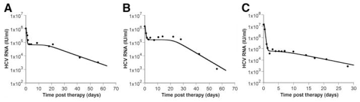
Even though a biphasic decline is the most commonly observed pattern in HCV viral kinetics, a triphasic decline with a shoulder phase separating the classic first and second phases (Fig. 2) has been reported in some patients treated with pegylated interferon-α plus ribavirin [49]. This pattern can be reproduced by models incorporating the proliferation of both uninfected and infected cells [50, 51].

Figure 2.

Shoulder phase. Patients treated with (A) pegylated IFN-α2a alone, (B) pegylated IFN-α2a plus RBV and (C) IFN-α2b alone sometimes show triphasic viral declines with a shoulder phase separating the rapid first phase and slower second or final phase. Viral load measurements are depicted by the filed circles, whereas the solid line is the best-fit of the model given by Eq. (4). Further details are given in [50]. Figure reproduced from [50] with permission of the publisher.

One such model including cell proliferation is [50]

$$\begin{array}{l}\frac{dT}{dt}=s+r_{T}T\left(1-\frac{T+1}{T_{max}}\right)-dT-(1-\eta )\beta TV\\ \frac{dI}{dt}=(1-\eta )\beta TV+r_{I}I\left(1-\frac{T+1}{T_{max}}\right)-\delta I\\ \frac{dV}{dt}=(1-\epsilon )pI-cV\end{array}$$ (4)

where r_T and r_I are the maximum proliferation rates of target cells and infected cells, respectively, and T_max is the maximum density of cells that the liver can reach. In order to have shoulder phase in which the viral load does not decline, the rate of de novo infection plus the rate of infected cell proliferation must equal the rate of infected cell lose. When this condition is met, the infected cell level and hence the viral load stays constant. However, if target cells proliferate faster than infected cells, which seems reasonable given that infection places a burden on the cell, then target cell levels will increase, which due to the density-dependent form of infected cell proliferation, will slow the rate of infected cell proliferation. This, in turn, will cause the critical balance needed to maintain the shoulder to be lost and viral loads will ultimately decline. A recent in vitro study suggests that HCV infected cells do in fact proliferate slower than infected cells and may even undergo cell cycle arrest [49]. Consistent with this, some models when used to fit in vivo data have found the proliferation of infected cells can be ignored [52].

Interestingly, while triphasic declines have been reported for patients treated with IFN and IFN plus ribavirin (RBV) [49], they have not been reported for patients treated with more potent regimes that include direct-acting antiviral agents (DAAs). The reason for this is not clear.

Critical drug efficacy

Most models of viral infection, including those given by Eqs. (1) and (4), predict that during therapy the viral load declines leading either to complete viral eradication (cure) or to a new on-therapy steady state with persistent viral infection.

Using Eq. (1) with target cell levels allowed to vary with time, Dahari et al. introduced the notion of a critical drug efficacy, ε_c, for the treatment of HCV [51]. They show that when the overall effectiveness of therapy, ε_tot = 1−(1−η)(1−ε) is greater than critical efficacy, ${\epsilon }_c=1-\frac{dc\delta }{sp\beta }$, the model predicts continuous viral decay and thus complete viral eradication. On the other hand, if ε_tot < ε_c, then the model predicts that HCV RNA levels will stabilize after an initial decline and will reach a new steady state despite continued therapy.

Describing the drug effect

The effectiveness of interferon treatment was initially modeled either as a constant 1-η multiplying the infectivity rate constant, and/or a constant 1-ε multiplying the virus production rate [6].

To model different drug dose regimens, one can include the dose as a covariate in the model [45]. However, the number of extra parameters to be estimated tends to grow considerably with the inclusion of such covariates. Another way to proceed is to include the dose in the effectiveness expression, e.g., $\epsilon =\frac{\mathit{Dose}}{{ED}_{50}+\mathit{Dose}}$, where ED₅₀ is the dose leading to 50% of the maximal effectiveness for this drug [38].

Drug effectiveness most realistically varies in time as the result of drug concentration changes. The observed fluctuations in effectiveness can be captured using a model that directly incorporates drug pharmacokinetics and pharmacodynamics [53–58]. Powers et al. and Talal et al. proposed a pharmacokinetic / viral kinetic (PK/VK) model to describe the viral kinetics for patients treated with pegylated interferon (PEG-IFN) once weekly with ribavirin for one or two weeks [56, 58]. The authors used a standard 1-compartment pharmacokinetic model for PEG-IFN α-2b. The most commonly used pharmacodynamic model is the Emax model [59]. A version of the Emax model was used to describe the relation between the PEG-IFN drug effectiveness and drug concentration, where the maximum effectiveness was set to 1 and a delay, τ, was introduced to account for the fact that IFN works by binding to cellular receptors and causing the upregulation of hundreds of cellular genes, processes that are assumed to take time τ. Thus, in modeling PEG-IFN the following effectiveness function was used: $\epsilon (t)=\frac{C{(t-\tau )}^h}{{EC}_{50}^h+C{(t-\tau )}^h}$ for t > τ and ε(t) = 0 for t < τ [56, 58].

By taking into account PEG-IFN pharmacokinetics, the authors could explain the early HCV RNA decays observed in HIV-HCV co-infected patients, followed by viral load increases as the drug concentration and efficacy decline between doses [56, 58]. They were also able to estimate the drug EC₅₀ in individual patients, and found, not surprisingly, that patients with low EC₅₀’s tended to respond to therapy and achieve a sustained virologic response, while patients with high EC₅₀’s tended to be non-responders to therapy [56].

Rather than dealing with a full PK model, which requires frequent drug concentration measurements in patients on therapy, changes in the drug effectiveness over time have been modeled phenomenologically [55, 60–62]. For a number of drugs the concentration of the drug increases with multiple doses until a steady state is reached. The effect of such increases have been modeled using the exponential function

$$\epsilon (t)={\epsilon }_1+\left({\epsilon }_2-{\epsilon }_1\right)\left(1-e^{kt}\right),$$ (5)

where ε₁ is the initial effectiveness, ε₂ is the final effectiveness and k is the transition rate from ε₁ to ε₂ [60, 61]. Using this function, Guedj et al. [60] showed that the progressive increase of effectiveness of the HCV nucleoside polymerase inhibitor mericitabine can explain the slow viral decline observed in some patients after they are first put on therapy. It was assumed that this progressive effectiveness increase is related to the requirement that mericitabine be triphosphorylated intracellularly in order to become effective [60].

Viral kinetic models in which the drug effectiveness increases with time have been called varying effectiveness (VE) models. The VE model given by Eqs. (1) and (5) has been recently solved analytically for a constant number of target cells, yielding (Conway and Perelson, submitted)

$$V(t)=\frac{e^{-(c+\delta )t/2}}{c\delta (1-\eta )}\left\{c_1\left[\left(\frac{\delta -c-k\nu }{2}\right)I_{\nu }(x(t))-\frac{kx(t)}{2}{I}_{\nu +1}(x(t))\right]+c_2\left[-\frac{c+\delta +k\nu }{2}\right]K_{\nu }(x(t))+\frac{kx(t)}{2}{K}_{\nu +1}(x(t))\right\}$$

where $\nu =\sqrt{{(c+\delta )}^2-4c\delta ({\epsilon }_{max}+(1-{\epsilon }_{max})\eta /k)},x(t)=2\sqrt{c\delta {\epsilon }_{max}(1-\eta )}{e}^{-kt/2}/k$, and I_ν and K_ν are modified Bessel function of the first- and second-kind of order ν.

A VE model using a Hill function, $\epsilon (t)={\epsilon }_{max}\frac{t^h}{{t_{50}}^h+t^h}$, where t₅₀ is the time necessary to reach 50% of the maximal effectiveness and h is a Hill coefficient characterizing the shape of the pharmacodynamic curve, has also has been proposed as a way to model the increase of antiviral effectiveness with time [63]. This effectiveness function was used to model the effect of therapy with two nucleotide analogues, sofosbuvir (GS-7977) and GS-0938, and proved to perform better than the exponential time-varying effectiveness model given by Eq. (5) [63]. Further, the effectiveness of using the combination of sofosbuvir and GS-038 was examined and it was found that a model in which the effectiveness of the two compounds were Loewe additive [64], i.e., $\epsilon =\frac{\frac{\mathrm{\epsilon }1}{1-\mathrm{\epsilon }1}+\frac{\mathrm{\epsilon }2}{1-\mathrm{\epsilon }2}}{1+\frac{\mathrm{\epsilon }1}{1-\mathrm{\epsilon }1}+\frac{\mathrm{\epsilon }2}{1-\mathrm{\epsilon }2}}$, fit the viral decline data better than a model in which the drugs were assumed to act independently yielding an ε given by (1 − ε)=(1−ε₁)(1−ε₂), where ε₁ and ε₂ are the effectiveness of sofosbuvir and GS-0938, respectively [63].

Modeling drug resistance

HCV, as other RNA viruses, has a high mutation rate, recently estimated as 2.5 × 10⁻⁵ per base per generation in vivo [65], and rapid replication cycles which lead to its rapid adaptation to selective pressures such as antiviral treatment [66]. One can therefore wonder if resistant viruses are present in the drug-naïve virus population before therapy or if they emerge during the treatment? If so, what is the probability of obtaining a mutant during treatment? What role does treatment selective pressure play? How should decreased viral fitness be taken into account?

Rong et al. [52] showed, for a conservative base substitution rate of μ=10⁻⁵, that the probability of 0, 1 and 2 mutations in an HCV genome occurring in a replication cycle is 91%, 8.7% and 0.42%, respectively. If we suppose that an infected patient typically produces 10¹² virions/day [6], approximately 8.7×10¹⁰ and 4.2×10⁹ mutants with single and double-nucleotide changes, respectively, will be generated each day. As the HCV genome contains ~9600 bases and each base can mutate to one of three possible different bases there are only 3 × 9600 ~ 2.9 ×10⁴ different single base substitutions and 4.1 × 10⁸ different pairs of substitutions. Thus, all possible single and double mutants are expected to be produced each day and most likely would be present at low frequencies prior to treatment [52]. The exact frequency would depend on the substitution rate and the fitness of the drug resistant variant in the absence of therapy [52]. However, in the presence of selective pressure applied by drug therapy, which can rapidly eliminate drug-sensitive virus, the existence of these variants, even at low levels can be revealed, which may explain why patients treated with a single antiviral drug with a low barrier to resistance can show a large proportion of resistant virus early after treatment initiation [52, 67].

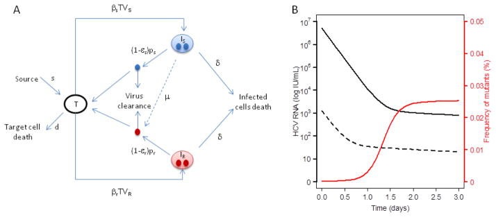
The following model (Fig. 3) can depict the dynamic of both drug-sensitive and drug-resistant virus in the absence of treatment [68]:

$$\begin{array}{l}\frac{dT}{dt}=s-dT-{\beta }_s{V}_{s}T-{\beta }_r{V}_{r}T\\ \frac{{dI}_s}{dt}={\beta }_s{V}_{s}T-\delta I_s\\ \frac{{dI}_r}{dt}={\beta }_r{V}_{r}T-\delta I_r\\ \frac{{dV}_s}{dt}=(1-\mu )p_s{I}_s-{cV}_s\\ \frac{{dV}_r}{dt}=\mu p_s{I}_s+p_r{I}_r-{cV}_r\end{array}$$ (6)

where I_s, I_r, V_s, and V_r are the number of cells infected with drug-sensitive virus, drug-resistant virus, free drug-sensitive virus, and free drug-resistant virus, respectively. Cells become infected with drug-sensitive virus at rate β_s and with drug-resistant virus at rate β_r. HCV virions are produced at rates, p_s and p_r, by infected cells I_s and I_r, while the two viral strains have the same viral clearance rate, c. It is assumed that cells infected with a drug-sensitive virus, I_s, produce drug-resistant virus with probability μ.

Figure 3. Modeling drug resistance.

(A) Schematic of the model for HCV infection with drug resistance where I_s, I_r, V_s, and V_r are the number of cells infected with drug-sensitive virus, drug-resistant virus, free drug-sensitive virus, and free drug-resistant virus, respectively. Cells become infected with drug-sensitive virus at rate β_s and with drug-resistant virus at rate β_r. HCV virions are produced at rates, p_s and p_r, by infected cells I_s and I_r. The two viral strains are assumed to have the same viral clearance rate, c. It is also assumed that cells infected with a drug-sensitive virus, I_s, produce drug-resistant virus with probability μ. (B) Simulation of drug-sensitive and drug-resistant viral load kinetics with a mutation rate μ=10⁻⁴ and effectivenesses ε_s=0.9997 and ε_r=0.95 against the drug-sensitive and drug-resistant viral strains respectiviely. The infectivity rate constant β, is 10⁻⁷ mL day⁻¹ virions⁻¹ for both strains, the virus production rate for the drug-sensitive strain is 10 virions cell⁻¹ day⁻¹ and 6 virions cell⁻¹ day⁻¹ for the drug-resistant strain.

When measurement for the kinetics of several known variants is available, for instance by clonal sequencing, a more comprehensive picture of viral competition can be obtained with a model including the various viral variants [68, 69]. For example, Rong et al. [68] constructed a model that considered substitutions occurring at four positions in the HCV protease gene that had previously been identified with drug resistance to the protease inhibitor telaprevir. The full model without considering backward mutations is given by:

$$\begin{array}{l}\frac{d}{dt}T(t)=s-dT-\sum _j{\beta }_j{V}_j\\ \frac{d}{dt}{I}_j(t)=\sum _j{\beta }_j{V}_j-\delta I_j\\ \frac{d}{dt}{V}_0(t)={(1-\mu )}^4{p}_0{I}_0-{cV}_0\\ \frac{d}{dt}{V}_i(t)=\mu {(1-\mu )}^3{p}_0{I}_0+{(1-\mu )}^3{p}_i{I}_i-{cV}_i,i=1,2,3,4\\ \frac{d}{dt}{V}_{ij}(t)={\mu }^2{(1-\mu )}^2{p}_0{I}_0+\mu {(1-\mu )}^2\left(p_i{I}_i+p_j{I}_j\right)+{(1-\mu )}^2{p}_{ij}{I}_{ij}-{cV}_{ij},i,j=1,2,3,4\text{and}i<j\\ \frac{d}{dt}{V}_{\mathit{ijk}}(t)={\mu }^3(1-\mu )p_0{I}_0+{\mu }^2(1-\mu )\left(p_i{I}_i+p_j{I}_j+p_k{I}_k\right)+\mu (1-\mu )\left(p_{ij}{I}_{ij}+p_{ik}{I}_{ik}+p_{jk}{I}_{jk}\right)\\ +(1-\mu )p_{\mathit{ijk}}{I}_{\mathit{ijk}}-{cV}_{\mathit{ijk}},i,j,k=1,2,3,4\text{and}i<j<k\\ \frac{d}{dt}{V}_{1234}(t)={\mu }^4{p}_0{I}_0+{\mu }^3\sum _{i=1}^4{p}_i{I}_i+{\mu }^2\sum _{\begin{array}{c}i,j=1,2,3,4\\ i<j\end{array}}{p}_{ij}{I}_{ij}+\mu \sum _{\begin{array}{c}i,j,k=1,2,3,4\\ i<j<k\end{array}}{p}_{\mathit{ijk}}{I}_{\mathit{ijk}}+p_{1234}{I}_{1234}-{cV}_{1234}\end{array}$$

In the first two equations, the strain index j is in the set Ω = {0,1,2,3,4,12,13,14,23,24,34,123,124,134,234,1234}. Strain 0 represents wild-type virus; strains 1, 2, 3, 4 represent the viral strains with mutations occurring at positions 36, 54, 155, and 156, respectively, where drug resistant mutations are commonly found in protease. Strains ij, with i, j = 1,2,3,4 and i < j, are the strains with double mutations occurring at positions i and j. Strains ijk, with i, j, k = 1,2,3,4 and i < j < k, and strain 1234 can be defined similarly. In this model, there is conservation of viruses as they mutate within the self-contained system of 16 strains [68].

Adiwijaya et al. [69] estimated the in vivo fitness of the principal single and double mutants observed during two weeks of monotherapy with the HCV protease inhibitor telaprevir. The authors then applied their model to various phase 2/3 studies where telaprevir was given in combination with peg-IFN/RBV for longer times [57]. This model was used to predict the observed SVR rates for various regimens and suggested that modeling might be a relevant approach to design treatment strategies.

Multiscale modeling

The standard HCV model has been extended [70–72] to describe the intracellular processes that are targeted by drugs such as direct acting antivirals. In this model, the level of intracellular viral RNA (vRNA, denoted R) depends on the time since the cell has been infected (denoted a) and can be modeled as:

$$\frac{dR}{da}=(1-{\epsilon }_a)\alpha -\kappa \mu R-(1-{\epsilon }_s)\rho R,$$ (7)

where α, μ and ρ are the intracellular rate of vRNA production, degradation and assembly/secretion, respectively. In this model, treatment can act in three different possible ways: 1) by blocking intracellular viral production with efficacy ε_α, 2) by blocking virion assembly and/or secretion with effectiveness ε_s and 3) by increasing the degradation rate of vRNA by a factor κ. We can therefore write the full model combining the intracellular and extracellular dynamic as:

$$\begin{array}{l}\frac{dT}{dt}=s-dT-\beta TV\\ \frac{\partial I}{\partial a}+\frac{\partial I}{\partial t}=-\delta I(a,t)\\ \frac{\partial R}{\partial a}+\frac{\partial R}{\partial t}=(1-{\epsilon }_{\alpha })\alpha -\kappa \mu R-(1-{\epsilon }_s)\rho R\\ \frac{dV}{dt}=(1-{\epsilon }_s)\rho \underset{0}{\overset{\infty }{\int }}R(a,t)I(a,t)da-cV,\end{array}$$ (8)

with boundary conditions and initial conditions I(0,t) = βVT, I(a,0) = I₀(a), R(0,t) = 1, R(a,0) = R₀(a), where I₀(a) and R₀(a) are the pre-treatment steady-state distributions representing the number of infected cells of age a and the vRNA levels within cells of age a. Note that the rate of viral production from an infected cell depends on the amount of intracellular vRNA that cell contains. In this model that dependence is linear, but extensions using a nonlinear dependence are straightforward. Under the assumption that treatment is potent enough that the number of new cell infections after treatment initiation is negligible, which can be translated as I(a,t) = 0 for a < t, this model can be solved and yields [71, 72]

$$V(t)=V_0\left\{e^{-c(t-t_0)}+\frac{\stackrel{\sim }{\rho }c}{N}\left[\frac{\stackrel{\sim }{\alpha }}{\stackrel{\sim }{\lambda }\delta (\delta -c)}\left(e^{-c(t-t_0)}-e^{-\delta (t-t_0)}\right)+\frac{1}{\stackrel{\sim }{\lambda }+\delta -c}\left(\frac{N}{\rho }-\frac{\stackrel{\sim }{\alpha }}{\stackrel{\sim }{\lambda }\delta }\right)\left(e^{-c(t-t_0)}-e^{-(\stackrel{\sim }{\lambda }+\delta )(t-t_0)}\right)\right]\right\}$$ (8)

for a pharmacologic lag-time t₀ before the viral load decline begins, α̃ = α(1 − ε_α), ρ̃ = ρ(1 − ε_s), λ̃ = ρ̃ + κμ and $N=\rho \frac{\alpha +\delta }{\delta (\rho +\mu +\delta )}.$.

Multiscale models add realism in that they can account for steps in the viral lifecycle affected by a drug. For example, in the case of the NS5A inhibitor daclatasvir, Guedj et al. [70] showed that the drug had two modes of action: reducing vRNA production and reducing viral assembly or secretion. Further, in these models the rate of virus production from a cell is not constant and when a cell is first infected essentially no virus is produced until vRNA is replicated. Thus these models allow the rate of virus production to depend on the age of an infected cell. The models can also allow the death rate of an infected cell to depend on its age or the amount of vRNA they contain. Other formulations of multiscale models are also possible. For example, rather than using partial differential equations, one can use a system of ordinary differential equations in which one introduces variables to represent infected cells containing i vRNA molecules, i=1,2,…n. This has the disadvantage of having to specify a maximum number of vRNAs per cell, but has the advantage of having the vRNA content being an integer and allowing one to introduce models with a threshold such that only cells with more than a threshold number of vRNAs encapsidate vRNA into virions, whereas cells with less than this threshold only replicate vRNA (Rong and Perelson, unpublished).

Cell-to-cell spread

Hepatitis C is an infection of a solid tissue and as such the focal release of virus from infected cells may have important effects on viral kinetics. Examination of biopsy samples has revealed that infected cells tend to be found in clusters [73], consistent with a model where infections are randomly seeded and then spread locally [Graw et al., submitted]. If we consider that the virus most likely preferentially infects nearby cells, the models presented above, which assume a well-mixed system with virus equally likely to infect any cell, cannot describe this spatial localization of infection. Further, infection can spread either through virus being released from an infected cell and infecting another cell or by direct cell-to-cell transmission. The models presented above do not consider the possibility of cell-to-cell transmission. Several methods are available to include spatial aspects into the modeling of viral infections. These have recently been reviewed in the context of HIV infection [74] and in the context of agent-based models of host-pathogen systems including influenza [75] and hence will not be discussed here. Explicit models for the spatial spread of HCV are under development but to our knowledge none have been published.

Influenza viral kinetics modeling

Influenza viral kinetics has received increasing attention over the last decade. As an acute infection, the viral shedding period is short and a number of adaptations are necessary. First, considering the short duration of influenza, target cell production and death can be ignored. Second, an eclipse phase in the infected cells dynamic was included assuming that infected cells do not die before they begin to produce viruses. Baccam et al. [21] described influenza infection with the following model (Fig. 4a):

$$\begin{array}{l}\frac{dT}{dt}=-\beta TV\\ \frac{{dI}_1}{dt}=\beta TV-{kI}_1\\ \frac{{dI}_2}{dt}={kI}_1-\delta I_2\\ \frac{dV}{dt}={pI}_2-cV\end{array}$$

where T is the number of epithelial target cells, I₁ the number of infected cells not producing virus (eclipse phase), I₂ the number of productively infected cells and V the free virus shed. The model assumes that the virus infects target cells at rate β, the non-productive infected cells move to the productive stage at rate k, the productively infected cells die at rate δ and produce virus at rate p, and the virus is cleared at rate c [21].

Figure 4. Mathematical modeling of influenza kinetics.

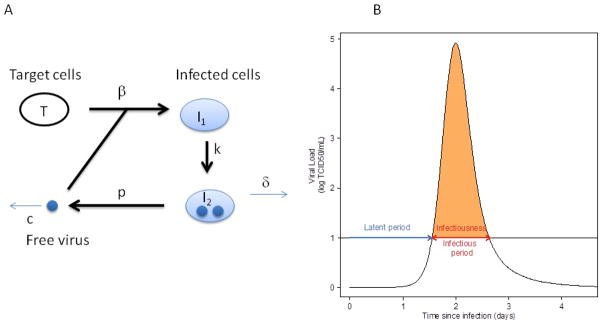
(A) Schematic of the model for influenza infection by Baccam et al. [21] as described in the text. In this model, target cells, T, are infected with rate constant β and generate infected cells, I₁, that are infected but not yet producing virus, i.e. are in the eclipse phase of infection. These cells transition at rate k into infected cell, I₂, that produce virus at rate p per cell, which is then cleared at rate c per virion. (B) Example of influenza infection viral load curve and definition of the epidemiological parameters depending on the threshold between the noninfectious and infectious state. Here the threshold is denoted by the black horizontal line at 10 TCID₅₀/ml. As discussed in the text, the infectiousness is the area under the viral load curve that is above threshold, depicted in orange. The infectious period is the time interval the viral load is above threshold and is also indicated

Baccam et al. [21] also computed the basic reproductive number, $R_0=\frac{p\beta T_0}{c\delta }$, which represents the average number of secondary infections produced by a single infected cell placed in a population of entirely susceptible cells, where T₀ is the initial number of target cells. For experimental infection of humans using an H1N1 virus for which the subjects were all seronegative, R₀ was estimated as 22. This high value suggests that the initial infection could spread rapidly within the respiratory tract and is consistent with virus titer reaching a peak at 2 days post-infection [21].

It is also possible to compute epidemiological parameters from within-host viral kinetics. In the epidemiological literature, viral load has been used as a surrogate for the infectiousness of an individual [76–78], where the viral load must be above a given threshold for a person to be infectious (Fig. 4b). How infectious a person is, their infectiousness, has been defined as the area between the viral load curve as computed from a viral kinetic model and the threshold [24]. Initially, the viral load is below this threshold and a person is considered to be non-infectious and in the latent period of the infection. During infection the viral load curve may cross the threshold and then the duration of infectiousness is defined as the period during which the viral load is above this threshold [24].

Innate immune control

In addition to viral cytopathic effects, modeled by the loss of infected cells at rate δ, innate immune responses can also affect viral kinetics. Type I interferon (IFN) is a significant component of the innate response. A model proposed for the innate immune response to influenza infection was an extension of the previous one which described the IFN kinetics as $\frac{dF}{dt}={sI}_2(t-\tau )-\alpha F$, where F is the IFN level, s is the rate at which IFN is secreted by virus-producing cells, τ is the lag-time necessary for the virus-producing cells to begin secreting IFN and α is the IFN clearance rate [21]. The effect of interferon was modeled as a decrease of the virus production rate, $p=\frac{\widehat{p}}{1+{\epsilon }_{p}F}$, and/or as a decrease of the rate at which nonproductive cells move into the virus-producing state, $k=\frac{\widehat{k}}{1+{\epsilon }_{k}F}$, where p̂ and k̂ are the value of these parameters in the absence of IFN and ε_p and ε_k represent the IFN effectiveness [21]. Another way to describe IFN’s effect is to assume that IFN creates an antiviral state within uninfected cells that prevents their infection. This has been modeled by allowing target cells to move into a compartment of cells that are refractory to infection at rate proportional to the IFN concentration [25, 28, 29].

Another component of the innate immune response is the cytotoxic effect of natural killer (NK) cells. Canini and Carrat [24] proposed a model where NK cells activation is stimulated by pro-inflammatory cytokines, such as IFN, and the dynamics of activated NK cells obey the equation $\frac{dN}{dt}=F-\xi N$, where ξ is the activated NK cell death rate. In their model, NK cells increase the death rate of productively infected cells, so that $\frac{{dI}_2}{dt}={kI}_1-\delta I_2-\eta I_{2}N$. The model was used to fit data from 44 experimentally influenza infected volunteers and predicted that NK cell levels peak around day 4 after infection and then decay slowly, whereas pro-inflammatory cytokines peak at 2.2 days after infection and have a short half-life of 9.1 hr [24]. These results were recently confirmed by experiments showing that NK cell activation peaks between 3 and 5 days after infection [79, 80]. Also, if one assumes that the level of activated NK cells rapidly reaches a steady state, then by a quasi-steady state assumption N is proportional to the inflammatory cytokine level, F. Pawelek et al. [28] used this assumption in a model of equine influenza infection and showed that such a model could simultaneously fit data on viral titers and interferon levels.

Adaptive immune control

In addition to innate immune responses, adaptive immune responses involving cytotoxic T lymphocytes, CTLs, and specific antibodies and their role in influenza virus clearance have been modeled [26, 27, 81, 82]. However, in experiments involving influenza infection of humans, subjects are generally naïve to infection. Thus, the effect of preexisting immunity on influenza infection dynamics in humans remains unstudied. However, immune functions decline due to aging, a phenomenon called immunosenescence [83], and this leads to influenza having more serious health consequences in the elderly. While not modeled in humans, a recent viral kinetic model analyzed the effect of aging on innate and adaptive immune responses in the context of influenza viral kinetics in mice [84].

Symptom dynamic

In the case of influenza infection, symptom scores can be easily collected by questionnaire. Pro-inflammatory cytokines have a protective role, but their levels also correlate with systemic symptom dynamics. In particular, IL-6 and IFN-α levels in nasal wash fluid are causally linked to viral titers, body temperature, mucus production, and symptom scores [85]. Canini and Carrat [24] included systemic symptom dynamics in an influenza viral dynamic model. They assumed $\frac{dS}{dt}=\gamma F-hS$, where S is the systemic symptom score, F is the concentration of proinflammatory cytokines, γ is the rate at which systemic symptoms appear and h is the rate of symptom resolution. Using this model they simultaneously fit viral kinetics and systemic symptom dynamics data. They described the dynamics of the systemic symptoms with a peak 2.5 days after infection or 0.5 day after the viral load peak. The incubation period, which is the period during which a subject is infected and asymptomatic [86], can be derived from the symptom dynamics (SD) curve. Based on this Canini and Carrat [24] predicted an incubation period of 1.9 days for healthy volunteers experimentally infected with H1N1 influenza in agreement with epidemiological studies [77].

Antiviral treatment

A model similar to the one used for protease inhibitors in HCV infection was used for neuraminidase inhibitor treatment for influenza, where it was assumed the drug reduced viral production from infected cells [21, 87]. More recently, in order to model the generation of drug resistant variants during influenza infection and treatment, a hybrid deterministic-stochastic approach has been used [88]. In this work, both influenza viral kinetics and symptom dynamics were simulated for subjects treated with the neuraminidase inhibitor oseltamivir in order to assess the virological and symptom efficacy of oseltamivir as well as the risk of resistance emergence depending on the treatment initiation time, dose, intake frequency and duration of treatment [88]. This study, which also incorporated the pharmacokinetics of oseltamivir, showed that initiating oseltamivir treatment during the incubation period increases the risk of drug-resistant virus emergence. Based on their results, the authors recommended that oseltamivir prophylaxis should be restricted either to subjects prone to developing severe cases (such as immunocompromised subjects), who should be treated with high doses, frequent intakes and for longer duration than usual, or in otherwise healthy patients, after exclusion of an influenza infection in the incubation period, in order to decrease the risk of resistant virus emergence and to preserve oseltamivir efficacy [88].

In order to identify new drug targets, a multiscale model has been develop for influenza infection comprising both the intracellular level, where the virus synthesizes its proteins, replicates its genome, and assembles new virions, and the extracellular level where the virus spreads to new target cells [89]. The authors suggest that inhibitors of viral transcription, replication, protein synthesis, nuclear export, and assembly/release are most effective in decreasing virus titers, whereas targeting virus entry primarily delays infection.

Conclusions

Viral kinetic modeling has led to several important insights about the dynamics and pathogenesis of infectious diseases. Modeling plasma virus decay for HCV under therapy demonstrated the fast turnover of virus, explaining the potential for generation of mutants and the development of drug resistance. It also allowed evaluation of the in vivo effectiveness of drugs in clinical development using short clinical trials, as models showed that the effectiveness in blocking viral production could be estimated from the magnitude of the first phase viral decline after the initiation of therapy [6, 60, 63, 70, 90]. Many insights were the result of close interdisciplinary collaborations between modelers and clinicians who obtained and made available frequently collected viral kinetic data.

Mathematical modeling of viral kinetics continues to provide biologically plausible explanations of viral kinetic data obtained from patients under therapy. For HCV, the objective of therapy is to reach sustained virologic response rates approaching 100%, while reducing the duration of treatment and eliminating the use of IFN and ribavirin. To achieve this goal, several combinations of direct acting antivirals (DAA) are currently being evaluated in clinical trials. Mathematical modeling may offer an appropriate tool to investigate and optimize different drug combinations and dosing regimens. For example, as discussed above, Guedj et al. [63] analyzed the kinetics of viral decline during monotherapy with the HCV polymerase inhibitors sofosbuvir and GS-0938 as well as during combination therapy using these two agents in the same patients with a crossover design in which a single agent was given for one week followed by the addition of the second agent for a week. Their analysis showed that the drug effects exhibited Lowe additivity [64]. For other drug combinations, such as Peg-IFN and telaprevir, the drug effects seem multiplicative, i.e. the effectiveness of the combination obeys the equation (1−ε)=(1−ε₁)(1−ε₂), where ε₁ and ε₂ are the effectiveness of Peg-IFN and telaprevir, respectively [68, 91]. As we go forward it will be critical to determine how the effectiveness of drug combinations compares with that of the single agents being combined.

Another major outstanding problem is to determine the needed duration of therapy. This is being done empirically, but theory can help guide such studies. For example, Guedj et al. analyzed the viral decline kinetics of 44 patients treated with telaprevir. Based on the distribution of viral kinetic parameters found using a population fitting approach they then created an in silico population of 10,000 patients and computed the cumulative distribution function of the time to eliminate the last viral particle or last infected cell. From their analysis they suggested that combination therapy in which resistance was not an issue and which is as potent as that observed during short-term telaprevir treatment could lead to SVR in 95% of patients after 7 weeks of therapy, and that some patients might be cured in as little as 3 or 4 weeks [90]. A recent case report confirmed this prediction by showing that a patient treated with the HCV polymerase inhibitor sofosbuvir plus ribavirin attained SVR after 27 days of therapy [see attached preprint]. Also, the SYNERGY trial showed that 39 out of 40 patients treated with three direct acting antivirals for 6 weeks attained SVR, again confirming the prediction that potent combination therapy could be given for short periods and cure a large fraction of patients [92]. How to identify the drug combinations that can lead to short-term cure and the patients that can attain SVR with short duration therapy is a pressing question. With drugs such as sofosbuvir costing $1000 a pill, economic issues will also play an important role in determining HCV treatments as we move forward.

For both influenza and HCV, the determinants of physiopathology and the role of the different components of the immune response in both protection and in the potential generation of immunopathology have not been completely elucidated. As more quantitative data on the immune response, both innate and adaptive, become available, it will be important to include these in mechanistic viral kinetic models. Understanding the within-host dynamics of influenza infection will bring invaluable information on the between-host dynamics and how to mitigate its spread in the population.

Although standard viral dynamic models brought valuable insights into the origin of viral declines observed during treatment for HCV with high daily doses of standard IFN [6], and into the within-host dynamics of influenza [21], the model extensions presented in this review that involve including drug pharmacokinetics or time-varying drug effectiveness are needed to understand the subtleties of viral kinetics patterns under different treatments. The viral kinetic models developed recently also rely on detailed biological knowledge. For example, multiscale models for HCV that include the intracellular dynamics of the virus, suggested that the HCV NS5A inhibitor daclatasvir has two modes of action, one of which reduces vRNA production and the other which inhibits viral assembly or secretion [70]. In vitro experiment’s then validated these predictions [70].

Current HCV models have all been built using measurements of plasma viral load. The dynamics of target cells and infected cells generally are inferred. Analysis of biopsy samples suggest that infected cells lie in clusters [73, 93] and that only a fraction of cells in the biopsy samples are infected. Future models need to address the spatial distribution of infection within the liver, address whether viral spread in the liver is by cell-free virus infecting target cells as in the standard models or whether it also occurs by direct cell-to-cell infection, and determine whether these issues matter when evaluating a patient’s response to therapy.

The SYNERGY trial mentioned above also had another surprising finding. At the end of treatment nearly half of the 60 patients had detectable viremia when an Abbott real-time PCR assay was used and yet only one of these patients failed to attain SVR [94]. Existing theory would predict that when therapy was withdrawn virus would rebound in these patients, as has been seen in all monotherapy studies. Clearly, theory needs to be revised and the biological basis of these observations needs to be understood.

Concerning influenza, one important challenge lies in data collection for naturally acquired infections. One study prospectively followed-up index cases and their household contacts during the summer of 2009 in Hong Kong [95]. Viral loads were measured in all household members at three home visits within 7 days of index case diagnosis. This study provided the first data characterizing the time course of the 2009 pandemic influenza infection. However, due to the unknown infection date and sparse sample collection, the viral load peak could not be identified and this data could not be fitted with a viral kinetic model.

An optimal design approach, based on the maximization of the Fisher information matrix [96], has been used to provide designs for studying influenza viral kinetics following experimental infection and showed that 20 subjects and 5 sample times per subject were necessary to accurately estimate viral kinetic parameters [97]. Efforts are needed to developed ready-to-use study designs that could be implemented for naturally acquired infection in the general population.

Modeling respiratory symptoms dynamics would be of great interest. Indeed, Gustin et al. showed that the number of infectious particles produced during sneezing is twice that produced by normal breathing [98]. However, the underlying physiological mechanisms for respiratory symptoms such as sneezing and coughing are complex. They are related to local inflammation at different sites, such as the nasopharynx, larynx and the lower respiratory tract [99]. Taking into account respiratory symptom dynamics in estimating a person’s infectiousness could change estimates of epidemiological parameters and could help understanding the routes of transmission of influenza infection.

In the future, we expect to see more detailed models, integrating the influence of both viral and host factors and the effects of therapy, which have the potential to deepen our understanding of infectious diseases. We also foresee the development of viral kinetic models for other infections and the expansion of such techniques into the realm of bacterial and fungal infections and treatment.

References

- 1.Ho DD, et al. Rapid turnover of plasma virions and CD4 lymphocytes in HIV-1 infection. Nature. 1995;373(6510):123–126. doi: 10.1038/373123a0. [DOI] [PubMed] [Google Scholar]
- 2.Perelson AS. Modelling viral and immune system dynamics. Nature Rev Immunol. 2002;2(1):28–36. doi: 10.1038/nri700. [DOI] [PubMed] [Google Scholar]
- 3.Perelson AS, et al. Decay characteristics of HIV-1-infected compartments during combination therapy. 1997 doi: 10.1038/387188a0. [DOI] [PubMed] [Google Scholar]
- 4.Perelson AS, et al. HIV-1 dynamics in vivo: virion clearance rate, infected cell life-span, and viral generation time. Science. 1996;271(5255):1582–1586. doi: 10.1126/science.271.5255.1582. [DOI] [PubMed] [Google Scholar]
- 5.Wei X, et al. Viral dynamics in human immunodeficiency virus type 1 infection. Nature. 1995;373(6510):117–122. doi: 10.1038/373117a0. [DOI] [PubMed] [Google Scholar]
- 6.Neumann AU, et al. Hepatitis C viral dynamics in vivo and the antiviral efficacy of interferon-alpha therapy. Science. 1998;282(5386):103–107. doi: 10.1126/science.282.5386.103. [DOI] [PubMed] [Google Scholar]
- 7.Ciupe SM, et al. The role of cells refractory to productive infection in acute hepatitis B viral dynamics. Proc Natl Acad Sci U S A. 2007;104(12):5050–5055. doi: 10.1073/pnas.0603626104. [DOI] [PMC free article] [PubMed] [Google Scholar]
- 8.Ciupe SM, et al. Modeling the mechanisms of acute hepatitis B virus infection. J Theor Biol. 2007;247(1):23–35. doi: 10.1016/j.jtbi.2007.02.017. [DOI] [PMC free article] [PubMed] [Google Scholar]
- 9.Dahari H, et al. Modeling complex decay profiles of hepatitis B virus during antiviral therapy. Hepatology. 2009;49(1):32–38. doi: 10.1002/hep.22586. [DOI] [PMC free article] [PubMed] [Google Scholar]
- 10.Lewin SR, et al. Analysis of hepatitis B viral load decline under potent therapy: complex decay profiles observed. Hepatology. 2001;34(5):1012–1020. doi: 10.1053/jhep.2001.28509. [DOI] [PubMed] [Google Scholar]
- 11.Murray JM, et al. Dynamics of hepatitis B virus clearance in chimpanzees. Proc Natl Acad Sci U S A. 2005;102(49):17780–17785. doi: 10.1073/pnas.0508913102. [DOI] [PMC free article] [PubMed] [Google Scholar]
- 12.Nowak MA, et al. Viral dynamics in hepatitis B virus infection. Proc Natl Acad Sci U S A. 1996;93(9):4398–4402. doi: 10.1073/pnas.93.9.4398. [DOI] [PMC free article] [PubMed] [Google Scholar]
- 13.Ribeiro RM, et al. Hepatitis B virus kinetics under antiviral therapy sheds light on differences in hepatitis B e antigen positive and negative infections. J Infect Dis. 2010;202(9):1309–1318. doi: 10.1086/656528. [DOI] [PMC free article] [PubMed] [Google Scholar]
- 14.Ribeiro RM, Lo A, Perelson AS. Dynamics of hepatitis B virus infection. Microb Infect. 2002;4(8):829–835. doi: 10.1016/s1286-4579(02)01603-9. [DOI] [PubMed] [Google Scholar]
- 15.Emery VC, Griffiths PD. Prediction of cytomegalovirus load and resistance patterns after antiviral chemotherapy. Proc Natl Acad Sci U S A. 2000;97(14):8039–8044. doi: 10.1073/pnas.140123497. [DOI] [PMC free article] [PubMed] [Google Scholar]
- 16.Emery VC, et al. Differential decay kinetics of human cytomegalovirus glycoprotein B genotypes following antiviral chemotherapy. J Clin Virol. 2012;54(1):56–60. doi: 10.1016/j.jcv.2012.01.015. [DOI] [PMC free article] [PubMed] [Google Scholar]
- 17.Regoes RR, et al. Modelling cytomegalovirus replication patterns in the human host: factors important for pathogenesis. P Roy Soc B-Biol Sci. 2006;273(1596):1961–1967. doi: 10.1098/rspb.2006.3506. [DOI] [PMC free article] [PubMed] [Google Scholar]
- 18.Schiffer JT, Corey L. Rapid host immune response and viral dynamics in herpes simplex virus-2 infection. Nature Med. 2013;19(3):280–288. doi: 10.1038/nm.3103. [DOI] [PMC free article] [PubMed] [Google Scholar]
- 19.Schiffer JT, et al. Rapid localized spread and immunologic containment define Herpes simplex virus-2 reactivation in the human genital tract. Elife. 2013:2. doi: 10.7554/eLife.00288. [DOI] [PMC free article] [PubMed] [Google Scholar]
- 20.Schiffer JT, et al. The kinetics of mucosal herpes simplex virus–2 infection in humans: evidence for rapid viral-host interactions. J Infect Dis. 2011;204(4):554–561. doi: 10.1093/infdis/jir314. [DOI] [PMC free article] [PubMed] [Google Scholar]
- 21.Baccam P, et al. Kinetics of influenza A virus infection in humans. J Virol. 2006;80(15):7590–9. doi: 10.1128/JVI.01623-05. [DOI] [PMC free article] [PubMed] [Google Scholar]
- 22.Beauchemin C, Samuel J, Tuszynski J. A simple cellular automaton model for influenza A viral infections. J Theor Biol. 2005;232(2):223–34. doi: 10.1016/j.jtbi.2004.08.001. [DOI] [PubMed] [Google Scholar]
- 23.Bocharov GA, Romanyukha AA. Mathematical model of antiviral immune response. III. Influenza A virus infection. J Theor Biol. 1994;167(4):323–60. doi: 10.1006/jtbi.1994.1074. [DOI] [PubMed] [Google Scholar]
- 24.Canini L, Carrat F. Population modeling of influenza A/H1N1 virus kinetics and symptom dynamics. J Virol. 2011;85(6):2764–70. doi: 10.1128/JVI.01318-10. [DOI] [PMC free article] [PubMed] [Google Scholar]
- 25.Hancioglu B, Swigon D, Clermont G. A dynamical model of human immune response to influenza A virus infection. J Theor Biol. 2007;246(1):70–86. doi: 10.1016/j.jtbi.2006.12.015. [DOI] [PubMed] [Google Scholar]
- 26.Handel A, I, Longini M, Jr, Antia R. Towards a quantitative understanding of the within-host dynamics of influenza A infections. J R Soc Interface. 2010;7(42):35–47. doi: 10.1098/rsif.2009.0067. [DOI] [PMC free article] [PubMed] [Google Scholar]
- 27.Miao H, et al. Quantifying the early immune response and adaptive immune response kinetics in mice infected with influenza A virus. J Virol. 2010;84(13):6687–98. doi: 10.1128/JVI.00266-10. [DOI] [PMC free article] [PubMed] [Google Scholar]
- 28.Pawelek KA, et al. Modeling within-host dynamics of influenza virus infection including immune responses. PLoS Comput Biol. 2012;8(6):e1002588. doi: 10.1371/journal.pcbi.1002588. [DOI] [PMC free article] [PubMed] [Google Scholar]
- 29.Saenz RA, et al. Dynamics of influenza virus infection and pathology. J Virol. 2010;84(8):3974–83. doi: 10.1128/JVI.02078-09. [DOI] [PMC free article] [PubMed] [Google Scholar]
- 30.Smith AM, et al. Effect of 1918 PB1-F2 expression on influenza A virus infection kinetics. PLoS Comput Biol. 2011;7(2):e1001081. doi: 10.1371/journal.pcbi.1001081. [DOI] [PMC free article] [PubMed] [Google Scholar]
- 31.Smith AM, Perelson AS. Influenza A virus infection kinetics: quantitative data and models. Wiley Interdiscip Rev Syst Biol Med. 2011;3(4):429–445. doi: 10.1002/wsbm.129. [DOI] [PMC free article] [PubMed] [Google Scholar]
- 32.Perelson AS, Rong L, Hayden FG. Combination antiviral therapy for influenza: predictions from modeling of human infections. J Infect Dis. 2012;205(11):1642–1645. doi: 10.1093/infdis/jis265. [DOI] [PMC free article] [PubMed] [Google Scholar]
- 33.Murillo LN, Murillo MS, Perelson AS. Towards multiscale modeling of influenza infection. J Theor Biol. 2013;332:267–290. doi: 10.1016/j.jtbi.2013.03.024. [DOI] [PMC free article] [PubMed] [Google Scholar]
- 34.Smith AM, et al. Kinetics of coinfection with influenza A virus and Streptococcus pneumoniae. PLoS Pathog. 2013;9(3):e1003238. doi: 10.1371/journal.ppat.1003238. [DOI] [PMC free article] [PubMed] [Google Scholar]
- 35.Asquith B, Bangham CR. Quantifying HTLV-I dynamics. Immunol Cell Biol. 2007;85(4):280–286. doi: 10.1038/sj.icb.7100050. [DOI] [PubMed] [Google Scholar]
- 36.Heffernan J, Keeling MJ. An in-host model of acute infection: Measles as a case study. Theor Popul Biol. 2008;73(1):134–147. doi: 10.1016/j.tpb.2007.10.003. [DOI] [PubMed] [Google Scholar]
- 37.Zhang J, et al. Modeling the acute and chronic phases of Theiler murine encephalomyelitis virus infection. J Virol. 2013;87(7):4052–4059. doi: 10.1128/JVI.03395-12. [DOI] [PMC free article] [PubMed] [Google Scholar]
- 38.Snoeck E, et al. A comprehensive hepatitis C viral kinetic model explaining cure. Clin Pharmacol Ther. 2010;87(6):706–713. doi: 10.1038/clpt.2010.35. [DOI] [PubMed] [Google Scholar]
- 39.Guedj J, et al. Modeling viral kinetics and treatment outcome during alisporivir interferon-free treatment in HCV genotype 2/3 patients. Hepatology. doi: 10.1002/hep.26989. in press. [DOI] [PubMed] [Google Scholar]
- 40.Gao M, et al. Chemical genetics strategy identifies an HCV NS5A inhibitor with a potent clinical effect. Nature. 2010;465(7294):96–100. doi: 10.1038/nature08960. [DOI] [PMC free article] [PubMed] [Google Scholar]
- 41.Beauchemin CA, et al. Modeling amantadine treatment of influenza A virus in vitro. J Theor Biol. 2008;254(2):439–451. doi: 10.1016/j.jtbi.2008.05.031. [DOI] [PMC free article] [PubMed] [Google Scholar]
- 42.Bochud PY, et al. IL28B polymorphisms predict reduction of HCV RNA from the first day of therapy in chronic hepatitis C. J Hepatol. 2011;55(5):980–988. doi: 10.1016/j.jhep.2011.01.050. [DOI] [PubMed] [Google Scholar]
- 43.Dahari H, et al. Hepatitis C viral kinetics in the era of direct acting antiviral agents and interleukin-28B. Curr Hepat Rep. 2011;10(3):214–227. doi: 10.1007/s11901-011-0101-7. [DOI] [PMC free article] [PubMed] [Google Scholar]
- 44.Guedj H, et al. The impact of fibrosis and steatosis on early viral kinetics in HCV genotype 1–infected patients treated with Peg-IFN-alfa-2a and ribavirin. J Viral Hepat. 2012;19(7):488–496. doi: 10.1111/j.1365-2893.2011.01569.x. [DOI] [PubMed] [Google Scholar]
- 45.Guedj J, et al. Understanding silibinin’s modes of action against HCV using viral kinetic modeling. J Hepatol. 2012;56(5):1019–24. doi: 10.1016/j.jhep.2011.12.012. [DOI] [PMC free article] [PubMed] [Google Scholar]
- 46.Lagging M, et al. Response prediction in chronic hepatitis C by assessment of IP-10 and IL28B-related single nucleotide polymorphisms. PLoS One. 2011;6(2):e17232. doi: 10.1371/journal.pone.0017232. [DOI] [PMC free article] [PubMed] [Google Scholar]
- 47.Layden-Almer JE, et al. Viral dynamics and response differences in HCV-infected African American and white patients treated with IFN and ribavirin. Hepatology. 2003;37(6):1343–1350. doi: 10.1053/jhep.2003.50217. [DOI] [PubMed] [Google Scholar]
- 48.Neumann AU, et al. Differences in viral dynamics between genotypes 1 and 2 of hepatitis C virus. J Infect Dis. 2000;182(1):28–35. doi: 10.1086/315661. [DOI] [PubMed] [Google Scholar]
- 49.Herrmann E, et al. Effect of ribavirin on hepatitis C viral kinetics in patients treated with pegylated interferon. Hepatology. 2003;37(6):1351–1358. doi: 10.1053/jhep.2003.50218. [DOI] [PubMed] [Google Scholar]
- 50.Dahari H, Ribeiro RM, Perelson AS. Triphasic decline of hepatitis C virus RNA during antiviral therapy. Hepatology. 2007;46(1):16–21. doi: 10.1002/hep.21657. [DOI] [PubMed] [Google Scholar]
- 51.Dahari H, et al. Modeling hepatitis C virus dynamics: Liver regeneration and critical drug efficacy. J Theor Biol. 2007;247(2):371–381. doi: 10.1016/j.jtbi.2007.03.006. [DOI] [PMC free article] [PubMed] [Google Scholar]
- 52.Rong L, et al. Rapid emergence of protease inhibitor resistance in hepatitis C virus. Sci Transl Med. 2010;2(30):30ra32. doi: 10.1126/scitranslmed.3000544. [DOI] [PMC free article] [PubMed] [Google Scholar]
- 53.Dahari H, et al. Pharmacodynamics of PEG-IFN-alpha-2a in HIV/HCV co-infected patients: implications for treatment outcomes. J Hepatol. 2010;53(3):460–7. doi: 10.1016/j.jhep.2010.03.019. [DOI] [PMC free article] [PubMed] [Google Scholar]
- 54.Guedj J, et al. A perspective on modelling hepatitis C virus infection. J Viral Hepat. 2010;17(12):825–33. doi: 10.1111/j.1365-2893.2010.01348.x. [DOI] [PMC free article] [PubMed] [Google Scholar]
- 55.Shudo E, Ribeiro RM, Perelson AS. Modeling HCV kinetics under therapy using PK and PD information. Expert Opin Drug Metab Toxicol. 2009;5(3):321–32. doi: 10.1517/17425250902787616. [DOI] [PMC free article] [PubMed] [Google Scholar]
- 56.Talal AH, et al. Pharmacodynamics of PEG-IFN α differentiate HIV/HCV coinfected sustained virological responders from nonresponders. Hepatology. 2006;43(5):943–953. doi: 10.1002/hep.21136. [DOI] [PubMed] [Google Scholar]
- 57.Adiwijaya BS, et al. A viral dynamic model for treatment regimens with direct-acting antivirals for chronic hepatitis C infection. PLoS Comput Biol. 2012;8(1):e1002339. doi: 10.1371/journal.pcbi.1002339. [DOI] [PMC free article] [PubMed] [Google Scholar]
- 58.Powers KA, et al. Modeling viral and drug kinetics: hepatitis C virus treatment with pegylated interferon alfa-2b. Sem Liver Disease. 2003;23:13–18. doi: 10.1055/s-2003-41630. [DOI] [PubMed] [Google Scholar]
- 59.Holford NH, Sheiner LB. Understanding the dose-effect relationship. Clin Pharmacokinet. 1981;6(6):429–453. doi: 10.2165/00003088-198106060-00002. [DOI] [PubMed] [Google Scholar]
- 60.Guedj J, et al. Hepatitis C viral kinetics with the nucleoside polymerase inhibitor mericitabine (RG7128) Hepatology. 2012;55(4):1030–7. doi: 10.1002/hep.24788. [DOI] [PMC free article] [PubMed] [Google Scholar]
- 61.Shudo E, et al. A hepatitis C viral kinetic model that allows for time-varying drug effectiveness. Antivir Ther. 2008;13(7):919–26. [PubMed] [Google Scholar]
- 62.Shudo E, Ribeiro R, Perelson A. Modelling the kinetics of hepatitis C virus RNA decline over 4 weeks of treatment with pegylated interferon α-2b. J Viral Hepat. 2008;15(5):379–382. doi: 10.1111/j.1365-2893.2008.00977.x. [DOI] [PMC free article] [PubMed] [Google Scholar]
- 63.Guedj J, et al. Analysis of the hepatitis C viral kinetics during administration of two nucleotide analogues: sofosbuvir (GS-7977) and GS-0938. Antivir Ther. 2014;19(2):211–220. doi: 10.3851/IMP2733. [DOI] [PubMed] [Google Scholar]
- 64.Greco WR, Bravo G, Parsons JC. The search for synergy: a critical review from a response surface perspective. Pharmacol Rev. 1995;47(2):331–385. [PubMed] [Google Scholar]
- 65.Ribeiro RM, et al. Quantifying the diversification of hepatitis C virus (HCV) during primary infection: estimates of the in vivo mutation rate. PLoS Pathog. 2012;8(8):e1002881. doi: 10.1371/journal.ppat.1002881. [DOI] [PMC free article] [PubMed] [Google Scholar]
- 66.Drake JW, et al. Rates of spontaneous mutation. Genetics. 1998;148(4):1667–1686. doi: 10.1093/genetics/148.4.1667. [DOI] [PMC free article] [PubMed] [Google Scholar]
- 67.Kieffer T, et al. Evaluation of viral variants during a Phase 2 study (PROVE2) of telaprevir with peginterferon alfa-2a and ribavirin in treatment-naive HCV genotype 1-infected patients. Hepatology. 2007;46(4):862A–862A. [Google Scholar]
- 68.Rong L, Ribeiro RM, Perelson AS. Modeling quasispecies and drug resistance in hepatitis C patients treated with a protease inhibitor. Bull Math Biol. 2012;74(8):1789–1817. doi: 10.1007/s11538-012-9736-y. [DOI] [PMC free article] [PubMed] [Google Scholar]
- 69.Adiwijaya BS, et al. A multi-variant, viral dynamic model of genotype 1 HCV to assess the in vivo evolution of protease-inhibitor resistant variants. PLoS Comput Biol. 2010;6(4):e1000745. doi: 10.1371/journal.pcbi.1000745. [DOI] [PMC free article] [PubMed] [Google Scholar]
- 70.Guedj J, et al. Modeling shows that the NS5A inhibitor daclatasvir has two modes of action and yields a shorter estimate of the hepatitis C virus half-life. Proc Natl Acad Sci U S A. 2013;110(10):3991–3996. doi: 10.1073/pnas.1203110110. [DOI] [PMC free article] [PubMed] [Google Scholar]
- 71.Rong L, Perelson AS. Mathematical analysis of multiscale models for hepatitis C virus dynamics under therapy with direct-acting antiviral agents. Math Biosci. 2013;245(1):22–30. doi: 10.1016/j.mbs.2013.04.012. [DOI] [PMC free article] [PubMed] [Google Scholar]
- 72.Rong L, et al. Analysis of hepatitis C virus decline during treatment with the protease inhibitor danoprevir using a multiscale model. PLoS Comput Biol. 2013;9(3):e1002959. doi: 10.1371/journal.pcbi.1002959. [DOI] [PMC free article] [PubMed] [Google Scholar]
- 73.Kandathil AJ, et al. Use of laser capture microdissection to map hepatitis C virus–positive hepatocytes in human liver. Gastroenterology. 2013;145(6):1404–1413.e10. doi: 10.1053/j.gastro.2013.08.034. [DOI] [PMC free article] [PubMed] [Google Scholar]
- 74.Graw F, Perelson AS. Mathematical Methods and Models in Biomedicine. Springer; 2013. Spatial Aspects of HIV Infection; pp. 3–31. [Google Scholar]
- 75.Bauer AL, Beauchemin CA, Perelson AS. Agent-based modeling of host–pathogen systems: the successes and challenges. Inform Sciences. 2009;179(10):1379–1389. doi: 10.1016/j.ins.2008.11.012. [DOI] [PMC free article] [PubMed] [Google Scholar]
- 76.Chao DL, et al. FluTE, a publicly available stochastic influenza epidemic simulation model. PLoS computational biology. 2010;6(1):e1000656. doi: 10.1371/journal.pcbi.1000656. [DOI] [PMC free article] [PubMed] [Google Scholar]
- 77.Ferguson NM, et al. Strategies for containing an emerging influenza pandemic in Southeast Asia. Nature. 2005;437(7056):209–214. doi: 10.1038/nature04017. [DOI] [PubMed] [Google Scholar]
- 78.Mills CE, Robins JM, Lipsitch M. Transmissibility of 1918 pandemic influenza. Nature. 2004;432(7019):904–906. doi: 10.1038/nature03063. [DOI] [PMC free article] [PubMed] [Google Scholar]
- 79.Jansen CA, et al. Differential lung NK cell responses in avian influenza virus infected chickens correlate with pathogenicity. Scientific reports. 2013:3. doi: 10.1038/srep02478. [DOI] [PMC free article] [PubMed] [Google Scholar]
- 80.Pommerenke C, et al. Global transcriptome analysis in influenza-infected mouse lungs reveals the kinetics of innate and adaptive host immune responses. PLoS One. 2012;7(7):e41169. doi: 10.1371/journal.pone.0041169. [DOI] [PMC free article] [PubMed] [Google Scholar]
- 81.Belz GT, et al. Compromised influenza virus-specific CD8+-T-cell memory in CD4+-T-cell-deficient mice. J Virol. 2002;76(23):12388–12393. doi: 10.1128/JVI.76.23.12388-12393.2002. [DOI] [PMC free article] [PubMed] [Google Scholar]
- 82.Tridane A, Kuang Y. Modeling the interaction of cytotoxic T lymphocytes and influenza virus infected epithelial cells. Math Biosci Eng. 2010;7(1):171–185. doi: 10.3934/mbe.2010.7.171. [DOI] [PubMed] [Google Scholar]
- 83.Ginaldi L, et al. Immunosenescence and infectious diseases. Microbes and Infection. 2001;3(10):851–857. doi: 10.1016/s1286-4579(01)01443-5. [DOI] [PubMed] [Google Scholar]
- 84.Hernandez-Vargas EA, et al. The effects of aging on influenza virus infection dynamics. J Virol. 2014;88(8):4123–4131. doi: 10.1128/JVI.03644-13. [DOI] [PMC free article] [PubMed] [Google Scholar]
- 85.Hayden FG, et al. Local and systemic cytokine responses during experimental human influenza A virus infection. Relation to symptom formation and host defense. J Clin Invest. 1998;101(3):643. doi: 10.1172/JCI1355. [DOI] [PMC free article] [PubMed] [Google Scholar]
- 86.Anderson RM, May RM. Directly transmitted infectious diseases: control by vaccination. Science. 1982;215(4536):1053–1060. doi: 10.1126/science.7063839. [DOI] [PubMed] [Google Scholar]
- 87.Handel A, Longini IM, Jr, Antia R. Neuraminidase inhibitor resistance in influenza: assessing the danger of its generation and spread. PLoS Comput Biol. 2007;3(12):e240. doi: 10.1371/journal.pcbi.0030240. [DOI] [PMC free article] [PubMed] [Google Scholar]
- 88.Canini L, et al. Impact of different oseltamivir regimens on treating influenza A virus infection and resistance emergence: insights from a modelling study. PLoS Comput Biol. 2014;10(4):e1003568. doi: 10.1371/journal.pcbi.1003568. [DOI] [PMC free article] [PubMed] [Google Scholar]
- 89.Heldt FS, et al. Multiscale modeling of influenza A virus infection supports the development of direct-acting antivirals. PLoS Comput Biol. 2013;9(11):e1003372. doi: 10.1371/journal.pcbi.1003372. [DOI] [PMC free article] [PubMed] [Google Scholar]
- 90.Guedj J, Perelson AS. Second-phase hepatitis C virus RNA decline during telaprevir-based therapy increases with drug effectiveness: implications for treatment duration. Hepatology. 2011;53(6):1801–1808. doi: 10.1002/hep.24272. [DOI] [PMC free article] [PubMed] [Google Scholar]
- 91.Adiwijaya BS, et al. Modeling clinical and virology data from phase 2 and 3 studies support 12-week telaprevir duration in combination with 24-or 48-week peginterferon/ribavirin. Gastroenterology. 2011;140(5):S943–S943. [Google Scholar]
- 92.Kohli A, et al. Hepatitis C antiviral therapy for 6 or 12 weeks: Final results of the SYNERGY trial. Conference on Retroviruses and Opportunistic Infections; 2014. [Google Scholar]
- 93.Wieland S, et al. Simultaneous detection of hepatitis C virus and interferon stimulated gene expression in infected human liver. Hepatology. doi: 10.1002/hep.26770. (In press) [DOI] [PMC free article] [PubMed] [Google Scholar]
- 94.Sidharthan S, et al. Predicting Response to All-Oral Directly Acting Antiviral Therapy for Hepatitis C Using Results of Roche and Abbott HCV Viral Load Assays. Hepatol Int. 2014;8(S1):S227–S228. [Google Scholar]
- 95.Cowling BJ, et al. Comparative epidemiology of pandemic and seasonal influenza A in households. New Engl J Med. 2010;362(23):2175–2184. doi: 10.1056/NEJMoa0911530. [DOI] [PMC free article] [PubMed] [Google Scholar]
- 96.Atkinson A, Donev A. Optimum Experimental Designs. Clarendon. Oxford: 1992. [Google Scholar]
- 97.Canini L, Carrat F. Viral kinetics studies on influenza: when and how many times are nasal samples to be collected? Influenza Other Respir Viruses. 2011;5(S1):144–147. [Google Scholar]
- 98.Gustin KM, et al. Influenza virus aerosol exposure and analytical system for ferrets. Proc Natl Ac Sci U S A. 2011;108(20):8432–8437. doi: 10.1073/pnas.1100768108. [DOI] [PMC free article] [PubMed] [Google Scholar]
- 99.Eccles R. Understanding the symptoms of the common cold and influenza. Lancet Infect Dis. 2005;5(11):718–725. doi: 10.1016/S1473-3099(05)70270-X. [DOI] [PMC free article] [PubMed] [Google Scholar]