Appearance Normalization of Histology Slides

Abstract

This paper presents a method for automatic color and intensity normalization of digitized histology slides stained with two different agents. In comparison to previous approaches, prior information on the stain vectors is used in the estimation process, resulting in improved stability of the estimates. Due to the prevalence of hematoxylin and eosin staining for histology slides, the proposed method has significant practical utility. In particular, it can be used as a first step to standardize appearances across slides, that is very effective at countering effects due to differing stain amounts and protocols, and to slide fading. The approach is validated using synthetic experiments and 13 real datasets.

1 Introduction

To highlight distinct structures in microscopy images of tissue samples, tissue staining is commonly used. Frequently two stains, such as hematoxylin and eosin (H&E), are applied for purposes such as discriminating cell nuclei and cytoplasm. Variations in staining results can be minimized by using fully standardized staining protocols. However, in practice precise control over stain color and staining intensity is typically not possible: stains may fade over time, stain colors may differ slightly, slides may have been imaged on different microscopes, or data that has already been digitized may need to be analyzed.

Standard (non-fluorescent) stains absorb light. Local stain concentrations and stain colors determine the appearance of an illuminated slide sample under the microscope. If no stain is present and the underlying tissue does not absorb a significant amount of light, the corresponding pixel will appear bright. Areas where the stains accumulate will appear darker. Absorption is wavelength dependent, and a particular stain can be characterized by its absorption coefficients, forming a vector (the stain vector) of dimension equal to the number of wavelengths in the sensor used for imaging (three for a standard RGB color camera, as in this work). Given the stain vectors, an image can be decomposed into individual stain components via color deconvolution [1], and stains can subsequently be intensity adjusted. This paper proposes a method for automatic stain vector estimation and slide appearance normalization (color and intensity), which can in turn improve quantitative, computerized analysis.

Previous approaches to extract stain vectors include (1) manual region of interest definition, (2) methods relying on non-negative matrix factorizations [2], and (3) plane fitting in the optical density domain [3]. The approach presented in this paper is most closely related to [3]. Novel contributions include: (1) a rigorous theory for the color model used, (2) the introduction of prior information for the stain vector taking into account varying amounts of stain (such as that encountered in the case of sparsely distributed nuclei on large amounts of stained background tissue), (3) an alternating optimization method and its connection to a sub-problem from trust region optimization, (4) a novel twist on Otsu thresholding [4] which also includes prior information, (5) and quantitative validation on synthetic and real datasets.

Sec. 2 introduces the stain model and formalizes the planar assumption for the stain vectors of [3]. Sec. 3 discusses the plane fitting method with prior information. The clustering approach is presented in Sec. 4. Sec. 5 presents validation results, and Sec. 6 concludes.

2 Stain Vector Model

According to the Beer-Lambert law, the transmission of light through a material can be modeled as I = I₀e^−αcx, where I₀ is the intensity of the incident light and I the intensity of the light after passing through the medium; α is the absorption coefficient, c the concentration of the absorbing substance, and x the distance traveled through the medium. The absorbance, or optical density (OD), is: $OD=\alpha cx=-log\left(\frac{I}{I_0}\right)$. The proposed method assumes that α and x are constant for a specimen and a given stain, but that a stain’s concentration c may change. For a multi-spectral image the relation is:

$$\mathit{I}={\mathit{I}}_{\mathbf{0}}\odot e^{-\mathit{\alpha }cx},\mathit{OD}=-log(\mathit{I}\varnothing {\mathit{I}}_0)=\mathit{\alpha }cx,$$

where the absorption coefficient is color dependent (α_i), ⊙ denotes the Hadamard product (the element-wise vector product), and Ø the Hadamard division. Note that low intensities will correspond to large optical densities and high intensities (e.g. white areas) will correspond to low optical densities. Each stain has a characteristic vector α of absorption coefficients. Given a specific distance x, the optical density vector OD is linearly related to the absorption coefficient vector, where the proportionality constant is given by the stain concentration: OD = αxc. Applying the Beer-Lambert law to the two-stain color-image case (e.g., eosin and hematoxylin) yields I = I₀ ⊙ e^{−(α1c1x1+α2c2x2)}, where superscripts denote values for the two distinct stains. Converting to optical density results in

$$-log(\mathit{I}\varnothing {\mathit{I}}_0)={\mathit{\alpha }}^1{c}^1{x}^1+{\mathit{\alpha }}^2{c}^2{x}^2,$$

which shows that the obtainable intensity vectors I for a given illumination I₀ lie in the plane spanned by the absorption coefficient vectors αⁱ (the stain vectors) in the optical density domain. Since cⁱ ≥ 0 and xⁱ ≥ 0 and the αⁱ are linearly independent, any color (which can fully be explained by the imaging model) needs to lie within the convex cone C = {x|x = q₁α¹ + q₂α², q₁, q₂ ≥ 0 }. Further, normalizing all possible optical density vectors, the resulting points must all lie within ${\mathcal{C}}_N=\{\stackrel{\sim }{\mathit{x}}\mid \stackrel{\sim }{\mathit{x}}=\frac{\mathit{x}}{\left|\right|\mathit{x}\left|\right|},\mathit{x}\in \stackrel{\text{o}}{\mathcal{C}}\}$, where denotes \0 and geometrically, = ∩ , the intersection between (the n-dimensional unit sphere − n = 3 for an RGB camera) and , which is a sector of a great circle.

3 Plane fitting with a plane prior

The optical density cone of Sec. 2 is a subset of a plane passing through the origin = {x: n^Tx = 0}, where n is the plane’s unit normal. The signed distance of any point to the plane can be computed as d(x, ) = n^Tx. The plane closest to all points (wrt. their squared distances) minimizes

$$E(\mathit{n})={\mathit{n}}^T\left(\sum _i{\mathit{x}}_i{\mathit{x}}_i^T\right)\mathit{n}={\mathit{n}}^{T}S\mathit{n},\text{s}.\text{t}.\left|\right|\mathit{n}\left|\right|=1.$$

Since S is by construction symmetric positive-semi-definite, n is the eigenvector of the smallest eigenvalue of S. Such an unconstrained estimation was proposed in [3]. Estimation results are reliable when a sufficient amount of both stains is present in a given slide sample. But when this assumption does not hold, which happens for example when stained nuclei are sparse on a given sample, or if artifactual stains (e.g., brown from melanin) is present, adding prior information on the color direction is very important to assure good performance of the estimator. The corresponding maximum-a-posteriori energy (with prior) is

$$E(\mathit{n})=\left(\frac{1}{2{\sigma }^2}\sum _i{d}^2({\mathit{x}}_i,\mathcal{P})\right)+\frac{1}{2{({\sigma }^0)}^2}{\left|\right|\mathit{n}-{\mathit{n}}_p\left|\right|}^2,\text{s}.\text{t}.\left|\right|\mathit{n}\left|\right|=1,$$ (1)

where σ and σ⁰ are the standard deviations for the measured points (assumed to be independent) and the prior, respectively (assumed to be Gaussian).

An approximately planar distribution of points will only be observed if large numbers of measurement points for both stains are contained in the set of data points. This is often not the case. Therefore a weighting of the data points assigned to either one of the stain directions can be very useful. Assume the partitioning into two classes is given by a clustering method (as described in Sec. 4). Then the energy (up to constants) can be decomposed as

$$E(\mathit{n})=\left[\sum _{j=1}^2\left(\sum _{i\in P_j}^{n_j}\frac{d^2({\mathit{x}}_i,\mathcal{P})}{2{\sigma }^2}+\frac{\alpha }{2{({\sigma }^0)}^2}{\left|\right|\mathit{n}-{\mathit{n}}_p\left|\right|}^2\right)w_j\right],$$

where w_i are appropriately chosen weights, P_i indicate the partitions, and n_i are the number of points in the respective partitions. A reweighting should take into account the presence or absence of a sufficient number of data points in either of the clusters. Further, a simplification to the form of Eq. 1 is desirable in case both clusters are of equal size. For these properties to be fulfilled the following conditions should hold:

$$\alpha w_1+\alpha w_2=1,w_1\frac{N}{2}+w_2\frac{N}{2}=N,\frac{\gamma }{n_1}=w_1,\frac{\gamma }{n_2}=w_2.$$

These conditions are fulfilled for $\alpha =\frac{1}{2},w_1=\frac{2n_2}{n}$, and $w_2=\frac{2n_1}{n}$. After some algebra and rescaling (by 2σ²N=(4n₁n₂)) the energy becomes

$$E(\mathit{n})={\mathit{n}}^T\left(\frac{1}{2n_1}\sum _{i=1}^{n_1}{\mathit{x}}_i{\mathit{x}}_i^T+\frac{1}{2n_2}\sum _{i=1}^{n_2}{\mathit{x}}_i{\mathit{x}}_i^T\right)\mathit{n}+\frac{N}{4n_1{n}_2}\frac{{\sigma }^2}{{({\sigma }^0)}^2}{\left|\right|\mathit{n}-{\mathit{n}}_p\left|\right|}^2,$$

which is of the same form as Eq. 1: a weighted covariance matrix and a cluster-dependent weighting of the prior term. The optimization problem is closely related to the sub-problem of finding a minimum over a boundary in trust-region optimization [5]. The overall solution alternates between a solution of the optimization problem and a reclustering (see Sec. 4) of the data points, to convergence.

Theorem 1 (Optimal plane fit)

Given the optimization problem

$$\underset{\mathit{n}}{min}{\mathit{n}}^{T}S\mathit{n}+\frac{1}{{\sigma }^2}{\left|\right|\mathit{n}-{\mathit{n}}_p\left|\right|}^2,\left|\right|\mathit{n}\left|\right|=1,$$

where S is a real positive-semi-definite matrix, at optimality

$$(\overline{S}+\lambda I)\mathit{n}=\frac{1}{{\sigma }^2}{\mathit{n}}_p,\left|\right|\mathit{n}\left|\right|=1,\overline{S}=S+\frac{1}{{\sigma }^2}I,(\overline{S}+\lambda I)\succcurlyeq 0.$$

Proof

Follows from the proof of the trust-region optimality conditions [5].

If S̄ + λI is invertible, the Lagrangian multiplier can be obtained by solving

$${\sigma }^4\prod _{i=1}^3{({\lambda }_i+\lambda )}^2=\sum _{i=1}^3{({\stackrel{\sim }{\mathit{n}}}_p)}_i^2\prod _{j=1,j\ne i}^3{({\lambda }_j+\lambda )}^2,\lambda \in (-{\lambda }_1,\infty ),$$

where λ₁ is the smallest eigenvalue of S̄, and ñ_p = Q^Tn_p, with Q the matrix of eigenvectors (as columns) of S̄. If the matrix is not invertible, the point distribution exhibits symmetries which makes the solution non-unique.

Typically, the prior plane normal n_p will not be directly available, but will be specified through a set of two given stain vectors {s¹, s²}. The associated normal vector prior is then ${\mathit{n}}_p=\frac{{\mathit{s}}^1\times {\mathit{s}}^2}{\left|\right|{\mathit{s}}^1\times {\mathit{s}}^2\left|\right|}$.

4 Clustering of the data points

The plane fitting algorithm of Sec. 3 requires a clustering method to partition the set of given normalized stain vectors with respect to the two stains applied to a tissue specimen. K-means is arguably one of the most popular clustering methods, and simplifies to Otsu-thresholding when two cluster centers are sought for one-dimensional features. A globally optimal clustering can be computed by Otsu thresholding [4] by discretizing the space of possible thresholds. The computations are efficiently performed using the feature histogram. A suitable one-dimensional feature for the clustering of the plane-fitting algorithm is angle in the fitting plane with respect to a given reference direction (the midpoint of the projection of the stain vector priors). The Otsu threshold minimizes within-cluster variance weighted by cluster size. Prior stain vector information should be used for the thresholding as well to avoid gross mis-clusterings when the number of data points for one stain direction clearly dominates the other.

Prior information can be incorporated into Otsu thresholding by minimizing

$$E(I\le I_{\theta },{\mu }_1,{\mu }_2)=\left(\frac{1}{{\sigma }_1^2}\sum _{i\in j:I_j\le I_{\theta }}{(I_i-{\mu }_2)}^2\right)+\left(\frac{1}{{\sigma }_2^2}\sum _{i\in j:I_j>I_{\theta }}{(I_i-{\mu }_1)}^2\right)+\frac{1}{{({\sigma }_2^{\mu })}^2}{({\mu }_2-{\overline{\mu }}_2)}^2+\frac{1}{{({\sigma }_1^{\mu })}^2}{({\mu }_1-{\overline{\mu }}_1)}^2,$$

with respect to the unknown threshold I_θ (which completely specifies the segmentation) and the unknown central elements for the two stain angles μ₁ and μ₂. For a given partitioning, the optimal values are

$${\mu }_i=\frac{{\sigma }_i^2}{{\sigma }_i^2+{({\sigma }_i^{\mu })}^2{n}_i}{\overline{\mu }}_i+\frac{{({\sigma }_i^{\mu })}^2{n}_i}{{\sigma }_i^1+{({\sigma }_i^{\mu })}^2{n}_i}{\overline{I}}_i,$$

where n_i denotes the numbers of points and Ī_i the mean angles in the partitions. Note that μ₁ and μ₂ are not the foreground and the background mean respectively, but are a weighted average of the means and the priors.

Computing the angle histogram for a set of points allows for direct, efficient computation of Ī_i, and consequentially of μ_i. Searching over all discretized threshold values results in the globally optimal threshold I_θ. Neglecting the prior terms or specifying uniform priors and Gaussian distributions for the image likelihoods recovers the standard Otsu thresholding technique.

To avoid specifying separate priors for n_p and for the angle center priors μ̄_i, they are computed based on the stain vector priors. Since the stain vectors themselves are (according to the stain vector model) extreme directions specifying the boundary of the optical density cone, they are not directly useful as priors for Otsu thresholding, as pure colors are the exception, and a distribution of mixed colors is observed. Therefore, given two stain vectors s₁ and s₂, the priors are chosen as the angles with respect to the reference direction of the projections $\prod \{{\mathit{q}}_i\}={\mathit{q}}_i-{\mathit{q}}_i^T\mathit{nn}$ onto the current estimate of the plane, where q₁ = (1 − α)s₁ + αs₂ and q₂ = αs₁ + (1 − α)s₂, α ∈ [0, 0.5) (α = 0.15 in experiments done here) are directions moved slightly inward of the cone boundaries.

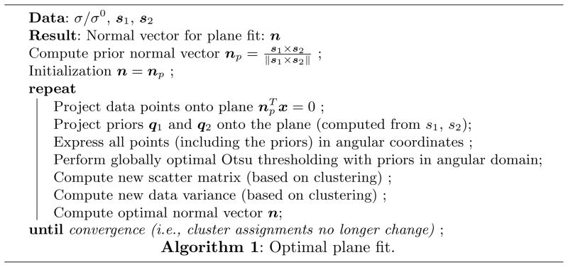
Once the plane has been fit, estimates of stain intensities are computed as the medians of the clusters. Estimates of the stain vectors are obtained by computing the robust minima (γ-percentile) and maxima ((1 − γ) percentile) within the cluster centers; γ = 1 for all experiments performed here. These estimates enable the transformation of images into any chosen color-space, and therefore normalization of appearance across multiple slides. While related to the approach by [3] the proposed method alleviates problems with uneven cluster sizes by defining statistics within the clusters, by weighting the plane fit with respect to cluster size, and by incorporating prior information. The benefits of this new approach are presented in Sec. 5. Fig. 1 shows an overview of the plane fitting algorithm with prior.

Fig. 1.

Algorithmic description of the optimal plane-fit algorithm.

5 Validation and Experimental Results

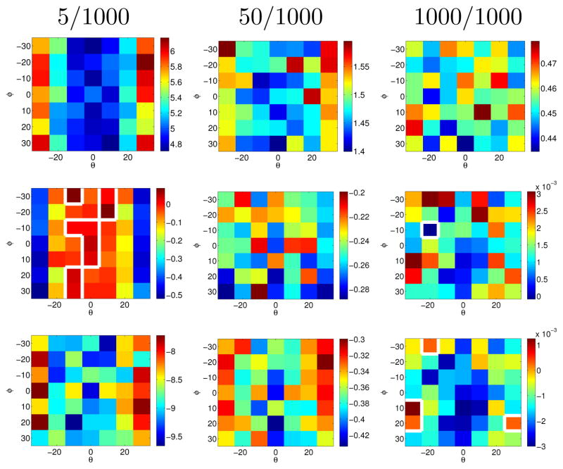
Figs. 3, 2 and 4 show the performance of the plane fitting algorithm with prior. Fig. 3 shows the results of a synthetic experiment to estimate the plane normal. Three methods are compared: (1) estimation without a plane normal prior (corresponding to the method in [3]), (2) estimation with a plane normal prior, but without the clustering step, and (3) the full algorithm 1. Estimation results shown are deviations (in degrees) of the estimated normal vector n̂ with respect to the ground truth normal vector. To assess the influence of varying cluster sizes and normal priors, two stain vectors s₁, s₂ were chosen at a 15 degree angle. Varying numbers of stain vectors were generated for the two stains using an isotropic Gaussian distribution (standard deviation of 0:1 which is similar to that in our real data sets). Priors were generated from the stain vectors by tilting the normal vector by an angle θ with respect to the axis defined by the stain vectors (translated to the origin) and by rotating the priors within the plane by an angle Φ. Fig. 3 shows that all three methods to determine the plane normal have similar performance for clusters of equal size. Prior information improves the results greatly for uneven point distributions (by almost 10 degrees on average for the most extreme point imbalance 5/1000 as expected to occur for example in regions with sparsely distributed nuclei). In cases where the effect of the prior is most pronounced, the clustering further improves estimation results.

Fig. 3.

Synthetic experiments: Angle difference (in degrees) between the estimated normal vector and the ground truth. Top row: proposed method. Middle row: plane fit with prior without clustering error minus with clustering error. Bottom row: plane fit without prior error minus plane fit with prior with clustering error. Estimates are results of 1000 random samples for different priors and varying numbers (5/1000, …) of points in the two stain clusters. The proposed method performs best. The white line shows the zero level set of angle differences.

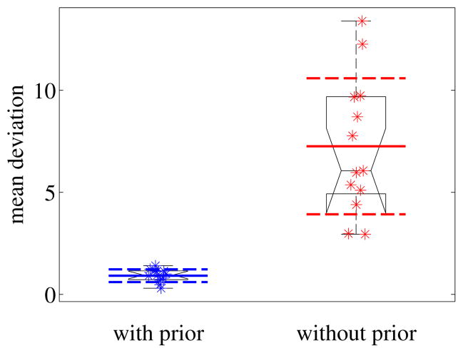
Fig. 2.

Estimation consistency for the proposed method and the method not using prior information [3] comparing the mean deviation from the mean normal vector across a slide (with respect to the tiles) in degrees. Smaller values and a tighter distribution demonstrate the advantage of the proposed method. Results are statistically significantly different.

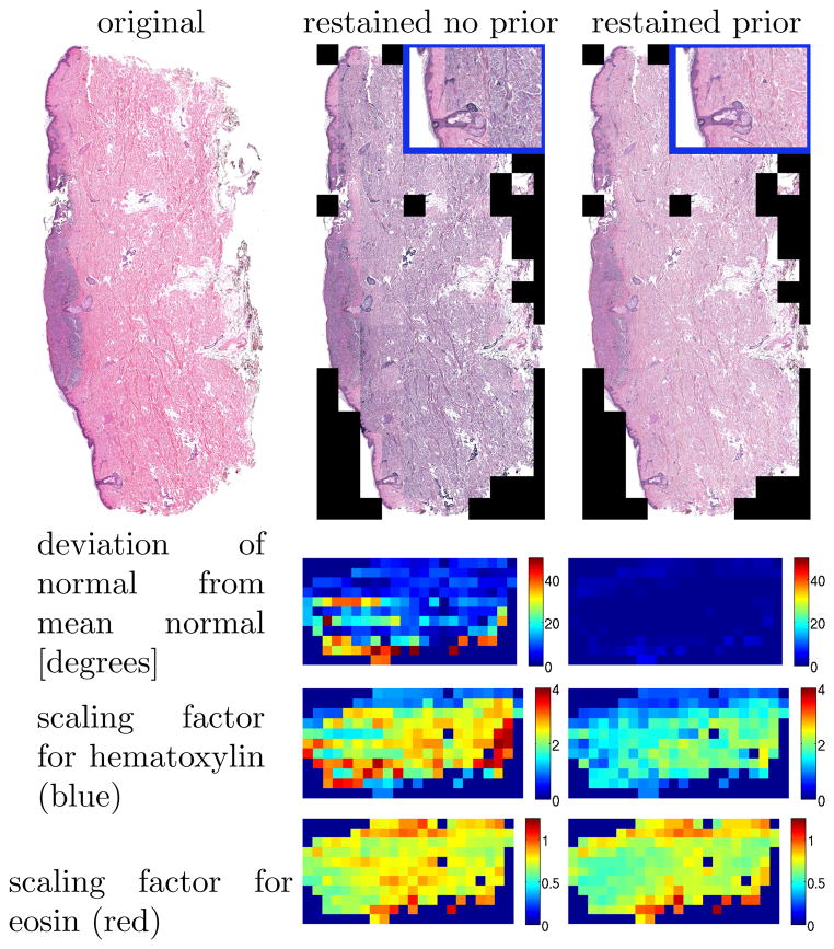
Fig. 4.

Restaining of a real dataset using the proposed method (right) and the method not using prior information (middle). Zoom-ins (top-right).

Fig. 2 shows the performance of the method on 13 real datasets compared to direct plane fitting without a plane prior as in [3]. The histology images were subdivided into areas of 1000×1000 pixels and were independently adjusted for stain intensity and stain direction using the two methods. Fig. 2 shows the estimation consistency for the two methods by comparing the mean deviation from the mean normal vector across a slide (mean with respect to the tiles). Estimation consistency is statistically significantly better for the proposed method (with p < 1e−4 using a t-test or non-parametric permutation test). The mean deviation from the prior was around 11 degrees for the method using prior information and 20 degrees for the method not using the prior information. The tight distribution for the consistency results for the proposed method demonstrates that the prior was not chosen to dominate the results.

To illustrate the behavior of the estimation method graphically Fig. 4 shows the results for a real dataset compared to direct plane fitting without a plane prior. Stain intensity scaling factors and the deviations from the mean of the estimates for the normal direction are shown. For a well working method, the results are expected to be approximately uniform. While the difference for the stain correction between the two methods (in both cases prior information was used for the clustering to obtain the intensity scalings) is not as drastic as for the normal direction, the plane fitting method with prior improves intensity scalings as can be witnessed by the reconstruction results, which are almost perfectly uniform for the method using prior information and inconsistent otherwise.

6 Conclusions

This paper presented a method to automatically adjust the appearance of stained histology slides. It described a novel way of adding prior information for the stain vectors and how to deal with unequal stain distribution through a clustering process. The clustering is a novel adaptation of Otsu thresholding including prior information. The underlying optimization problem relates to trust-region optimization and is therefore well studied and easy to solve. Real and synthetic experiments showcase the superior performance of the method developed.

References

- 1.Ruifrok A, Johnston D. Quantification of histochemical staining by color de convolution. Analytical and Quantitative Cytology and Histology. 2001 Aug;23:291–299. [PubMed] [Google Scholar]
- 2.Rabinovich A, Agarwal S, Laris C, Price J, Belongie S. Unsupervised color decomposition of histologically stained tissue samples. Advances in Neural Information Processing Systems. 2003 [Google Scholar]
- 3.Macenko M, Niethammer M, Marron J, Borland D, Woosley J, Guan X, Schmitt C, Thomas N. A method for normalizing histology slides for quantitative analysis. Proceedings of the Sixth IEEE International Symposium on Biomedical Imaging (ISBI) 2009:1107–1110. [Google Scholar]
- 4.Otsu N. A threshold selection method from gray-level histograms. Automatica. 1975;11:285–296. [Google Scholar]
- 5.Nocedal J, Wright SJ. Numerical Optimization. Springer; 2006. [Google Scholar]