

Abstract
Relatively few studies have characterized differences in intra- and inter-neighborhood traffic-related air pollutant (TRAP) concentrations and distance-decay gradients in along an urban highway for the purposes of exposure assessment. The goal of this work was to determine the extent to which intra- and inter-neighborhood differences in TRAP concentrations can be explained by traffic and meteorology in three pairs of neighborhoods along Interstate 93 (I-93) in the metropolitan Boston area (USA). We measured distance-decay gradients of seven TRAPs (PNC, pPAH, NO, NOX, BC, CO, PM2.5) in near-highway (<400 m) and background areas (>1 km) in Somerville, Dorchester/South Boston, Chinatown and Malden to determine whether (1) spatial patterns in concentrations and inter-pollutant correlations differ between neighborhoods, and (2) variation within and between neighborhoods can be explained by traffic and meteorology. The neighborhoods ranged in area from 0.5 to 2.3 km2. Mobile monitoring was performed over the course of one year in each pair of neighborhoods (one pair of neighborhoods per year in three successive years; 35-47 days of monitoring in each neighborhood). Pollutant levels generally increased with highway proximity, consistent with I-93 being a major source of TRAP; however, the slope and extent of the distance-decay gradients varied by neighborhood as well as by pollutant, season and time of day. Correlations among pollutants differed between neighborhoods (e.g., ρ = 0.35-0.80 between PNC and NOX and ρ = 0.11-0.60 between PNC and BC) and were generally lower in Dorchester/South Boston than in the other neighborhoods. We found that the generalizability of near-road gradients and near-highway/urban background contrasts was limited for near-highway neighborhoods in a metropolitan area with substantial local street traffic. Our findings illustrate the importance of measuring gradients of multiple pollutants under different ambient conditions in individual near-highway neighborhoods for health studies involving inter-neighborhood comparisons.
Keywords: near-highway, distance-decay gradients, mobile monitoring, traffic-related air pollution, metropolitan Boston (USA)
1. Introduction
Living near major roadways is associated with increased risks of cardiovascular and pulmonary disease (Gan et al., 2009; Hoek et al., 2013; McConnell et al., 2010). The possibility that exposure to traffic-related air pollution (TRAP) may play a role has motivated research to understand which, if any, of the many components of TRAP may be causative agents (Brugge et al., 2007; HEI, 2010).
Disentangling the effects of TRAP components in health studies requires an understanding of how pollutants are patterned in space and time, and the extent to which patterns differ by pollutant and across geographic settings. TRAP concentrations can vary significantly in both space and time near roadways (Karner et al., 2010; Levy et al., 2013). Sharp decreases in the concentration of many pollutants including elemental carbon (EC), black carbon (BC), carbon monoxide (CO), nitrogen oxides (NOX), particle number (PNC), and volatile organic compounds have been measured within 150 – 650 m of the edges of highways and major roads (Durant et al., 2010; Karner et al., 2010; Padró-Martínez et al., 2012; Pattinson et al., 2014; Roorda-Knape et al., 1998). The most-pronounced gradients occur for more reactive pollutants with low background concentrations, such as NO and ultrafine particles (UFP; <100 nm in diameter), and the least-pronounced gradients occur for relatively inert pollutants with elevated background concentrations (e.g., fine particle mass)(Zhou and Levy, 2007). In urban areas, spatial characterization can be complicated by street canyons and roadside structures such as noise barriers, elevated or depressed roadways, and buffers of trees and shrubs (Hagler et al., 2012; Hagler et al., 2010; Ning et al., 2010; Vardoulakis et al., 2003). Studies suggest that roadside structures tend to decrease near-road TRAP concentrations and increase on-road concentrations (Finn et al., 2010; Hagler et al., 2012; Ning et al., 2010; Steffens et al., 2014).
While previous efforts have focused on TRAP variation between cities (Eeftens et al., 2012; Fruin et al., 2014; Lebret et al., 2000) and within cities (Clougherty et al., 2008; Dons et al., 2013; Duvall et al., 2012; Jerrett et al., 2005; Levy et al., 2014), there are relatively few reports on the extent to which TRAP concentrations and spatial distributions measured in one near-highway neighborhood can be generalized to other neighborhoods along the same highway. Studies are needed that characterize TRAP variation at fine scales – e.g., <~5 km2 neighborhoods – for the purpose of developing accurate estimates of TRAP exposures in urban populations. Because spatial distributions of TRAP are also affected by factors that vary by season or time of day (such as wind patterns, temperature, and emissions source strength)(Kassomenos et al., 2014; Levy et al., 2013), measurement campaigns aimed at characterizing spatial differences in near-highway TRAP in neighborhoods should be performed over time. One way to measure differences in TRAP distance-decay gradients and temporal trends near highways is to conduct mobile monitoring along a highway in a single urban area in different seasons and times of day.
The goal of our study was to characterize gradients of seven TRAPs (PNC, pPAH, NO, NOX, BC, CO, PM2.5) in three near-highway (<400 m) and three background (>1000 m from nearest interstate highway) urban neighborhoods in the metropolitan Boston area (Massachusetts, United States). Our specific objectives were to determine whether (1) spatial patterns in concentrations and inter-pollutant correlations differ between neighborhoods, and (2) variation within and between neighborhoods can be explained by traffic and meteorology. We hypothesized that for each study area TRAP concentrations would be higher near highways than in urban background areas, and that pollutant distance-decay gradients could be explained in terms of traffic and meteorology. In particular, we expected that gradients would be similar in neighborhoods with single highways compared to neighborhoods with multiple major roadways and tall buildings, and that TRAP concentrations and the composition of TRAP mixtures would change in response to temporally-variable forcings. This work was performed as part of the Community Assessment of Freeway Exposure and Health study (CAFEH), a community-based participatory research (CBPR) study of TRAP exposure and cardiovascular health risk (Fuller et al., 2013).
2. Material and Methods
2.1. Study Area Descriptions
TRAP concentrations were measured in three demographically-matched pairs of near-highway (NH) and urban background (UB) neighborhoods in the Boston metropolitan area: Somerville (NH and UB), Dorchester/South Boston (NH and UB), Chinatown (NH) and Malden (UB; Figure 1). Study areas were relatively small, ranging in size from 0.5 km2 (Chinatown) to 2.3 km2 (Somerville; Table 1). Near-highway neighborhoods were defined as being 0-400 m from the nearest edge of Interstate 93 (I-93), which carries an average daily traffic (ADT) load of 1.5x10⁵ vehicles per day (vpd; Central Transportation Planning Staff, 2012). Diesel vehicles accounted for 3.8% of I-93 traffic and <5% of traffic on local roads (Callahan, 2012; McGahan et al., 2001).
FIGURE 1.

Mobile Monitoring Areas And Driving Routes. Somerville Near-Highway (A) And Urban Background (B) Were Monitored FRom September 2009 Through August 2010; Dorchester Near-Highway (C) And Urban Background (D) Were Monitored FRom September 2010 Through August 2011; Chinatown (Near-Highway; E) Malden (Urban Backgroung; F) Were Monitored From August 2011 Through July 2012. “Dep#0042” Is A Boston Epa Speciation Trends Network Site (Id: 25-025-0042). Road Layers FRom Massgis (2008A).
Table 1.
Study areas.
| Area | Area (km2) | Monitoring period | Interstate Highways | Other major roadsa | Local diesel sourcesb | Buildings and roadside structures | Topographic featuresc |
|---|---|---|---|---|---|---|---|
| Somerville | 2.3 | Sept. 2009 to Aug. 2010 | I-93 (elevated in parts as much as 6 m, curves SE of study area)d | MA-28 (50); Broadway (14) | trucks <500 vpd; 200 trains/day ~100 m NE of background area | residences (~10-m high); 400-m-long noise barrier east of I-93 (3-m high) | 17 m hill east of I-93; 41 m hill between near-highway and urban background areas |
| Dorchester | 1.5 | Sept. 2010 to July 2011 | I-93 (3-6 m below grade) | Dorchester Ave (20), Old Colony Rd (36), Columbia Rd (20), and Adams St (9) | <500 vpd; 110 trains/day adjacent to west side of I-93 | residences (~10 m high); noise barrier along west side of I-93 (5-m-high) | 34 m hill east of I-93; east to west elevation increase from 0 m to 30 m |
| Chinatown | 0.5 | Aug. 2011 to July 2012 | I-93 (at-grade),e I-90 (below grade) | All other roads on the TAPL route (2 or 9) | <500 – 1000 vpd; buses plus 347 trains/dayf | residences and commercial buildings (up to 100-m tall); street canyonsg | 2-8 m above sea level |
| Malden | 0.7 | Aug. 2011 to July 2012 | None | MA-60 (20) | <500 vpd; 58 trains/day | Residences (mostly ~10 m high, some 6-8 story apartments) | 7–18 m above sea level |
Other highways and major roads in the study areas with their average daily traffic 4 in thousands of vehicles per day from MassGIS (2008b).
Diesel truck volumes from Callahan (2012) and Central Transportation Planning Staff (2012). Estimated diesel train volumes are the total of commuter (http://www.mbta.com/uploadedfiles/documents/2014%20BLUEBOOK%2014th%20Edition.pdf) and AMTRAK (http://www.amtrak.com/train-schedules-timetables) trains near and in the study areas.
Elevation data was obtained from the Massachusetts Digital Elevation Model (MassGIS, 2005). Building heights and number of floors from http://skyscraperpage.com/cities/maps/?cityID=145.
The I-93 corridor in Somerville also includes Mystic Avenue, which contributes 30,000 vehicles per day (vpd) at grade (Central Transportation Planning Staff, 2012).
The I-93 central artery tunnel comes above ground just northeast of the study area, and I-93 is elevated along the study area.
A train and bus depot (South Station) is located east of I-93 near the study area and commuter rail (diesel) train tracks run along I-90 southeast of the study area.
The tallest two buildings in the Chinatown study area are 92 m (25 stories) and 79 m (23 stories).
Mobile monitoring in all three pairs of neighborhoods was conducted over the course of a year (Table 2; Figure S1). Monitoring was conducted in Somerville (Figures 1A and 1B) from September 2009 to August 2010. Somerville air pollution sources were dominated by major roadways, including I-93, state highways, and a collector road. Route-38 (Mystic Avenue, ADT = 30,000 vpd), a four-lane state highway adjacent to I-93 in Somerville, was defined as part of the I-93 highway corridor (Central Transportation Planning Staff, 2012). Monitoring was conducted in Dorchester and South Boston, herein referred to as “Dorchester” (Figures 1C and 1D), from September 2010 to July 2011. In this area, I-93 runs parallel to railroad lines about 3 m to 6 m below grade. Monitoring in Chinatown (Figure 1E) and Malden (Figure 1F) was performed between August 2011 and July 2012. Chinatown is located in downtown Boston and contains many major roadways and street canyons. The neighborhood is also near South Station, a regional transportation hub for trains and buses. Chinatown is flanked on its east side by I-93 and bisected east to west by I-90 (~90,000 vpd; Central Transportation Planning Staff, 2012). A residential neighborhood in Malden with similar demographics was selected as the background area to pair with Chinatown because all of Chinatown was <400 m from I-93. The Malden study area contains a diesel bus terminal and two commuter rail stations. More details on key features of each study area are available in Table 1 and Supporting Information (SI) Section 2.
Table 2.
Summary of monitoring years and site conditions during monitoring.
| Somerville | Dorchester | Chinatown | Malden | ||
|---|---|---|---|---|---|
| Year | 9/2009–8/2010 | 9/2010–8/2011 | 8/2011–7/2012 | 8/2011–7/2012 | |
| # of monitoring days | 44 | 35 | 47 | 36 | |
| # of monitoring hours | 281 | 173 | 141 | 85 | |
| # April – October hours a | 152 | 90 | 83 | 57 | |
| # November – March hours a | 129 | 83 | 58 | 28 | |
| Parameter | |||||
| Wind speed, m/sb | 2.6 (1.6) | 3.0 (2.1) | 2.9 (1.6) | 2.4 (1.3) | |
| Temperature, °Cb | 11.05 (16.6) | 9.15 (11.1) | 14.4 (10.6) | 14.8 (13.8) | |
| Day of week, percent of full dataset | Sun | 6% | 10% | 10% | 2% |
| Mon | 8% | 11% | 4% | 8% | |
| Tues | 18% | 10% | 19% | 11% | |
| Wed | 27% | 24% | 20% | 33% | |
| Thurs | 24% | 15% | 13% | 32% | |
| Fri | 4% | 17% | 21% | 9% | |
| Sat | 14% | 12% | 14% | 5% | |
| I-93 Traffic volume, vphb | 8500 (1800) | 9600 (1000) | 9600 (1400) | N/A | |
| I-93 Traffic speed, kphb | 83 (29) | 86 (15) | 86 (16) | N/A | |
| I-90 Traffic volume, vphb | N/A | N/A | 7086(3526) | N/A | |
| I-90 Traffic speed, kphb | N/A | N/A | 90 (5) | N/A | |
Monitoring hours are split into warm (April to October) and cold (November to March) months.
Data are summarized by mean with interquartile range in parentheses.
2.2. Data Collection
Mobile monitoring was conducted with the Tufts Mobile Air Pollution Monitoring Laboratory (TAPL), a gasoline-powered vehicle that was driven on fixed routes (not on I-93) in each neighborhood (Figure 1; details in SI 2 and Padró-Martínez et al., 2012). Each route took 40-60 minutes to complete and was driven in 2-6 hour shifts on each day of monitoring. Monitoring was conducted on 35-47 days (85-281 hours) in each neighborhood in the morning, afternoon, and evening in winter, spring, summer, and fall on non-consecutive days selected to maximize variability in meteorological and traffic conditions (Table 2, Table S1). In Somerville and Dorchester, the near-highway and urban background areas were close enough that they could be monitored on the same day; however, Chinatown (near-highway) and Malden (background) were too far apart to monitor both neighborhoods on the same day (11 km), so monitoring in these two neighborhoods was conducted up to 8 days apart (mean difference = 2 days). The TAPL measured PNC, NO, NOX, CO, BC, particle-bound polycyclic aromatic hydrocarbons (pPAH), and fine particulate mass (PM2.5; Table S2). Measurement averaging times ranged from 1-s (PNC) to 60-s (BC) and the distance between measurements was 5-600 m. Quality control measures included side-by-side instrument comparisons, flow checks, and lag-time corrections. To avoid inclusion of measurements tainted by self-sampling of exhaust from the TAPL, data were censored for TAPL speeds <5 km/h (~14% of data was censored). In Chinatown, correction of the GPS coordinates was sometimes necessary due to weak satellite signals in street canyons.
Meteorological, traffic, and geographical data were obtained from public datasets and assigned to each pollutant measurement using SAS 9.2 (see Figure 1 for site locations). Wind speed and direction (7.9 m above ground level) and temperature (2 m above ground level) data were measured at Logan International Airport (NCDC, 2012). This meteorological station was selected because of high data completeness across all three years of monitoring (~99%), and it provides a better estimate of regional meteorology than of local meteorology, especially in the case of Chinatown where there are many street canyons. Hourly highway traffic counts and speed were measured by the Massachusetts Department of Transportation using remote traffic microwave sensors (model X3; stakeholder.traffic.com). Distance to highway edge was obtained by conducting spatial joins of measurement locations with a highway polygon in ArcGIS (Lane et al., 2013).
2.3. Data Analysis
To determine whether monitoring in the three study areas in different years impacted our results, we compared hourly measurements of CO, NO, and NOX and daily measurements of PM2.5 collected continuously throughout the 3-year study period at the EPA Speciation Trends Network site (EPA-STN; ID: 25-025-0042) in Boston. This site is located ~1,500 m west of I-93 and in a mixed residential and commercial area (Figure 1; MA DEP, 2012). Interannual differences in CO, NO, NOX, and PM2.5 between September 2009 and July 2012 were tested using a multiple comparison Kruskal-Wallace test at the 95% confidence level (Giraudoux, 2013; Graves et al., 2012). To test for potential bias due to monitoring on different days in Chinatown and Malden, NO, NOX, and CO measurements collected at the EPA-STN site during the hours of monitoring in the two neighborhoods were compared using the Kruskal-Wallace tests at the 95% confidence interval. PM2.5 data were only available for every third day and were therefore not included in the analysis comparing monitoring days in Chinatown and Malden.
The one-sided Wilcoxon rank sum test (95% CI) was used to determine whether near-highway pollutant concentrations were statistically higher than concentrations in the paired urban background area. Spatial gradients in the near-highway areas were visualized with loess smoothing windows (spans) between 0.10 and 0.75. The spans with the least smoothing (smallest span) that had little noise were presented with 95% confidence intervals from generalized additive models (GAMs; Hastie, 2013). Smooths are presented instead of scatterplots because the large number of points (>160,000 per study area) interferes with scatterplot readability and interpretability.
The effects of temporal factors including meteorology and traffic volume on air pollutant concentrations were explored using several visualization tools. Loess smooths and boxplots were used to explore the impacts of individual factors like temperature and wind speed. Polar plots were used to explore the joint effects of wind speed and wind direction on pollutant concentrations (Carslaw and Ropkins, 2012).
Spearman correlations were calculated between hourly median pollutant concentrations in each near-highway and urban background area to reduce the impact of individual spikes. Spearman correlations were also generated for different times of the day as well as for different seasons. These correlations may change over short time periods due to differences between fresh and aged pollutants; therefore, the sensitivity of correlations to aggregation time was tested by comparing Spearman correlations for hourly medians with those for monthly, daily, and 1-minute medians for a subset of the data. The 1-min aggregation time matched the resolution of the BC monitor, which had the longest reporting interval of all the monitors. All statistical analyses were performed in R (R Core Team, 2013).
3. Results
3.1. Effects of Non-simultaneous Monitoring
Differences related to non-simultaneous monitoring as measured at the EPA-STN site in Boston were small or statistically insignificant; therefore, we did not adjust our measurements to reflect the non-simultaneous measurement periods. Interannual differences in median NO, NOX, CO, and PM2.5 concentrations measured at the EPA-STN site were low: <2 ppb, <2 ppb, <5 ppb, and <0.1 μg/m3, respectively (Figure 2). PM2.5 was statistically the same across all three years (Kruskal-Wallace multiple comparisons, p=0.89). There was also no statistical difference between NOX in the first two years or CO in the second two years (p>0.05 for all). Trends in concentrations of CO, NO, and NOX were not expected to affect the comparison among neighborhoods (all changed at a rate of <3 ppb/year; p<0.001), and there was no statistically significant trend in PM2.5 (p>0.99). In comparing NO, NOX, and CO concentrations at the EPA-STN site during the hours of non-simultaneous monitoring in Chinatown and Malden, there was no significant difference in NO or NOX (Kruskal-Wallace multiple comparisons, p = 0.23 and 0.87, respectively); however, CO concentrations were higher during monitoring in Malden (p=0.03; Figure S2). The median CO concentrations measured at the EPA-STN site were 232.6 ppb during the hours of monitoring in Chinatown and 265.0 ppb during the hours of monitoring in Malden. This difference suggests there may have been some bias in the CO results: as much as 25% of the difference between Malden and Chinatown CO (Table 3) can be attributed to monitoring on different days in the two neighborhoods.
FIGURE 2.
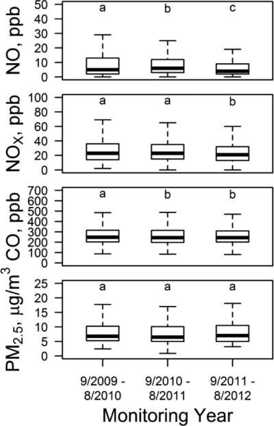
Tukey Boxplots Comparing No, Nox, Co, And PM2.5 Measure At Stn Site 25-025-0042 In Boston (Figure 1) For Each Full Mobile Monitoring Year. Whisker Lengths Are The Smaller Value Of 1.5*Iqr And The Distance To The Maximum Or Minimum (Outliers Not Shown). Common Letters Above The Boxes for Each Pollutant Identify Groups That Are Not Significantly Different At the 95% Condidence Interval Using Kruskal-Wallace Mulpiple Comparisons Test. Data is From Ma Dep (2012)
Table 3.
Summary of pollutant measurements for each study area.
| Somervillea | Dorchestera | Chinatown/Maldena | |||||||
|---|---|---|---|---|---|---|---|---|---|
| NH | UB | Pb | NH | UB | Pb | NH | UB | Pb | |
| CO, ppb | 390 (310) | 310 (230) | <0.001 | 600 (420) | 660 (450) | 1c | 460 (380) | 344 (280) | <0.001 |
| NO, ppb | 15 (26) | 6 (11) | <0.001 | 31 (50) | 32 (46) | 0.50 | 16 (24) | 8 (15) | <0.001 |
| NOx, ppb | 33 (39) | 20 (20) | <0.001 | 67 (56) | 71 (54) | 0.55 | 36 (35) | 20 (27) | <0.001 |
| pPAH, fA | 8 (12) | 4 (6) | <0.001 | 5 (8) | 3 (5) | <0.001 | 8 (11) | 3 (5) | <0.001 |
| PNC, 1000 cm−3 | 30 (49) | 18 (19) | <0.001 | 27 (33) | 19 (20) | <0.001 | 26 (26) | 14 (20) | <0.001 |
| PM2.5, μg m−3 | 15 (23) | 14 (17) | <0.001 | 13 (8) | 14 (7) | 1c | 14 (9) | 12 (9) | <0.001 |
| BC, μg m−3 | 0.8 (0.9) | 0.5 (0.5) | <0.001 | 0.4 (0.4) | 0.3 (0.3) | <0.001 | 0.8 (0.9) | 0.5 (0.5) | <0.001 |
Median pollutant levels with IQR in parentheses for NH = near-highway (<400m from edge of I-93) and UB = urban background (>1000 m from edge of I-93) areas.
P-values are based on Wilcoxon rank sum test of the null hypothesis that near-highway concentrations are ≤ urban background concentrations.
Urban background concentrations were statistically significantly greater than near-highway concentrations.
3.2. Spatial Differences
Near highway – urban background contrasts were not the same for all pollutants in all neighborhoods. In Somerville and Chinatown, concentrations of all seven pollutants were higher near I-93 compared to urban background; however, in Dorchester only PNC, pPAH, and BC were higher near I-93 compared to background (Wilcoxon rank sum test, p<0.001)(Table 3; Figure 3). In Dorchester the median concentrations of NOX and NO were not statistically different near I-93 compared to background, and median concentrations of CO and PM2.5 were actually higher in the background area than near the highway. The highest concentrations of gaseous pollutants in Dorchester tended to occur when winds were from the west (Figure S3). Empirical cumulative distributions in Figure 3 show that intra-neighborhood differences were greater than inter-neighborhood differences for PNC and pPAH, while for CO, NO, NOX, PM2.5, and BC inter-neighborhood differences were greater than intra-neighborhood differences. In addition, Dorchester had particularly high levels of NO, NOX, and CO and low levels of BC compared to the other neighborhoods.
FIGURE 3.

Empirical Cumullative Distribution Functions For Particles (Left Side: Pm2.5, Pnc, Ppah, BC) And Gases (Right Side: Co, No, NoX) For Someriville Near-Highway (Nh) And Urbam Backgrougn (Ub), Dorchester Near-Highway And Urban Background, Chinatown Near-Highway, And Malden Urban Background Study Areas. The X-Axis Maxima Were Set At The 99Th Percentile Of Near-Highway Measurements In Somerville.
Pollutant distance-decay gradients generally reached background within 200 m of I-93 when significant local sources were absent; therefore, 200 m was used as the cutoff for near-highway gradient calculations. Distance-decay gradients near I-93 were different for each near-highway neighborhood, with the steepest gradients occurring in Somerville and Dorchester (Figure 4). In Somerville and Dorchester PNC decreased by 34% and 30%, respectively, between 0-200 m from I-93, while the PNC distance-decay gradient in Chinatown was generally flat (2.2%; Table 4). Similarly, pPAH also decreased more in Dorchester (44%) and Somerville (39%) compared to Chinatown (21%). Somerville had the most pollutants with decreases of >20% within the first 200 m from I-93: PNC, BC, NO, NOX, and pPAH. In Dorchester, only PNC and pPAH decreased by >20%. In Chinatown, CO, NO, and pPAH decreased by ~21% and all other pollutants decreased by <20%. The gradients from I-93 were stronger than those from I-90 in Chinatown: BC decreased by 8% and PNC decreased by 1%, while CO, NO, and NOX increased by <8.3% over 200 m from I-90 and neither pPAH nor PM2.5 had a significant trend over the same distance (Figure S4). In all three neighborhoods, PNC and pPAH had statistically significant distance-decay gradients within 200 m of I-93. In some cases, increasing pollutant concentrations with distance from I-93 were observed at distances greater than 200 m. In addition to those pollutants already mentioned, PNC and pPAH increased from 200 to 400 m west of I-93 in Dorchester as distance to a major urban roadway (Dorchester Avenue) decreased.
FIGURE 4.

Loess Smooths (Black Lines) With 95% Confidence Intervals (Grey Shading) For Pnc, Pm2.5, Ppah, Bc, Co, No, And Nox, As A Function Of Distance From The Nearest Edge Of I-93 (Vertical Black Lines) For Somerville (Left), Dorchester (Center), And Chinatown/Malden (Right). Each Plot Has A Break Between The Near-Highway And Urban Background. The Only Urban Background Area East Of I-93 Is Malden. Distances East Of I-93 Are Positive And Distances West Of I-93 Are Negative.
Table 4.
Distance-decay gradients of pollutant concentration within 200 m of highway edge.
| Somerville: I-93 | Dorchester: I-93 | Chinatown: I-93 | Chinatown: I-90 | |||||||||
|---|---|---|---|---|---|---|---|---|---|---|---|---|
| Estimatea | Decrease, % | Estimatea | Decrease, % | pb | Estimatea | Decrease, % | pb | Estimatea | Decrease, % | pb | ||
| PNC | −0.204 | 33.5 | <0.001 | −0.176 | 29.7 | <0.001 | −0.011 | 2.2 | 0.003 | −0.005 | 1 | <0.001 |
| BC | −0.17 | 29 | 0.0007 | −0.03 | 6 | 0.4 | −0.02 | 4 | 0.7 | −0.04 | 8 | 0.001 |
| CO | −0.007 | 1 | 0.3 | 0.009 | −2 | 0.3 | −0.121 | 21.5 | <0.001 | 0.040 | −8.3 | <0.001 |
| NO | −0.21 | 34 | <0.001 | −0.01 | 2 | 0.6 | −0.12 | 21 | <0.001 | 0.021 | −4.3 | <0.001 |
| NOx | −0.130 | 23 | <0.001 | −0.01 | 2 | 0.4 | −0.07 | 10 | <0.001 | 0.012 | −2.4 | <0.001 |
| pPAH | −0.25 | 39 | <0.001 | −0.29 | 44 | <0.001 | −0.12 | 21 | <0.001 | 0.002 | −0.4 | 0.7 |
| PM2.5 | −0.02 | 4 | 0.09 | −0.016 | 3.1 | 0.08 | 0.029 | −6.0 | <0.001 | −0.001 | 0.2 | 0.8 |
Estimate is the % change in the logarithm of the pollutant concentrations per 100 m away from the edge of the highway. It was obtained by multiplying the coefficient of the simple log-linear regression of concentration as a function of distance times 100.
The percent decrease over 200 m is calculated as 100*[exp(Estimate/100*200)-1] (Wooldridge, 2012). Decreases ≥ 20% are bold.
P-value for the Estimate coefficient.
3.3. Temporal Differences
The effects of I-93 traffic volume were not the same for all pollutants in the three near-highway neighborhoods. PNC increased sharply in the three neighborhoods when traffic volumes were >~9,000 vehicles/hr (Figure S5), particularly during the morning rush hour when winds were lightest and (presumably) mixing height was lowest. Also, PM2.5 generally increased with traffic volume in the three neighborhoods, and pPAH, CO, NO, and NOx increased with traffic volume in Dorchester. In contrast, compared to differences among the neighborhoods, BC was largely unchanged with traffic volume, and pPAH, CO, NO, and NOx concentrations were relatively unchanged as traffic increased in Somerville and Chinatown.
The effects of temperature on pollutant concentrations were similar for all neighborhoods. Temperature is an independent factor affecting air pollution formation and removal rates as well as a proxy for other seasonal factors (e.g., photochemical activity, mixing height). Temperature most strongly affected PNC and PM2.5, which were highest in winter and summer, respectively (Figure S6). Other pollutants (CO, NO, NOX, pPAH, BC) had small or non-monotonic changes with temperature. Likewise, the effects of wind speed were similar for all neighborhoods: concentrations generally decreased with increasing wind speed (Figures S3 and S7). Exceptions were PM2.5 in Somerville and BC in Somerville and Dorchester, which increased in both magnitude and variability above ~6 m/s.
Effects of wind direction were different in each neighborhood. While the monitored near-highway areas generally had elevated pollutant concentrations when they were downwind of I-93, some areas also had high pollutant concentrations when the wind came from other directions (Figure S3). These differences were clearest for PNC, which had high concentrations for southeast winds in Somerville and Malden, northeast winds in Dorchester, and north and east winds in Chinatown. In Dorchester, concentrations of CO, NO, and NOX were 2-4 times higher than in other neighborhoods and exceeded mean hourly concentrations in the study area for westerly winds (i.e., as high as 900 ppb CO, 60 ppb NO, and 100 ppb NOX). In Chinatown, pollutant concentrations in the Washington Street canyon (which runs north-south) were highest for south winds from the direction of I-90 and lowest for north winds and west winds (Figure 5). Differences in concentrations for different wind directions were largest for PM2.5 and smallest for NO and NOX.
FIGURE 5.

Tukey Boxplots Of Co, No, No2 Nox, Ppah, Pnac, Pn2.5, Bc Concentrations On Washington Street (Street Canyon In Chinatown) As A Function Of Wing Direction Relative To The Street Orienatation. Whisker Lengths Are The Smaller Value Of 1.5*Iqr And The Distance To The Maximum Or Minimum (Outliers Not Shown).
3.4. Inter-pollutant Correlations
Inter-pollutant correlations varied by neighborhood. Spearman correlations were higher among the gases (NO, NOX, and CO) and lower among particulate pollutants (Figure 6). PNC was more highly correlated with the gases than with measures of particle mass. The correlations of NO with NOX were consistently high in both near-highway and urban background areas in Somerville, Dorchester, and Chinatown/Malden. In general, correlations were lower in Dorchester than in other areas; the only correlation greater than 0.7 in the Dorchester near-highway area was for NO and NOX (0.93). In contrast, the Somerville near-highway area had high correlations for many pollutant pairs, including NOX and CO (0.76), NOx and pPAH (0.83), and NOx and PNC (0.80). As expected, PM2.5 was not highly correlated with other pollutants in any of the study areas. Inter-pollutant correlations also varied by season and time of day: correlations were higher in cold months (November to March) than in warm months (April to October; Figure 7), and correlations were high during the morning rush hour (particularly when winds were light), low during the middle of the day, and high again during the afternoon rush hour (Figure 8).
FIGURE 6.

Spearman Correlations of Pollutions (Hourly Median) By Study Area.
FIGURE 7.

Spearman Correlations For Warm (April To October) And Cole (November To March) Months For Someville, Dorchester, Chinatown, And Malden. The Bc Monitor Was Not Running During The Cold Months In Somerville.
FIGURE 8.

Spearman Correlations In Each Study Area By Time Of Day. Morning = 04:30-10:00, Midday = 10:00-14:00, And Afternoon = 14:00-22:00.
A sensitivity analysis performed with the Chinatown data demonstrated that correlations were sensitive to aggregation times: correlations were usually higher for daily and hourly medians compared to 1 month and 1 min medians (Figure S8). Most inter-pollutant correlations were highest for measurements aggregated by day, although correlations of PM2.5 with BC, PNC, and pPAH and of pPAH with BC were highest for monthly aggregation.
4. Discussion
We compared spatial and temporal TRAP trends in three near-highway and three urban background neighborhoods in a single urban corridor. Although each neighborhood had similar levels of local and diesel traffic and mobile source pollution and low levels of industrial or power plant emissions (Callahan, 2012; MassGIS, 2008a; U.S. Energy Information Administration, 2014), there were different spatial patterns in TRAP concentrations and inter-pollutant correlations. Pollutant levels generally increased with highway proximity, consistent with I-93 as a major TRAP source; however, distance-decay gradients varied by neighborhood in addition to season and time of day. In general, our results are consistent with studies that have reported pronounced distance-decay gradients of TRAP <200 m from highways and higher concentrations of TRAP near highways than in urban background neighborhoods (Durant et al., 2010; Hu et al., 2012; Kassomenos et al., 2014; Kittelson et al., 2004; Zhu et al., 2009). Previous studies have reported differences in air pollution in different neighborhoods (e.g., Bereznicki et al., 2012; Duvall et al., 2012; Fruin et al., 2014; Kassomenos et al., 2014); however, these differences were generally attributed to local sources such as industrial plants, power generation, or marine shipping terminals. Unlike Fruin et al (2014), we found only small differences in PM2.5 (≤3 μg/m3) between neighborhoods, possibly because of the more substantial regional contribution to PM2.5 in the Boston area relative to Southern California, as well as because the neighborhoods we monitored were closer together on average (1-30 km) than those in California (4-100 km).
Neighborhood geography including highway elevation and curvature, near-highway structures, and surface roads may help to explain observed differences in spatial variation of TRAP in the study neighborhoods. In Somerville, the influence of the elevated section of I-93 was larger than that of I-93 in Dorchester and I-90 in Chinatown, where the highway influence was likely reduced because the highways were below-grade (Steffens et al., 2014). Highway sections with large curvature (e.g., I-93 southeast of Somerville) potentially contributed to increased peak concentrations due to larger effective traffic volumes. On the other hand, noise barriers may have decreased peak concentrations east of I-93 in Somerville and west of I-93 in Dorchester (Finn et al., 2010; Hagler et al., 2012; Ning et al., 2010). In Chinatown, street-canyons between tall buildings may have altered wind flow so that meteorological data from Logan Airport was not representative of wind direction and speed within the study area. The general results in Chinatown, particularly for winds from the south, were consistent with entrainment of highway-generated TRAP in a street canyon (Kumar et al., 2008). In addition, examination of concentration patterns indicated contributions from major surface roads were often comparable in magnitude to contributions from highways. This effect was largest in Dorchester and Chinatown, where at-grade traffic on major roads may have had more influence than direct emissions from I-93 and I-90. For example, Kneeland St and E Berkeley St contribute to air pollution in Chinatown because they provide access to highway ramps and have high-volume intersections (Massachusetts Bay Transportation Authority, 2005).
Although monitoring in all three near-highway areas was conducted over a similar range of meteorological and traffic conditions, some differences in pollutant concentrations and distance-decay gradients in the neighborhoods could not be explained by highway traffic data or data from the regional meteorological station. Traffic on local roadways may explain some of those differences, particularly in Dorchester, where CO and NOX concentrations were consistently higher than in other neighborhoods. Our study was not designed to formally capture sources other than highway vehicles, but evidence regarding different wind direction effects in the different neighborhoods can be used to generate hypotheses regarding important non-highway sources. For example, high PNC concentrations occurred for wind directions (including southeast in Somerville and Malden, northeast in Dorchester, and east in Chinatown) when the neighborhoods were downwind of downtown Boston and Logan Airport, which contain several potential emissions sources including surface transportation (roads and rail) and aircraft.
Correlations were generally strongest during times when there were high levels of fresh emissions (e.g., during rush hour) and during colder months (October-May). Higher correlations during cold months are consistent with the literature and may also be related to more favorable formation conditions for certain pollutants (e.g., ultrafine particles), greater atmospheric stability and lower photochemical activity during cooler times of the year (Kittelson et al., 2004; Kumar et al., 2014; Venkatram et al., 2013). These differences are unlikely to be related to traffic volume, which differed by ≤3% between warm and cold seasons. Correlations are useful to test our understanding of the sources and mixing; correlations among pollutants emitted from the same source should be high, while lower correlations may indicate another source or the presence of aged TRAP. Higher inter-neighborhood variation of PM2.5 than intra-neighborhood variation (one-way ANOVA) and generally low correlations of PM2.5 with the other pollutants suggest that PM2.5 was more regional while the other pollutants had local sources, consistent with expectations.
There were limitations in our data collection and analysis methods. First, the study was conducted with hourly meteorological data from a single weather station that was ~4-12 km from the study areas. Local wind effects such as wind tunnels between rows of buildings were not captured by the station at Logan Airport. Second, traffic parameters were based on highway counts. TRAP sources that are not captured in the available datasets (e.g., diurnal variation in congestion and diesel traffic on local roads) may also explain some of the observed inter-neighborhood differences. Third, distance-decay gradients measured by the mobile laboratory for pollutants with longer measurement times (BC, NO, NOX, CO) may be underestimated; therefore, comparison of distance-decay gradients would possibly have yielded different results had all the monitors recorded measurements at the same frequency. These limitations do not significantly affect our main result that there are both intra- and inter-neighborhood differences in TRAP along I-93 in the Boston area.
The finding that the near-highway neighborhoods are different in terms of TRAP has two main implications for health studies in small areas. First, distance-decay gradients measured in one near-highway neighborhood are not necessarily transferable to other neighborhoods, even along the same highway in a metropolitan area. In health studies involving comparison of different neighborhoods, monitoring in multiple locations at different times may be required to characterize gradients particularly where there are (1) pronounced changes in highway grade or curvature, or (2) changes in near-highway structures, vegetation, and building height or density. Second, consideration of multiple pollutants may be necessary given that the causal pollutant(s) within TRAP have not yet been delineated. Using a single surrogate pollutant may lead to differential error across neighborhoods, as the surrogate will represent different combinations of pollutants across locations. The variable patterns within a day suggest that these differences may be particularly important in short-term studies, which will need to account for multi-pollutant correlations that change in both space and time.
5. Conclusions
Our results indicate that generalizability of near-road gradients and near-highway/urban background contrasts is limited for near-highway neighborhoods in a metropolitan area with substantial mobile source emissions. Near-highway distance-decay gradients of TRAP concentrations and inter- pollutant correlations were not the same in different neighborhoods along a single highway through an urban area. Differences were not completely explained by temporal variation, including traffic patterns or seasonal or diurnal effects. These differences may be related to local infrastructure, traffic congestion, and non-traffic sources of air pollution. Our results suggest that caution should be used when assuming similarity of near-highway areas for epidemiological studies because even measuring several gradients at different locations along a highway may underestimate the true variability in distance-decay gradients in urban areas. These findings may be particularly relevant for metropolitan areas like Boston where, due to roadside structures, highway geometry, and local wind and traffic patterns, near-highway neighborhoods will exhibit dissimilar air pollution impacts from mobile sources.
Supplementary Material
Highlights.
We compared traffic-related air pollution in 3 Boston-area neighborhoods near I-93.
Pollutant distance-decay gradients were different in each neighborhood.
Pollutant correlations varied by neighborhood, season, and time of day.
Acknowledgments
This work was done as part of the Community Assessment of Freeway Exposure and Health (CAFEH) study, a CBPR project. The CBPR Community Partners were the Somerville Transportation Equity Partnership, the Committee for Boston Public Housing, the Chinatown Resident Association, and the Chinese Progressive Association. Jeffrey Trull, Kevin Stone, Piers MacNaughton, Eric Wilburn, Andrew Shapero, Samantha Weaver, Alex Bob, and Dana Harada contributed to the data collection and processing effort. Tina Wang and Baolian Kuang provided local knowledge on Chinatown and Kevin Stone provided local knowledge on Somerville. We would like to thank the members of the CAFEH Steering Committee: Ellin Reisner, Boalian Kuang, Lydia Lowe, Edna Carrasco, M. Barton Laws, Yuping Zeng, Michelle Liang, Christina Hemphill Fuller, Mae Fripp, Kevin Lane, and Mario Davila. We are also grateful to George Allen at NESCAUM for the generous loan of the aethalometer. This research was supported by NIEHS (ES015462) and the Jonathan M. Tisch College of Citizenship and Public Service (through the Tufts Community Research Center). APP was partially supported by the US EPA (FP-917203), NIEHS (T32 ES198543), and a P.E.O. Scholar award. This work has not been reviewed by any governmental agency. The views expressed are solely those of the authors, and governmental agencies do not endorse any products or commercial services mentioned in this paper.
Footnotes
Publisher's Disclaimer: This is a PDF file of an unedited manuscript that has been accepted for publication. As a service to our customers we are providing this early version of the manuscript. The manuscript will undergo copyediting, typesetting, and review of the resulting proof before it is published in its final citable form. Please note that during the production process errors may be discovered which could affect the content, and all legal disclaimers that apply to the journal pertain.
References
- Bereznicki SD, Sobus JR, Vette AF, Stiegel MA, Williams RW. Assessing spatial and temporal variability of VOCs and PM-components in outdoor air during the Detroit Exposure and Aerosol Research Study (DEARS). Atmospheric Environment. 2012;61:159–168. [Google Scholar]
- Brugge D, Durant JL, Rioux C. Near-highway pollutants in motor vehicle exhaust: a review of epidemiologic evidence of cardiac and pulmonary health risks. Environ Health. 2007;6:23. doi: 10.1186/1476-069X-6-23. Epub 2007/08/11. doi: 10.1186/1476-069x-6-23. PubMed PMID: 17688699; PubMed Central PMCID: PMCPMC1971259. [DOI] [PMC free article] [PubMed] [Google Scholar]
- Callahan M. Memorandum: Results of the Boston Region MPO's 2010 Freight Study – A Profile of Truck Impacts. Boston Region Metropolitan Planning Organization; 2012. [Google Scholar]
- Carslaw DC, Ropkins K. openair — An R package for air quality data analysis. Environmental Modelling & Software. 2012;27–28:52–61. [Google Scholar]
- Central Transportation Planning Staff Average Daily Traffic on Massachusetts Roads, CTPS Geoserver. 2012 http://www.ctps.org/geoserver/www/apps/adtApp/index.html.
- Clougherty JE, Wright RJ, Baxter LK, Levy JI. Land use regression modeling of intra-urban residential variability in multiple traffic-related air pollutants. Environ Health. 2008;7:17. doi: 10.1186/1476-069X-7-17. Epub 2008/05/20. doi: 10.1186/1476-069x-7-17. PubMed PMID: 18485201; PubMed Central PMCID: PMCPMC2397396. [DOI] [PMC free article] [PubMed] [Google Scholar]
- Dons E, Temmerman P, Van Poppel M, Bellemans T, Wets G, Int Panis L. Street characteristics and traffic factors determining road users' exposure to black carbon. Sci Total Environ. 2013;447:72–9. doi: 10.1016/j.scitotenv.2012.12.076. Epub 2013/02/05. doi: 10.1016/j.scitotenv.2012.12.076. PubMed PMID: 23376518. [DOI] [PubMed] [Google Scholar]
- Durant JL, Ash CA, Wood EC, Herndon SC, Jayne JT, Knighton WB, et al. Short-term variation in near-highway air pollutant gradients on a winter morning. Atmospheric chemistry and physics (Print) 2010;10(2):5599–626. doi: 10.5194/acpd-10-5599-2010. Epub 2010/01/01. PubMed PMID: 22427751; PubMed Central PMCID: PMCPMC3304588. [DOI] [PMC free article] [PubMed] [Google Scholar]
- Duvall RM, Norris GA, Burke JM, Olson DA, Vedantham R, Williams R. Determining spatial variability in PM2.5 source impacts across Detroit, MI. Atmospheric Environment. 2012;47:491–498. [Google Scholar]
- Eeftens M, Tsai M-Y, Ampe C, Anwander B, Beelen R, Bellander T, Cesaroni G, Cirach M, Cyrys J, de Hoogh K, De Nazelle A, de Vocht F, Declercq C, Dėdelė A, Eriksen K, Galassi C, Grąulevičienė R, Grivas G, Heinrich J, Hoffmann B, Iakovides M, Ineichen A, Katsouyanni K, Korek M, Krämer U, Kuhlbusch T, Lanki T, Madsen C, Meliefste K, Mölter A, Mosler G, Nieuwenhuijsen M, Oldenwening M, Pennanen A, Probst-Hensch N, Quass U, Raaschou-Nielsen O, Ranzi A, Stephanou E, Sugiri D, Udvardy O, Vaskövi É, Weinmayr G, Brunekreef B, Hoek G. Spatial variation of PM2.5, PM10, PM2.5 absorbance and PMcoarse concentrations between and within 20 European study areas and the relationship with NO2 – results of the ESCAPE project. Atmospheric Environment. 2012;62:303–317. [Google Scholar]
- Finn D, Clawson KL, Carter RG, Rich JD, Eckman RM, Perry SG, Isakov V, Heist DK. Tracer studies to characterize the effects of roadside noise barriers on near-road pollutant dispersion under varying atmospheric stability conditions. Atmospheric Environment. 2010;44:204–214. [Google Scholar]
- Fruin S, Urman R, Lurmann F, McConnell R, Gauderman J, Rappaport E, Franklin M, Gilliland FD, Shafer M, Gorski P, Avol E. Spatial variation in particulate matter components over a large urban area. Atmospheric Environment. 2014;83:211–219. doi: 10.1016/j.atmosenv.2013.10.063. [DOI] [PMC free article] [PubMed] [Google Scholar]
- Fuller CH, Patton AP, Lane K, Laws MB, Marden A, Carrasco E, Spengler J, Mwamburi M, Zamore W, Durant John L, Brugge D. A community participatory study of cardiovascular health and exposure to near-highway air pollution: study design and methods. Reviews on Environmental Health. 2013;28:21. doi: 10.1515/reveh-2012-0029. [DOI] [PMC free article] [PubMed] [Google Scholar]
- Gan WQ, Tamburic L, Davies HW, Demers PA, Koehoorn M, Brauer M. Changes in residential proximity to road traffic and the risk of death from coronary heart disease. Epidemiology. 2010;21(5):642–9. doi: 10.1097/EDE.0b013e3181e89f19. Epub 2010/06/30. doi: 10.1097/EDE.0b013e3181e89f19. PubMed PMID: 20585255. [DOI] [PubMed] [Google Scholar]
- Giraudoux P. pgirmess: Data analysis in ecology. 2013 http://CRAN.R-project.org/package=pgirmess.
- Graves S, Piepho H, Selzer L, Dorai-Raj S. multcompView: Visualizations of Paired Comparisons. 2012 http://CRAN.R-project.org/package=multcompView.
- Hagler GSW, Lin M-Y, Khlystov A, Baldauf RW, Isakov V, Faircloth J, Jackson LE. Field investigation of roadside vegetative and structural barrier impact on near-road ultrafine particle concentrations under a variety of wind conditions. Science of The Total Environment. 2012;419:7–15. doi: 10.1016/j.scitotenv.2011.12.002. [DOI] [PubMed] [Google Scholar]
- Hagler GS, Thoma ED, Baldauf RW. High-resolution mobile monitoring of carbon monoxide and ultrafine particle concentrations in a near-road environment. J Air Waste Manag Assoc. 2010;60(3):328–36. doi: 10.3155/1047-3289.60.3.328. Epub 2010/04/20. PubMed PMID: 20397562. [DOI] [PubMed] [Google Scholar]
- Hastie T. gam: Generalized Additive Models, R package version 1.08. 2013 http://CRAN.R-project.org/package=gam.
- HEI Traffic-Related Air Pollution: A Critical Review of the Literature on Emissions, Exposure, and Health Effects. HEI Panel on the Health Effects of Traffic-Related Air Pollution. 2010 [Google Scholar]
- Hoek G, Krishnan R, Beelen R, Peters A, Ostro B, Brunekreef B, Kaufman J. Long-term air pollution exposure and cardio-respiratory mortality: a review. Environmental Health. 2013;12:43. doi: 10.1186/1476-069X-12-43. [DOI] [PMC free article] [PubMed] [Google Scholar]
- Hu S, Paulson SE, Fruin S, Kozawa K, Mara S, Winer AM. Observation of elevated air pollutant concentrations in a residential neighborhood of Los Angeles California using a mobile platform. Atmospheric Environment. 2012;51:311–319. doi: 10.1016/j.atmosenv.2011.12.055. [DOI] [PMC free article] [PubMed] [Google Scholar]
- Jerrett M, Arain A, Kanaroglou P, Beckerman B, Potoglou D, Sahsuvaroglu T, Morrison J, Giovis C. A review and evaluation of intraurban air pollution exposure models. Journal of Exposure Analysis and Environmental Epidemiology. 2005;15:185–204. doi: 10.1038/sj.jea.7500388. [DOI] [PubMed] [Google Scholar]
- Karner AA, Eisinger DS, Niemeier DA. Near-roadway air quality: synthesizing the findings from real-world data. Environ Sci Technol. 2010;44(14):5334–44. doi: 10.1021/es100008x. Epub 2010/06/22. doi: 10.1021/es100008x. PubMed PMID: 20560612. [DOI] [PubMed] [Google Scholar]
- Kassomenos PA, Vardoulakis S, Chaloulakou A, Paschalidou AK, Grivas G, Borge R, Lumbreras J. Study of PM10 and PM2.5 levels in three European cities: Analysis of intra and inter urban variations. Atmospheric Environment. 2014;87:153–163. [Google Scholar]
- Kittelson DB, Watts WF, Johnson JP. Nanoparticle emissions on Minnesota highways. Atmospheric Environment. 2004;38:9–19. [Google Scholar]
- Kumar P, Fennell P, Britter R. Effect of wind direction and speed on the dispersion of nucleation and accumulation mode particles in an urban street canyon. Science of The Total Environment. 2008;402:82–94. doi: 10.1016/j.scitotenv.2008.04.032. [DOI] [PubMed] [Google Scholar]
- Kumar P, Morawska L, Birmili W, Paasonen P, Hu M, Kulmala M, Harrison RM, Norford L, Britter R. Ultrafine particles in cities. Environment International. 2014;66:1–10. doi: 10.1016/j.envint.2014.01.013. [DOI] [PubMed] [Google Scholar]
- Lane KJ, Kangsen Scammell M, Levy JI, Fuller CH, Parambi R, Zamore W, et al. Positional error and time-activity patterns in near-highway proximity studies: an exposure misclassification analysis. Environ Health. 2013;12(1):75. doi: 10.1186/1476-069X-12-75. Epub 2013/09/10. doi: 10.1186/1476-069x-12-75. PubMed PMID: 24010639; PubMed Central PMCID: PMCPMC3907019. [DOI] [PMC free article] [PubMed] [Google Scholar]
- Lebret E, Briggs D, van Reeuwijk H, Fischer P, Smallbone K, Harssema H, Kriz B, Gorynski P, Elliott P. Small area variations in ambient NO2 concentrations in four European areas. Atmospheric Environment. 2000;34:177–185. [Google Scholar]
- Levy I, Mihele C, Lu G, Narayan J, Brook JR. Evaluating Multipollutant Exposure and Urban Air Quality: Pollutant Interrelationships, Neighborhood Variability, and Nitrogen Dioxide as a Proxy Pollutant. Environmental Health Perspectives. 2013;122:65–72. doi: 10.1289/ehp.1306518. [DOI] [PMC free article] [PubMed] [Google Scholar]
- Levy I, Mihele C, Lu G, Narayan J, Hilker N, Brook J. Elucidating multipollutant exposure across a complex metropolitan area by systematic deployment of a mobile laboratory. Atmospheric Chemistry and Physics. 2014;14:7173–7193. [Google Scholar]
- MA DEP . Air Quality Monitoring Data from Site 25-025-0042. Massachusetts Department of Environmental Protection; 2012. [Google Scholar]
- Massachusetts Bay Transportation Authority Silver Line Phase III: Supplemental Draft EIS/EIR, Boston, MA. 2005 http://www.mbta.com/uploadedfiles/About_the_T/T_Projects/T_Projects_List/CH%204%20Final%20DEIS.pdf.
- MassGIS EOTMAJROADS, Office of Geographic and Environmental Information (MassGIS). Commonwealth of Massachusetts Executive Office of Energy and Environmental Affairs. 2008a [Google Scholar]
- MassGIS EOTROADS, Office of Geographic and Environmental Information (MassGIS). Commonwealth of Massachusetts Executive Office of Energy and Environmental Affairs. 2008b [Google Scholar]
- McConnell R, Islam T, Shankardass K, Jerrett M, Lurmann F, Gilliland F, Gauderman J, Avol E, Kunzli N, Yao L, Peters J, Berhane K. Childhood incident asthma and traffic-related air pollution at home and school. Environ Health Perspect. 2010;118:1021–1026. doi: 10.1289/ehp.0901232. [DOI] [PMC free article] [PubMed] [Google Scholar]
- McGahan A, Quackenbush KH, Kuttner WS. Regional Truck Study. Boston Region Metropolitan Planning Organization, Central Transportation Planning Staff. 2001 [Google Scholar]
- NCDC Integrated Surface Hourly (ISH) dataset, Logan International Airport, AWSMSC 725090, WBAN 14739. National Climate Data Center. 2012 ftp://ftp.ncdc.noaa.gov/pub/data/
- Ning Z, Hudda N, Daher N, Kam W, Herner J, Kozawa K, Mara S, Sioutas C. Impact of roadside noise barriers on particle size distributions and pollutants concentrations near freeways. Atmospheric Environment. 2010;44:3118–3127. [Google Scholar]
- Padro-Martinez LT, Patton AP, Trull JB, Zamore W, Brugge D, Durant JL. Mobile monitoring of particle number concentration and other traffic-related air pollutants in a near-highway neighborhood over the course of a year. Atmospheric environment (Oxford, England : 1994) 2012;61:253–64. doi: 10.1016/j.atmosenv.2012.06.088. Epub 2012/11/13. doi: 10.1016/j.atmosenv.2012.06.088. PubMed PMID: 23144586; PubMed Central PMCID: PMCPMC3491988. [DOI] [PMC free article] [PubMed] [Google Scholar]
- Pattinson W, Longley I, Kingham S. Using mobile monitoring to visualise diurnal variation of traffic pollutants across two near-highway neighbourhoods. Atmospheric Environment. 2014;94:782–792. [Google Scholar]
- R Core Team R: A language and environment for statistical computing, 2.13.1 ed. R Foundation for Statistical Computing, Vienna, Austria. 2013 http://www.R-project.org/
- Roorda-Knape MC, Janssen NAH, De Hartog JJ, Van Vliet PHN, Harssema H, Brunekreef B. Air pollution from traffic in city districts near major motorways. Atmospheric Environment. 1998;32:1921–1930. [Google Scholar]
- Steffens JT, Heist DK, Perry SG, Isakov V, Baldauf RW, Zhang KM. Effects of roadway configurations on near-road air quality and the implications on roadway designs. Atmospheric Environment. 2014;94:74–85. [Google Scholar]
- U.S. Energy Information Administration Massachusetts State Profile and Energy Estimates. 2014 http://www.eia.gov/state/?sid=MA.
- Vardoulakis S, Fisher BE, Pericleous K, Gonzalez-Flesca N. Modelling air quality in street canyons: a review. Atmospheric Environment. 2003;37:155–182. [Google Scholar]
- Venkatram A, Snyder M, Isakov V. Modeling the impact of roadway emissions in light wind, stable and transition conditions. Transportation Research Part D: Transport and Environment. 2013;24:110–119. [Google Scholar]
- Wooldridge JM. Introductory econometrics: a modern approach. Cengage Learning. 2012 [Google Scholar]
- Zhou Y, Levy J. Factors influencing the spatial extent of mobile source air pollution impacts: a meta-analysis. BMC Public Health. 2007;7:89. doi: 10.1186/1471-2458-7-89. [DOI] [PMC free article] [PubMed] [Google Scholar]
- Zhu Y, Pudota J, Collins D, Allen D, Clements A, DenBleyker A, Fraser M, Jia Y, McDonald-Buller E, Michel E. Air pollutant concentrations near three Texas roadways, Part I: Ultrafine particles. Atmospheric Environment. 2009;43:4513–4522. [Google Scholar]
Associated Data
This section collects any data citations, data availability statements, or supplementary materials included in this article.