

Abstract
Objective
Develop an improved method for auditing hospital cost and quality tailored to a specific hospital’s patient population.
Data Sources/Setting
Medicare claims in general, gynecologic and urologic surgery, and orthopedics from Illinois, New York, and Texas between 2004 and 2006.
Study Design
A template of 300 representative patients from a single index hospital was constructed and used to match 300 patients at 43 hospitals that had a minimum of 500 patients over a 3-year study period.
Data Collection/Extraction Methods
From each of 43 hospitals we chose 300 patients most resembling the template using multivariate matching.
Principal Findings
We found close matches on procedures and patient characteristics, far more balanced than would be expected in a randomized trial. There were little to no differences between the index hospital’s template and the 43 hospitals on most patient characteristics yet large and significant differences in mortality, failure-to-rescue, and cost.
Conclusion
Matching can produce fair, directly standardized audits. From the perspective of the index hospital, “hospital-specific” template matching provides the fairness of direct standardization with the specific institutional relevance of indirect standardization. Using this approach, hospitals will be better able to examine their performance, and better determine why they are achieving the results they observe.
Keywords: Quality of care, outcomes research, health care research, cost
By far, the most common method to compare hospital outcomes is indirect standardization, often accomplished by dividing the observed number of patient events at a hospital by the expected number of patient events derived from the population (Fleiss, Levin, and Paik 2003; Iezzoni 2012) to get the traditional “O/E” metric. In some cases the observed number of events (O) is replaced by a predicted number of events (P), where P is a function of O, as is done for Medicare’s Hospital Compare random effects model, where the quantity “P/E” is reported (Krumholz et al. 2006a,b; Silber et al. 2010). At times, investigators prefer to report (O-E)/N rather than O/E, which has the advantage that the metric is clearly defined and stable even when E is near zero (Chassin et al. 1989; Silber, Rosenbaum, and Ross 1995). All approaches have one aspect in common, that being the reliance on each individual hospital’s own patient case mix to be used when comparing across hospitals.
The fact that the indirect standardization approach allows two hospitals with very different distributions of patients to be compared represents both a strength and weakness of the technique. In a sense, indirect standardization tries to describe what has happened when the hospital sees the mix of patients it usually sees, while direct standardization tries to describe what would happen if the hospital saw a mix of patients based on another population of interest. Direct standardization will utilize this external reference population to weight the results of the index hospital (Fleiss, Levin, and Paik 2003). Speaking informally, a hospital administrator trying to improve the care of the current patient population is interested in indirect standardization (i.e., would other hospitals do better with my patients?), while a patient looking at a ranking of hospitals to select one would be interested in direct standardization—(i.e., where would it be best for me to go if I resembled the typical patients used for direct standardization, or how well has the hospital done with other patients who have the condition for which I am being admitted).
On the one hand, judging a hospital based on its own patient population makes intuitive sense—the hospital is being judged on cases relevant to what it sees. While it may be convenient to compare hospitals even if they treat very different types of patients, a concern of indirect standardization is that two hospitals that see very different types of patients may be unfairly compared, as the lack of overlap in patient populations places a great deal of burden on the indirectly standardized model to appropriately account for these nonoverlapping patient factors. If the model fails to incorporate the important differences between each hospital’s patient populations, then the inferences concerning hospital comparison with O/E methods may be misleading.
An alternative approach that we have introduced is to use a form of direct standardization (Silber et al. 2014, this issue), that uses a template of patients and compares a multivariate matched set of patients across hospitals, thereby achieving closely overlapping patient distributions for observable variables—far more close on measured characteristics than if patients had been randomly assigned to hospitals. In this previous work we described how multivariate template matching, as a method to compare hospitals using direct standardization, produced excellent matches across 217 hospitals performing general and orthopedic surgery across three states. It had the strength that each hospital was evaluated with the same template; therefore, there was less concern about nonoverlapping patients, when hospitals did have overlapping patients to compare.
When a hospital’s Chief Medical Officer desires to know precisely how well his or her hospital performs on its own distribution of patients, and not on an external template that may not be representative of the type of patients seen at his or her specific hospital, then direct standardization may not be the method of choice. In other words, the Chief Medical Officer may want to know, “How well do we do with the patients we see?” In this article, we develop a new method to perform indirect standardization with multivariate template matching, and we introduce what we define as “hospital-specific template matching” a form of direct standardization with a hospital’s own patients (thereby resembling aspects of indirect standardization). This approach will allow a close look at how well a hospital performs on the patients it sees by constructing a template of patients representative of the hospital’s own patient distributions, finding other hospitals that also see similar patients to compare outcomes between the hospital of interest and other hospitals that can be matched to the index hospital’s template. In so doing, we hope to provide a new method to better implement indirect standardization analyses for improving a hospital’s quality of care specifically tailored to the index hospital’s most relevant patients—the patients they see.
Methods
Conceptual Model: The Hospital-Specific Template Match
The hospital-specific template audit answers the question: “How did our hospital perform for the patients we see compared to how our patients would have fared at other hospitals that see patients like them?” It is easiest to understand this template audit as analogous to a classroom examination, where the exam is only given to students who took the same courses. A fair exam asks each student the same or similar questions. A fair audit contrasts hospital performance on similar patients, that is, patients undergoing similar procedures with the same or similar comorbid conditions. There is one specific difference from the classroom exam analogy—for hospital-specific template matching, we construct an exam tailored to an individual student’s background. We then only compare that student’s grade to other students who took the same classes and were given the exam tailored to that first student. The hospital-specific template approach uses matching to enable a hospital to find peer hospitals that see patients like their own.
The template for hospital-specific template matching consists of a collection of 300 patients undergoing procedures performed at the hospital in question. It is constructed by taking a sample of 300 patients from the hospital of interest. In our case, the template will be a stratified random sample made up of 150 general surgery cases (with other procedures performed by general surgeons) and 150 orthopedic surgery cases.
To construct control hospital matched sets, 300 patients at each control hospital are identified that match the template for the index hospital of interest. The individual hospital’s constructed template (of size 300) is then individually paired to 300 patients at each of the other hospitals. If the first patient in the template is a 68-year-old woman with a prior heart attack undergoing hip surgery, then a similar patient is found at each of the other hospitals. This process of “matching” hospital patients to the template’s patients is accomplished using multivariate matching (Rosenbaum 2010b). Hospitals that do not have patients that can match the template are discarded from the comparison as described below. In the end, we will evaluate the index hospital by comparing its typical patients to a sequence of matched comparisons of similar patients at other hospitals. The index hospital sees outcomes and costs for 300 of its own patients together with summaries of outcomes for 300 similar patients at other hospitals. How would my patients fare elsewhere? Because these are 300 real patients at the hospital, not theoretical coefficients in a model, the Chief Medical Officer may examine its own patients with poor outcomes or excessive costs in as much detail as desired. Later, in Table 2, we present one such audit for one hospital, comparing its performance with 300 patients to the performance of 43 other hospitals with 300 very similar patients.
Table 2.
Auditing Hospital A’s Outcomes. We present a profile of Hospital A to illustrate the audit results. For each outcome we examine how Hospital A performed versus the 43 other hospitals on sets of matched patients that were very similar to those seen at Hospital A. We then examined for each outcome the orthopedic surgery and general surgery patients in the 43 hospitals not including Hospital A, to study how Hospital A fared in these patients undergoing different types of surgery. Letters denote p-values for comparing Hospital A to the 43 other hospitals. Percentile ranks (1 = best, 100 = worst)
| All Patients | Orthopedic Surgery Patients | General Surgery Patients | |||||||
|---|---|---|---|---|---|---|---|---|---|
| Outcomes (Percent Unless Otherwise Noted) | Hospital A N = 300 | 43 Other Hospitals N = 12,900 | Hospital A N = 150 | 43 Other Hospitals N = 6,450 | Hospital A N = 150 | 43 Other Hospitals N = 6,450 | |||
| % or Mean | Percentile | % or Mean | Percentile | % or Mean | Percentile | ||||
| Mortality | |||||||||
| Inpatient | 4.0***,†††† | 97 | 1.5 | 1.3 | 74 | 0.8 | 6.7****,†††† | 97 | 2.2 |
| 30-day | 5.3***,†††† | 97 | 2.3 | 2.0 | 66 | 1.8 | 8.7****,†††† | 97 | 2.9 |
| Complications | |||||||||
| Inpatient | 44.3 | 74 | 41.6 | 40.0 | 52 | 41.9 | 48.7* | 91 | 41.2 |
| 30-day | 51.7 | 33 | 55.4 | 48.0**,†† | 21 | 58.9 | 55.3 | 72 | 51.8 |
| FTR | |||||||||
| Inpatient | 9.0***,††† | 97 | 3.7 | 3.3 | 76 | 2.0 | 13.7***,†††† | 97 | 5.4 |
| 30-day | 10.3***,†††† | 97 | 4.4 | 4.2 | 80 | 3.0 | 15.7****,†††† | 97 | 5.8 |
| Readmissions | |||||||||
| 30-day | 10.3 | 77 | 8.9 | 10.0 | 74 | 8.2 | 10.7 | 70 | 9.6 |
| Total cost ($k) | |||||||||
| Inpatient | 11.7 | 52 | 11.7 | 10.2***,†† | 17 | 11.1 | 15.8**,††† | 93 | 13.0 |
| 30-day | 13.0 | 73 | 12.6 | 10.9**,† | 26 | 11.7 | 17.3**,††† | 93 | 14.1 |
| Total payment ($k) | |||||||||
| Inpatient | 13.4****,†††† | 28 | 15.2 | 13.7****,†††† | 20 | 15.8 | 12.2**,† | 42 | 13.1 |
| 30-day | 13.9****,†††† | 31 | 15.8 | 14.0****,†††† | 20 | 16.2 | 13.5**,† | 44 | 14.2 |
| Length of stay | |||||||||
| Overall | 4.5 | 31 | 4.7 | 4.1 | 40 | 4.4 | 5.1 | 52 | 5.1 |
| % of patients sent to ICU | 27.0****,†††† | 88 | 15.3 | 10.7 | 72 | 8.5 | 43.3****,†††† | 95 | 22.1 |
| Days in ICU, if sent to ICU‡ | 7.3† | 90 | 6.0 | 3.3 | 34 | 4.9 | 8.3†† | 95 | 6.5 |
| Procedure time (minutes) | 150.0****,†††† | 71 | 141.4 | 142.5 | 68 | 140.7 | 165.8****,†††† | 88 | 144.6 |
| Balance of Matched Variables | |||||||||
|---|---|---|---|---|---|---|---|---|---|
| Age (mean, years) | 76.3 | 76.0 | 77.2 | 76.8 | 75.5 | 75.2 | |||
| Gender (% male) | 42.7 | 42.2 | 37.3 | 36.7 | 48.0 | 47.6 | |||
| Procedure time (predicted) | 138.6 | 138.2 | 137.3 | 137.5 | 139.9 | 138.9 | |||
| Probability of 30-day death | 0.025 | 0.026 | 0.017 | 0.020 | 0.033 | 0.033 | |||
| Emergency admission | 16.0 | 16.5 | 16.7 | 17.3 | 15.3 | 15.8 | |||
| Transfer-in | 5.7 | 5.1 | 4.0 | 3.7 | 7.3 | 6.4 | |||
| Hx CHF | 17.0 | 16.7 | 14.7 | 14.3 | 19.3 | 19.1 | |||
| Hx arrhythmia | 23.0 | 22.8 | 18.7 | 18.5 | 27.3 | 27.0 | |||
| Hx MI | 11.3 | 10.4 | 11.3 | 10.2 | 11.3 | 10.6 | |||
| Hx angina | 4.0 | 3.8 | 2.7 | 2.7 | 5.3 | 4.9 | |||
| Hx diabetes | 27.0 | 26.4 | 22.7 | 22.2 | 31.3 | 30.6 | |||
| Hx renal dysfunction | 6.0 | 6.3 | 2.7 | 3.5 | 9.3 | 9.1 | |||
| Hx COPD | 17.3 | 17.4 | 12.0 | 12.5 | 22.7 | 22.4 | |||
| Hx of asthma | 14.3 | 13.4 | 12.7 | 11.6 | 16.0 | 15.1 | |||
Note. Mantel–Haenszel (binary variables) or stratified Wilcoxon rank-sum (continuous variables) p-value key: *p < .05; **p < .01; ***p < .001; ****p < .0001.
Conditional logit (binary variables) or m-estimation (continuous variables) p-value key: †p < .05; ††p < .01; †††p < .001; ††††p < .0001.
Conditional logit and m-estimation p-values account for paired differences in probability of death, predicted procedure time, transfer-in status, and emergency status. Length of stay means were calculated using trimmed means, excluding 2.5% of patients from each extreme. Total costs and payments are reported using Hodges–Lehmann estimates.
Tests for differences in days in ICU, if sent to ICU, are not paired due to the nature of the variable.
Constructing the Examination
For this research we examined the cost and quality of hospitals treating Medicare patients admitted for orthopedic and general surgery (including some urological and gynecological procedures often performed by general surgeons) throughout Illinois, New York, and Texas using the ICD-9-CM principal procedure codes found in the claims. We chose these states because their Medicare patients had a relatively low rate of managed care as compared to other states, and the states were geographically diverse. For these states we obtained the Medicare Part A, Part B and Outpatient files for the years 2004–2006, and merged these file to the Medicare Denominator File to determine dates of death and other demographic information.
We chose a template size of 300 because of practical size constraints and power considerations, though templates of various sizes can be constructed, depending on the purpose of the audit. Choosing a template of 300 prompted us to select hospitals that performed at least 500 cases over the 3 years of the dataset to ensure adequate matching ratios to achieve good matches at each hospital. Our study data set had 227 usable control hospitals, of which 43 hospitals did have a set of patients that matched Hospital A’s template.
Using a template with size 300 patients, we will wish to compare an outcome rate at a single hospital to the remaining 43 hospitals. In our study the factor under study is the hospital, or, in the experimental design literature, the hospital represents the “treatment of interest” and the patient is the “unit of analysis.” We ask whether the hospital/treatment produces poor outcomes in the patients who receive that treatment. Each patient in the index hospital is paired to 43 controls at other hospitals. To provide a rough sense of the statistical power for such a template size, we utilize the method of Miettinen (1969). For example, using a two-tailed type-I error of 5 percent, a hospital with an 8 percent death rate compared to a 4 percent rate for the remaining hospitals could be detected with above 90 percent power, and it would have 81 percent power for a hospital with a 7 percent mortality rate; and comparing a hospital with a 50 percent complication rate to the remaining hospitals with a 40 percent rate would obtain a power above 90 percent. We provide these power calculations only as a rough guide for the reader. The excellent power stems in part from the fact that each of 300 patients at one hospital is compared to 43 similar patients at 43 other hospitals, producing a comparison group of size 43 × 300 = 12,900 patients.
Administering the Examination
The process of giving the exam (performing the audit) involves the selection of 300 patients at each hospital who closely resemble the 300 patients in the template. We call this process “template matching” because at each hospital we choose 300 patients at that hospital that most reflect the 300 patients in the template: every hospital takes the same exam. To match 300 patients to the template requires some pool of patients at each hospital. As our template includes 150 general, gynecologic, and urologic surgery patients and 150 orthopedic patients, we only analyzed hospitals that saw at least 200 general, gynecologic, or urologic surgery patients and 300 orthopedic surgery patients.
The matching was accomplished using Medicare claims from 2004 to 2006 (approximately 3 years of data, less 3 months to allow for a look-back period when defining comorbidities). We performed our matches using R MIPMatch (Zubizarreta 2012; R Development Core Team 2013; Zubizarreta, Cerda, and Rosenbaum 2013) and specified the following algorithm for selecting matches to the overall template: Match exactly on principal procedure whenever possible; if not possible, match within a procedure cluster (a clinical group of procedures that resemble the index procedure; e.g., right versus left hemicolectomy; see Appendix); if not possible, then do not use this hospital as a control. Inside each hierarchical category, we choose a match based on the minimized medical distance between patients, where medical distance is defined through the Mahalanobis distance, similar to what was described above for choosing the template. Details concerning the elements of the Mahalanobis distance are provided in the Appendix.
To improve the quality of the matches between the template and the specific hospital, we utilized fine balance (Rosenbaum, Ross, and Silber 2007; Silber et al. 2007b, 2012; Rosenbaum 2010a; Yang et al. 2012) within general surgical and orthopedic patients. Fine balance says that if one must tolerate a mismatch on, say, CHF for one patient, then this mismatch must be counterbalanced by a mismatch for CHF in the opposite direction, so the number of patients with CHF at the hospital equals the number in the template. Fine balance ensured that if the template had, say 35 percent CHF cases for its 150 general surgical cases and 25 percent CHF for its orthopedic cases, each hospital also provided a 35 percent rate of CHF for its general surgical and 25 percent rate for its orthopedic surgery cases whenever possible, without absolutely requiring exact matches on CHF for each and every patient in the hospital with respect to the template, though the algorithm also preferred to do that as often as possible via minimizing the Mahalanobis distance function.
Grading the Fairness of the Examination
Ideally, for a fair exam, every hospital would have been tested on exactly the same 300 patients as every other hospital. Of course, this is not possible—yet we can evaluate the fairness of the examination or audit by observing how similar the characteristics of the matched patients are across hospitals. If each hospital’s 300 patients display similar patient characteristics, then we will define this as a fair exam. For each hospital we can formally test whether the matched patients at their hospital are similar to the template. We tested whether the hospital’s matched set was similar to the template using the “cross-match” test (Rosenbaum 2005; Heller, Rosenbaum, and Small 2010b; Heller et al. 2010a). The cross-match test determines whether a hospital could be distinguished from the template based on the patients in the hospital’s matched set. The cross-match test takes 600 patients, 300 from the template and 300 from the hospital, pairing patients with similar characteristics ignoring their origin in the template or the hospital. Does pairing similar patients tend to separate the hospital and the template? A cross-match occurs when someone in the template is matched to someone in the hospital, and many cross-matches suggest that patient characteristics do not distinguish hospital and template patients. Transformation of the number of cross-matches provides a distribution-free P-value testing the equality of the distributions and also an estimate of a population quantity, Upsilon, that measures the degree of overlap. A hospital whose matched patients were not significantly different from the template would display an insignificant P-value and an estimated Upsilon that is about ½ or greater than ½. Hospitals were also required to have no significant difference in the number of transfer-in patients based on Fisher’s Exact Test.
Grading the Hospital
Matching is done first, to create a fair exam, without viewing outcomes. Once the hospital matches have been deemed fair, through examining the quality of the matches and using the cross-match test, the matching process stops, and examination of patient outcomes, costs, or processes at the hospital can begin. This two-step process prevents multiple analyses to find an analysis that makes outcomes look good—it prevents editing the exam after the student has answered the questions (Rubin 2007, 2008).
Here, we examine in-hospital and 30-day mortality; in-hospital and 30-day complications; in-hospital and 30-day failure-to-rescue (Silber et al. 1992, 2007a); readmissions within 30 days of discharge; resource utilization-based costs and payments, both in-hospital and 30-day (Silber et al. 2012, 2013); length of stay; the percent of patients that were in the ICU and the length of ICU stay for those in the ICU; and a potential process metric available in the data set, operative procedure length as defined through the anesthesia bill (Silber et al. 2007c,d, 2011, 2013). Summary estimates of Medicare costs and payments for Hospital A and matched patients are reported using a Hodges–Lehmann estimate (Hollander and Wolfe 1999), which is the location estimate derived from and compatible with the Wilcoxon signed-rank statistic. Readmission is all-cause readmission for this example, and complications are defined as in previous work (Silber et al. 2007a, 2012) comprising 38 common complications that occur post-operatively. Each hospital audit would include a comparison of the outcomes at that hospital to the other 43 hospitals in the study. The audit will also include post match adjustments (Cochran and Rubin 1973; Rubin 1979; Silber et al. 2005) that are expected to be generally similar to the “stratified” rates since we have already performed extensive matching to produce similar patients at each hospital. The stratified analysis will be performed using a Mantel–Haenszel test for discrete variables (clustering on the template patient) and a stratified Wilcoxon rank sum test (Lehmann 2006). The adjustment model for each discrete outcome used conditional logistic regression clustering on the template matched patient adjusting for probability of death score, predicted procedure time, and an indicator for emergency admission. For each continuous outcome we used robust regression (Huber 1981; Hampel et al. 1986), adjusting for the same variables and an indicator variable describing the template patient to whom the observed patient was matched (Rubin 1979).
Results
Hospital and Patient Populations
We required that hospitals had at least 200 general surgery cases and 300 orthopedic cases over the 3-year period for us to include them in the analysis. Of 514 acute care facilities within Illinois, New York, and Texas that participate in Medicare’s Surgical Care Improvement Project, 241 met this size requirement. Of the 240 hospitals that serve as control hospitals for Hospital A, we had complete billing data on 227, and of these 227 we could successfully match 79 hospitals to Hospital A’s template. Of the 79 hospitals that were successfully matched to Hospital A’s template, 20 failed the cross-match test (p ≤ .05) despite being of adequate size and having full billing data. The matched samples for 16 of the remaining 59 hospitals had significantly fewer transfer-in patients than in Hospital A’s template (p ≤ .05) and therefore were excluded, as it would not be fair to compare Hospital A to hospitals with fewer of these high-risk patients.
Examining the Quality of the Matches
In Table 1, we examine how similar the hospital’s matched samples were across hospitals, and formally test the overall variation of patient characteristics and outcomes across hospitals using the Kruskal–Wallis test, a nonparametric version of the one-way ANOVA test (Kruskal and Wallis 1952) for each continuous variable of interest and the Pearson Chi-square test for each binary variable. The test is simply a benchmark, comparing the similarity of hospitals in our template match to the similarity of hospitals if patients had been randomly assigned to hospitals. The chi-square statistic for the Kruskal–Wallis test divided by its degrees of freedom is also reported. In a completely randomized clinical trial—that is, random assignment of patients to hospitals—the Kruskal–Wallis chi-square divided by degrees of freedom would have expectation = 1, and it would tend to be larger than 1 if patients differed more than expected by random assignment, and it would have expectation less than 1 if patients differ across hospitals less than expected under random assignment. Arguably, the exam looks fair if this chi-square ratio is less than 1.
Table 1.
Assessing if Patient Covariates and Outcomes Vary Significantly across Hospitals. We compare the variation among hospitals in patient covariates and outcomes to the variation that would have been expected had patients been randomly assigned to hospitals. After matching, the patients are more similar on measured covariates than expected by random assignment, yet very different on outcomes. For the χ2 statistics, a χ2/degrees of freedom (=42 for 43 hospitals) that is greater than 1 suggests more variation than random, and less than 1 suggests less variation than random. For financial outcomes and procedure time, we display the Hodges–Lehmann estimates, and we report the statistic and p-value using the Kruskal–Wallis test. Note that patient variables are very stable across hospitals, whereas hospital outcomes are not
| Percentile Range (Hospital Means or Hodges–Lehmann Estimates) | |||||||
|---|---|---|---|---|---|---|---|
| Patient Covariates | Lower Eighth (12.5th) | Lower Quartile (25th) | Median | Upper Quartile (75th) | Upper Eighth (87.5th) | Chi-Square Statistic/DF | p-value |
| Age (years) | 75.7 | 75.7 | 75.9 | 76.1 | 76.4 | 0.84311 | .7538 |
| Gender (% male) | 41.7 | 42.0 | 42.0 | 42.7 | 42.7 | 0.03734 | 1.0000 |
| Probability of 30-day death | 0.0238 | 0.0244 | 0.0260 | 0.0281 | 0.0290 | 0.27678 | 1.0000 |
| Predicted procedure time (minutes) | 137.5 | 137.7 | 138.2 | 138.7 | 138.9 | 0.39881 | .9998 |
| Emergency admission | 15.7 | 16.0 | 16.7 | 17.0 | 17.0 | 0.11402 | 1.0000 |
| Transfer-in | 3.3 | 4.3 | 5.7 | 5.7 | 5.7 | 0.67780 | .9451 |
| Comorbidities | |||||||
| CHF | 15.7 | 16.3 | 16.7 | 17.0 | 17.3 | 0.14154 | 1.0000 |
| Past arrhythmia | 22.0 | 22.3 | 22.7 | 23.0 | 23.7 | 0.11405 | 1.0000 |
| Past myocardial infarction | 10.0 | 10.3 | 10.7 | 10.7 | 10.7 | 0.09536 | 1.0000 |
| Angina | 3.3 | 3.3 | 3.7 | 4.0 | 5.0 | 0.49806 | .9977 |
| Diabetes | 26.0 | 26.3 | 26.3 | 26.7 | 27.0 | 0.03394 | 1.0000 |
| Renal dysfunction | 6.0 | 6.0 | 6.3 | 6.7 | 6.7 | 0.09357 | 1.0000 |
| COPD | 16.3 | 17.0 | 17.3 | 18.0 | 18.3 | 0.17837 | 1.0000 |
| Asthma | 13.0 | 13.0 | 13.3 | 13.7 | 13.7 | 0.10066 | 1.0000 |
| Percentile Range (Hospital Means or Hodges–Lehmann Estimates) | |||||||
|---|---|---|---|---|---|---|---|
| Outcomes | Lower Eighth (12.5th) | Lower Quartile (25th) | Median | Upper Quartile (75th) | Upper Eighth (87.5th) | Chi-Square Statistic/DF | p-value |
| Mortality (%) | |||||||
| Inpatient | 0.7 | 1.0 | 1.3 | 2.0 | 2.3 | 0.8914 | .6712 |
| 30-day | 1.3 | 1.7 | 2.3 | 3.0 | 3.3 | 1.2808 | .1049 |
| Complications (%) | |||||||
| Inpatient | 35.3 | 37.7 | 41.0 | 44.3 | 47.7 | 4.2587 | <.0001 |
| 30-day | 45.7 | 50.3 | 56.0 | 59.7 | 61.7 | 5.8927 | <.0001 |
| Failure-to-rescue (%) | |||||||
| Inpatient | 1.6 | 2.3 | 3.8 | 5.0 | 5.7 | 1.0430 | .3948 |
| 30-day | 2.2 | 2.9 | 4.0 | 5.7 | 6.6 | 1.7040 | .0030 |
| Readmissions | |||||||
| 30-day % | 6.7 | 7.7 | 8.7 | 10.0 | 10.7 | 1.6971 | .0032 |
| Length of stay* | 4.3 | 4.4 | 4.6 | 5.0 | 5.2 | 4.5715 | <.0001 |
| Patients in ICU (%) | 9.0 | 9.7 | 14.3 | 19.0 | 23.0 | 10.6930 | <.0001 |
| Days in ICU, if sent to ICU | 4.7 | 5.0 | 6.2 | 6.7 | 7.1 | 2.0811 | <.0001 |
| Total cost ($1,000s; Hodges–Lehmann estimates) | |||||||
| In-hospital $ | 10.7 | 11.1 | 11.7 | 12.1 | 12.4 | 5.5274 | <.0001 |
| 30-day $ | 11.5 | 11.9 | 12.5 | 13.0 | 13.5 | 4.7859 | <.0001 |
| Total payment ($1,000s; Hodges–Lehmann estimates) | |||||||
| In-hospital $ | 13.0 | 13.4 | 14.2 | 16.2 | 20.0 | 55.6498 | <.0001 |
| 30-day $ | 13.8 | 13.9 | 14.7 | 17.1 | 20.8 | 49.6518 | <.0001 |
| Procedure time (minutes) | 117.8 | 126 | 135.8 | 152.3 | 173.3 | 39.7043 | <.0001 |
Note. *Length of Stay means were calculated using trimmed means, excluding 2.5% of patients from each extreme.
We see that patient covariates across hospitals are very similar, far more similar than if the patients were randomly assigned to hospitals, as the chi-square ratios are generally far below 1. For major patient characteristics and hospital outcomes, Table 1 presents the hospital values for half the entire distribution (the median), then divided by quarters and then half again (12.5th and 87.5th percentiles). As can be seen, values of patient characteristics were very stable across hospitals, and this was supported by the chi-square ratios generally far below 1, and p-values near 1.000. (An expanded version of this table with all 20 matched comorbidities can be found in the Appendix.) The matching made groups of patients at different hospitals who look far more similar in terms of the variables in Table 1 than would have been expected by randomly assigning patients to hospitals. It is possible, of course, that patients differ in ways not recorded in Table 1.
Results from Table 1 suggest that the template matching produced sets of patients across hospitals that were very similar to each other, thereby allowing for fair comparison of hospital outcomes. The procedure matching algorithm was very successful: of 12,900 patients from the 43 matched hospitals, 12,161, or 94.3 percent, were exactly matched to their respective Hospital A template patient on ICD-9-CM principal procedure. The remaining patients were matched to template patients exactly on procedure cluster.
The bottom portion of Table 1 looks at outcomes, asking if similar patients at different hospitals have similar outcomes. Unlike patient characteristics, hospital outcomes varied greatly, and significantly, across institutions. Outcome rates differ among hospitals by far more than would be expected if hospitals provided equivalent care and patients were randomly assigned to hospitals. On covariates, patients look more similar than by random assignment, but on outcomes they look quite different. This is also described in Figure 1, where we examine each of the reported outcomes across the 43 hospitals with probability density plots, where the area under each distribution sums to a probability of 1.0.
Figure 1.
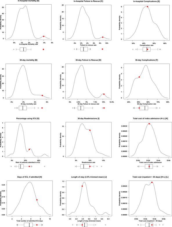
Hospital Outcomes. We display the outcomes for 43 hospitals, each hospital having 300 template-matched patients. For each outcome we provide density plots with an associated box plot providing 5th, 25th, 50th, 75th, and 95th percentile markers, as well as a depiction of outliers. We also denote individual Hospital A (examined in Table 2) as a large solid red dot on the plots. Displayed are (A) in-hospital mortality; (B) 30-day mortality; (C) in-hospital failure-to-rescue rate; (D) 30-day failure-to-rescue rate; (E) in-hospital complication rate; (F) 30-day complication rate; (G) percentage of patients using the ICU; (H) ICU LOS in patients using the ICU; (I) 30-day readmission rate; (J) Length of stay (2.5 percent trimmed mean); (K) total costs of the index admission (Hodges–Lehmann estimates); (L) total cost of the index admission, plus total costs 30 days after discharge from the index admission (Hodges–Lehmann estimates)
Examining the Individual Hospitals—The Hospital-Specific Hospital Audit
We can now proceed to audit an individual hospital—the main goal of this report. We examine Hospital A on the outcome and process metrics of interest, and we compare Hospital A to the rest of the 43 hospitals in the data set, since all hospitals were matched to the same initial template from Hospital A. For comparison purposes, Hospital A is the same hospital depicted as Hospital A in our companion manuscript on direct standardization using template matching (Silber et al. 2014, this issue).
In Figure 1 Hospital A is denoted with a large solid dot in all graphs. In Table 2 we observe that Hospital A displayed a higher in-hospital death rate (4.0 percent) than the grouped rate of the other 43 control hospitals (1.5 percent), or a rank ordering of 97th percentile, and a similar poor performance in 30-day mortality with a 5.3 percent death rate versus controls of 2.3 percent, and a 97th percentile score. Without any post-match adjustment, the death rates for in-hospital and 30-day mortality did reach statistical significance (p = .0002 in-hospital; p < .0001 30-day). With post-match adjustment for the probability of death, emergency room admission, transfer-in status, and predicted procedure time, both in-hospital and 30-day mortality retained high statistical significance (p < .0001 for both). Hospital A’s death rates appeared elevated for both orthopedic and general surgery, both displaying poor rank percentiles, but rates for general surgery were especially problematic—about triple the death rate of the 43 matched hospitals.
Compared to other hospitals, Hospital A displayed a lower 30-day orthopedic complication rate (48.0 percent vs. 58.9 percent, unadjusted p = .0049; adjusted p = .0065), but a nonsignificant and higher rate for general surgery (55.3 percent vs. 51.8 percent), so the 30-day complication rates were not consistent. Performance on failure-to-rescue (FTR) was generally poor and did reach statistical significance for both inpatient and 30-day FTR for both stratified and regression adjusted stratified results (both p < .001). Hospital A ranked poorly for FTR (97th percentile) for both inpatient and 30-day metrics, overall and within general surgery.
Readmission rate was unremarkable, as was overall length of stay. However, costs suggested an interesting pattern. One may look at overall costs and consider Hospital A to be an ordinary hospital. However, when looking within surgical groups, a different picture emerges. General surgical patient costs were very high compared to controls, whereas orthopedic surgery costs were quite low, so that these significant results cancelled themselves out to produce a neutral picture on cost overall.
The percentage of patients sent to the ICU was far higher than the remaining 43 hospital control rate (p < .0001), and the ICU stay per patient in the ICU was longer (p < .05 in the adjusted analysis). Finally, the Hodges–Lehmann estimate for surgical procedure time was over 8 minutes longer (p < .0001) at this hospital than the controls, despite the fact that predicted surgical times between cases and controls were almost identical (138.6 vs. 138.2 minutes).
When we examined the patient characteristics between this hospital and the remaining 43 hospitals at the bottom of Table 2, the rates were remarkably similar. It would appear that this hospital’s Chief Medical Officer would have difficulty building a case for defending their worse outcomes by suggesting that their patients were somehow sicker than the other 43 hospitals.
Finally, a sensitivity analysis (Rosenbaum 1988, 2002; Rosenbaum and Silber 2009) to explain away the higher mortality in Hospital A showed that an unobserved patient characteristic would need to triple the odds of being treated at Hospital A and triple the odds of death by 30 days.
Discussion
The hospital-specific template matching approach for auditing Hospital A represents a new approach to compare and understand hospital quality of care. We custom-made a template specifically for Hospital A to represent its unique patient mix. We then searched for other hospitals that did see these same patients. Our intent was to let Hospital A determine whether the patients it treats would have been better off going to another hospital. Though these other hospitals may see a different distribution of patients, these other hospitals did see enough similar patients to match Hospital A’s template so that the direct comparisons were feasible and fair. That is, by matching we found those 43 hospitals in our data set that had close enough overlap to be able to confidently use them as a control.
Similar to our previous results using direct standardization with template matching (Silber et al. 2014, this issue), the results of our analysis of general surgery and orthopedics displayed considerable differences in outcomes between Hospital A and the other 43 hospitals, despite very uniform patient characteristics across all hospitals. The hospital-specific template matching sample allows for a fair, directly standardized comparison across hospitals, since the matched sample of 300 patients is closely balanced between each hospital and the template. The resulting variation in outcomes between Hospital A and the 43 other hospitals was therefore believable and completely relevant to Hospital A because the template was based on Hospital A.
Hospital-specific template matching includes two desirable features of standardization methodology. There is a feature of direct standardization because all 43 hospitals and Hospital A were compared using the same template, which happens to be Hospital A’s template. It has as an important strength the similarity in patients that we observed in direct standardization using template matching (Silber et al. 2014, this issue). This similarity comes at some cost, in that we have fewer other hospitals that can be matched to Hospital A’s template. Using the method of direct standardization with template matching, we previously had found 217 hospitals that met the matching requirement, but this was accomplished with a template specifically made to be relevant to a larger group of hospitals. Another advantage of hospital-specific template matching is that the method includes some of the advantages of indirect-standardization. Hospital A can observe how well other hospitals would treat Hospital A’s patients because the template is constructed from Hospital A’s patients. This “boutique” match provides a unique perspective for Hospital A, since it would be harder to suggest that poor performance by Hospital A on the match constructed for Hospital A is simply due to different patient mix.
Selecting a peer group of hospitals that see patients like the index hospital’s patients may also aid in the construction of peer groups for assessing hospital quality. Methods to construct peer groups have traditionally utilized specific hospital characteristics (e.g., teaching vs. nonteaching), but they can also include a weighted mixture of characteristics. In fact, newer work has utilized a “nearest neighbor” approach to such selection of peers that minimizes a distance that includes whatever choice variables are desired (see Byrne et al. 2009). Utilizing our template approach in the peer selection algorithm may yet be another application for this work. A peer group based on hospitals that see similar patients may be more relevant than one based on a hospital characteristic such as teaching status.
Hospital-specific template matching may serve as a complement to template matching using direct standardization. We can envision insurers and policy makers screening and comparing hospitals on various templates they choose to construct, each relevant to specific policy initiatives and types of patients. Hospitals flagged as doing poorly can, on the other hand, ask whether other hospitals could have done better with their mix of patients. It should be stressed, however, that performing well on hospital-specific template matching does not negate the concerns raised on the direct standardization analysis. It simply suggests that the aspects of quality needed to do well on the direct template are lacking at this specific hospital, but luckily this hospital does not see many of those patients that need the strengths required for the direct template. Such distinctions are crucial to understand, especially for policy makers interested in optimal referral decisions and for individual hospital quality initiatives.
From the perspective of a hospital’s Chief Medical Officer, hospital-specific template matching combines the fairness of comparison from direct standardization with the specific institutional relevance of indirect standardization. With hospital-specific template matching, we believe CMOs will be better able to compare how their hospitals are performing with their own patient distribution, and better determine why they are achieving the results they observe.
Acknowledgments
Joint Acknowledgment/Disclosure Statement: We thank Traci Frank, A. A., and Alexander Hill, B. S., for their assistance on this project. This research was funded by grant R01-HS018338 from the Agency for Healthcare Research and Quality and grant NSF SBS-10038744 from the National Science Foundation.
Disclosures: None.
Disclaimers: None.
Supporting Information
Additional supporting information may be found in the online version of this article:
Appendix SA1: Author Matrix.
Table S1: Expanded Version of Table 1 (Assessing if Patient Covariates and Outcomes Vary Significantly across Hospitals).
Table S2: Expanded Version of Table 2 (Understanding an Individual Hospital’s Outcomes).
Table S3: Description of the Template Sample.
Table S4: Definitions of Index Surgical Populations and Hospitals.
Table S5: Description of Matching Algorithm.
Table S6: Description of Predicted Procedure Time Algorithm (A) Models Created to Predict Procedure Time; (B) Estimates, in Minutes, for All ICD-9-CM Principal Procedure-Secondary Procedure Interactions.
Table S7: Description of Procedure Group-Specific Models to Predict 30-Day Mortality.
Table S8: Definitions of ICD-9-CM Procedure Groups and Clusters.
Table S9: Definitions and Groupings of ICD-9-CM Secondary Procedures.
Table S10: Sensitivity Analysis.
References
- Byrne MM, Daw CN, Nelson HA, Urech TH, Pietz K. Petersen LA. Method to Develop Health Care Peer Groups for Quality and Financial Comparisons across Hospitals. Health Services Research. 2009;44(2 Pt 1):577–92. doi: 10.1111/j.1475-6773.2008.00916.x. [DOI] [PMC free article] [PubMed] [Google Scholar]
- Chassin MR, Park RE, Lohr KN, Keesey J. Brook RH. Differences among Hospitals in Medicare Patient Mortality. Health Services Research. 1989;24(1):1–31. [PMC free article] [PubMed] [Google Scholar]
- Cochran WG. Rubin DB. Controlling Bias in Observational Studies. A Review. Sankhya. 1973;35(4):417–46. [Google Scholar]
- Fleiss JL, Levin B. Paik MC. Statistical Methods for Rates and Proportions. New York: John Wiley & Sons; 2003. Chapter 19. The Standardization of Rates; pp. 627–47. [Google Scholar]
- Hampel FR, Ronchett EM, Rousseeuw PJ. Stahel WA. Robust Statistics. The Approach Based on Influence Functions. New York: John Wiley & Sons; 1986. Chapter 6. Linear Models: Robust Estimation; pp. 315–28. [Google Scholar]
- Heller R, Rosenbaum PR. Small D. Using the Cross-Match Test to Appraise Covariate Balance in Matched Pairs. The American Statistician. 2010b;64(4):299–309. [Google Scholar]
- Heller R, Jensen ST, Rosenbaum PR. Small DS. Sensitivity Analysis for the Cross-Match Test, with Applications in Genomics. Journal of the American Statistical Association. 2010a;105(491):1005–13. [Google Scholar]
- Hollander M. Wolfe DA. Nonparametric Statistical Methods. New York: John Wiley & Sons; 1999. pp. 36–49. [Google Scholar]
- Huber PJ. Robust Statistics. Hoboken, NJ: John Wiley & Sons; 1981. [Google Scholar]
- Iezzoni LI. Risk Adjustment for Measuring Health Care Outcomes. Chicago, IL: Health Administration Press; 2012. [Google Scholar]
- Krumholz HM, Normand S-LT, Galusha DH, Mattera JA, Rich AS, Wang Y. Ward MM. Risk-Adjustment Models for Ami and Hf 30-Day Mortality. Baltimore, MD: Centers for Medicare and Medicaid Services; 2006a. Subcontract #8908-03-02. [Google Scholar]
- Krumholz HM, Wang Y, Mattera JA, Wang Y, Han LF, Ingber MJ, Roman S. Normand S-LT. An Administrative Claims Model Suitable for Profiling Hospital Performance Based on 30-Day Mortality Rates among Patients with an Acute Myocardial Infarction. Circulation. 2006b;113(13):1683–92. doi: 10.1161/CIRCULATIONAHA.105.611186. [DOI] [PubMed] [Google Scholar]
- Kruskal W. Wallis WA. Use of Ranks in One-Criterion Variance Analysis. Journal of the American Statistical Association. 1952;47(260):583–621. [Google Scholar]
- Lehmann EL. Nonparametrics: Statistical Methods Based on Ranks. New York: Springer; 2006. Chapter 3. Blocked Comparisons for Two Treatments. Section 3. Combining Data from Several Experiments or Blocks; pp. 132–41. [Google Scholar]
- Miettinen OS. Individual Matching with Multiple Controls in the Case of All-or-None Responses. Biometrics. 1969;25(2):339–55. [PubMed] [Google Scholar]
- R Development Core Team. 2013. “R: A Language and Environment for Statistical Computing” [accessed on May 14, 2013]. Available at http://www.R-project.org.
- Rosenbaum PR. Sensitivity Analysis for Matching with Multiple Controls. Biometrika. 1988;75(3):577–81. [Google Scholar]
- Rosenbaum PR. Observational Studies. New York: Springer-Verlag; 2002. [Google Scholar]
- Rosenbaum PR. An Exact Distribution-Free Test Comparing Two Multivariate Distributions Based on Adjacency. Journal of the Royal Statistical Society B. 2005;67(Pt 4):515–30. [Google Scholar]
- Rosenbaum PR. Design of Observational Studies. New York: Springer; 2010a. Chapter 10: Fine Balance; pp. 197–206. [Google Scholar]
- Rosenbaum PR. Design of Observational Studies. New York: Springer; 2010b. pp. 43–4. [Google Scholar]
- Rosenbaum PR. Silber JH. Amplification of Sensitivity Analysis in Matched Observational Studies. Journal of the American Statistical Association. 2009;104(488):1398–405. doi: 10.1198/jasa.2009.tm08470. [DOI] [PMC free article] [PubMed] [Google Scholar]
- Rosenbaum PR, Ross RN. Silber JH. Minimum Distance Matched Sampling with Fine Balance in an Observational Study of Treatment for Ovarian Cancer. Journal of the American Statistical Association. 2007;102(477):75–83. [Google Scholar]
- Rubin DB. Using Multivariate Matched Sampling and Regression Adjustment to Control Bias in Observational Studies. Journal of the American Statistical Association. 1979;74(366):318–28. [Google Scholar]
- Rubin DB. The Design versus the Analysis of Observational Studies for Causal Effects: Parallels with the Design of Randomized Trials. Statistics in Medicine. 2007;26(1):20–36. doi: 10.1002/sim.2739. [DOI] [PubMed] [Google Scholar]
- Rubin DB. For Objective Causal Inference, Design Trumps Analysis. Annals of Applied Statistics. 2008;2(3):808–40. [Google Scholar]
- Silber JH, Rosenbaum PR. Ross RN. Comparing the Contributions of Groups of Predictors: Which Outcomes Vary with Hospital Rather Than Patient Characteristics? Journal of the American Statistical Association. 1995;90(429):7–18. [Google Scholar]
- Silber JH, Williams SV, Krakauer H. Schwartz JS. Hospital and Patient Characteristics Associated with Death after Surgery: A Study of Adverse Occurrence and Failure to Rescue. Medical Care. 1992;30(7):615–29. doi: 10.1097/00005650-199207000-00004. [DOI] [PubMed] [Google Scholar]
- Silber JH, Rosenbaum PR, Trudeau ME, Chen W, Zhang X, Lorch SA, Kelz RR, Mosher RE. Even-Shoshan O. Preoperative Antibiotics and Mortality in the Elderly. Annals of Surgery. 2005;242(1):107–14. doi: 10.1097/01.sla.0000167850.49819.ea. [DOI] [PMC free article] [PubMed] [Google Scholar]
- Silber JH, Romano PS, Rosen AK, Wang Y, Ross RN, Even-Shoshan O. Volpp K. Failure-to-Rescue: Comparing Definitions to Measure Quality of Care. Medical Care. 2007a;45(10):918–25. doi: 10.1097/MLR.0b013e31812e01cc. [DOI] [PubMed] [Google Scholar]
- Silber JH, Rosenbaum PR, Zhang X. Even-Shoshan O. Estimating Anesthesia and Surgical Procedure Times from Medicare Anesthesia Claims. Anesthesiology. 2007b;106(2):346–55. doi: 10.1097/00000542-200702000-00024. [DOI] [PubMed] [Google Scholar]
- Silber JH, Rosenbaum PR, Polsky D, Ross RN, Even-Shoshan O, Schwartz JS, Armstrong KA. Randall TC. Does Ovarian Cancer Treatment and Survival Differ by the Specialty Providing Chemotherapy? Journal of Clinical Oncology. 2007c;25(10):1169–75. doi: 10.1200/JCO.2006.08.2933. [DOI] [PubMed] [Google Scholar]
- Silber JH, Rosenbaum PR, Zhang X. Even-Shoshan O. Influence of Patient and Hospital Characteristics on Anesthesia Time in Medicare Patients Undergoing General and Orthopedics Surgery. Anesthesiology. 2007d;106(2):356–64. doi: 10.1097/00000542-200702000-00025. [DOI] [PubMed] [Google Scholar]
- Silber JH, Rosenbaum PR, Brachet TJ, Ross RN, Bressler LJ, Even-Shoshan O, Lorch SA. Volpp KG. The Hospital Compare Mortality Model and the Volume-Outcome Relationship. Health Services Research. 2010;45(5 Pt 1):1148–67. doi: 10.1111/j.1475-6773.2010.01130.x. [DOI] [PMC free article] [PubMed] [Google Scholar]
- Silber JH, Rosenbaum PR, Even-Shoshan O, Mi L, Kyle F, Teng Y, Bratzler DW. Fleisher LA. Estimating Anesthesia Time Using the Medicare Claim: A Validation Study. Anesthesiology. 2011;115(2):322–33. doi: 10.1097/ALN.0b013e31821d6c81. [DOI] [PMC free article] [PubMed] [Google Scholar]
- Silber JH, Rosenbaum PR, Kelz RR, Reinke CE, Neuman MD, Ross RN, Even-Shoshan O, David G, Saynisch PA, Kyle FA, Bratzler DW. Fleisher LA. Medical and Financial Risks Associated with Surgery in the Elderly Obese. Annals of Surgery. 2012;256(1):79–86. doi: 10.1097/SLA.0b013e31825375ef. [DOI] [PMC free article] [PubMed] [Google Scholar]
- Silber JH, Rosenbaum PR, Ross RN, Even-Shoshan O, Kelz RR, Neuman MD, Reinke CE, Ludwig JM, Kyle FA, Bratzler DW. Fleisher LA. Racial Disparities in Operative Procedure Time: The Influence of Obesity. Anesthesiology. 2013;119(1):43–51. doi: 10.1097/ALN.0b013e31829101de. [DOI] [PMC free article] [PubMed] [Google Scholar]
- Silber JH, Rosenbaum PR, Ross RN, Ludwig JM, Wang W, Niknam BA, Mukherjee N, Saynisch PA, Kelz RR. Fleisher LA. Template Matching for Auditing Hospital Cost and Quality. Health Services Research. 2014;49(5):1446–74. doi: 10.1111/1475-6773.12156. [DOI] [PMC free article] [PubMed] [Google Scholar]
- Yang D, Small DS, Silber JH. Rosenbaum PR. Optimal Matching with Minimal Deviation from Fine Balance in a Study of Obesity and Surgical Outcomes. Biometrics. 2012;68(2):628–36. doi: 10.1111/j.1541-0420.2011.01691.x. [DOI] [PMC free article] [PubMed] [Google Scholar]
- Zubizarreta JR. Using Mixed Integer Programming for Matching in an Observational Study of Kidney Failure after Surgery. Journal of the American Statistical Association. 2012;107(500):1360–71. [Google Scholar]
- Zubizarreta JR, Cerda M. Rosenbaum PR. Effect of the 2010 Chilean Earthquake on Posttraumatic Stress: Reducing Sensitivity to Unmeasured Bias through Study Design. Epidemiology. 2013;24(1):79–87. doi: 10.1097/EDE.0b013e318277367e. [DOI] [PMC free article] [PubMed] [Google Scholar]
Associated Data
This section collects any data citations, data availability statements, or supplementary materials included in this article.
Supplementary Materials
Appendix SA1: Author Matrix.
Table S1: Expanded Version of Table 1 (Assessing if Patient Covariates and Outcomes Vary Significantly across Hospitals).
Table S2: Expanded Version of Table 2 (Understanding an Individual Hospital’s Outcomes).
Table S3: Description of the Template Sample.
Table S4: Definitions of Index Surgical Populations and Hospitals.
Table S5: Description of Matching Algorithm.
Table S6: Description of Predicted Procedure Time Algorithm (A) Models Created to Predict Procedure Time; (B) Estimates, in Minutes, for All ICD-9-CM Principal Procedure-Secondary Procedure Interactions.
Table S7: Description of Procedure Group-Specific Models to Predict 30-Day Mortality.
Table S8: Definitions of ICD-9-CM Procedure Groups and Clusters.
Table S9: Definitions and Groupings of ICD-9-CM Secondary Procedures.
Table S10: Sensitivity Analysis.