

Abstract
Proton translocation coupled to redox chemistry is ubiquitous for membrane enzymes involved in energy generation in cells. In such enzymes, proton transport occurs in special proton conducting channels, which consist of a series of protonatable groups of the protein connected by chains of mobile water molecules. Here we discuss two possible mechanisms of proton transport along such structures: diffusion of a localized charge and delocalized soliton transitions, in which several protons are collectively shifted along a chain of hydrogen bonds.
I. INTRODUCTION
Proton translocation coupled to redox chemistry is ubiquitous for membrane enzymes involved in energy transduction [1,2]. Examples of such enzymes include cytochrome oxidase [3], bc1 complex [4], photosynthetic reaction centers (PRC) [5], and others. In such systems, proton transport occurs in special proton conducting channels, which typically consist of a series of protonatable groups of the protein connected by chains of mobile water molecules. Here we discuss two possible mechanisms of proton transport along such structures: diffusion of a localized charge and delocalized soliton transitions, in which several protons are coherently shifted along a chain of hydrogen bonds.
Proton transfer (PT) over long distances is a complicated process which involves dynamics of water molecules, along which protons move, and protons themselves [6–16]. Moreover, protein and membrane surfaces can significantly modify proton diffusion mechanisms [17–19]. Proton transfer in redox enzymes requires special “wiring” of donor and acceptor sites by chains of hydrogen bonds. A typical conducting channel in such systems consists of a chain of water molecules and a few intermediate protonatable residues. The intermediate protonatable sites are connected by a few, typically one to five, water molecules. Three to five water molecules can provide coupling over a distance of 10 Å (Fig. 1). A prototypical example of such a system has been recently described in computational studies of cytochrome oxidase [20–28].
FIG. 1.
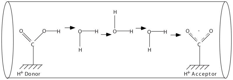
Schematics of a segment of proton conducting channel.
The described structures are different from those occurring in the membrane pores or ion channel, such as gramicidin and others [13,14,16,29,30]. Computer simulations of transport in proton conducting ion channels [9,11–14,31–37] have revealed a dramatic difference that a constrained environment of the channel can make, compared with the bulk transport. Earlier, a number of general qualitative ideas of how proton transport across biological membranes may occur have been developed [38–41]. The early concept of molecular wire [38] was challenged by Warshel [40], who developed the empirical valence bond (EVB) method, see e.g., [16], that provided the first computational approach to explore the issue quantitatively and arrived at the picture of localized charge diffusion. Later, the computational approaches have been significantly advanced, in particular by Voth and co-workers [12]. The mechanism of transport in specific proton conducting channels is still debated, however, see, e.g., [30], and is likely to be specific to a given biological system. If the state of hydrogen bonding network in a channel were the same as in liquid water, protons could randomly jump between water molecules at a rate of one jump per 1 ps, which would make the diffusion coefficient as high as 10−4 cm2/s. In protein channels, dynamics of water molecules is different from that in liquid state, and the corresponding rates of proton transport can be much slower than in the bulk [12].
Depending on the strength of hydrogen bonds along the conducting wire (which is defined, along with other factors, by the number of water molecules in the channel), proton transfer can occur either as a delocalized soliton [42–44] or as a localized (to a single hydrogen bond) charge. In the latter case, the transfer occurs as a random walk, or diffusion, of a localized charge along the wire, a process which involves many activated steps [15,16,23,24,26,36]. In the former case, the transition can be viewed as an activated single-step process, in which several protons shift coherently along the wire. In both types of proton transfer, the wire needs to be formed first, which is itself an activated process [32,45]. There is a finite lifetime associated with the wire. Proton transfer along the channel can therefore be described as a “gated” sequential reaction. The rate of such reaction can be written as
| (1.1) |
where is the rate of formation of the wire, τw is its life-time, and kPT is the rate of proton transfer along the assembled wire.
If PT transition occurs via delocalized soliton, then the transition itself is a fast process of the order of one period of nuclear vibration, in which all protons along the wire shift in a concerted way, while most of the reaction time the system “waits” until a necessary reorganization of the medium and the wire itself will occur. The rate of such a process is given by the generic expression
| (1.2) |
where τ0 ~ 10−12–10−13 s and Ea a is the activation energy for proton transfer.
On the other hand, if proton transfer along the wire occurs as a random walk of a localized charge, then the above formula (1.1) for kp is not applicable when proton diffusion is too slow. In this case the proton will never reach the acceptor site during the lifetime of a connected wire. Moreover, in this case the formation of a continuous wire along the whole channel is not necessary; here the proton transfer can be described simply as random walk along the channel, with some effective diffusion coefficient, and energy profile along the channel specific for a given redox state of the enzyme [1,36].
The formation of a continuous wire for a collective proton transfer is a process with high activation barrier, mainly due to a low entropy of the wire structure; on the other hand, if a continuous wire is not formed, the transport activation barrier is mainly due to energy cost of having a localized charge on a single water molecule (H3O+ or OH−) in a low dielectric protein medium. An important parameter that determines the type of the transfer mechanism is the number of water molecules in the channel. For example, in cytochrome c oxidase the mechanism of proton transport along a putative channel that connects Glu242 and propionate D of heme a3 (bovine heart notation) depends on whether three [21] or two [22] water molecules form the channel.
On the basis of structure of PRC, bc1 complex, and cytochrome oxidase, one cannot identify a unique organization of proton conducting channels, and therefore different mechanisms of proton transport appear to be possible. Two limiting cases of such mechanisms will be discussed below. To make analytical treatment possible, the models employed in the discussion involve some drastic simplifications of the real picture of the protein. Yet, such models (in addition to being interesting by themselves) are useful in providing a theoretical framework for the discussion of two conceptually different possibilities of transfer in real systems.
The collective effects in transport of protons along chains of hydrogen bonds have been discussed before in the context of solitons [44]. The soliton is a special collective localized excitation of the medium, which can propagate without dissipation and which exists due to nonlinearity of the system. The phenomenon is remarkably universal and appears in many areas of physics in a variety of forms. Solitons in molecular and condensed-matter physics were discovered in the mid 1970s by Davydov [46,47] and Krumhansl and Schrieffer [42]. Since then, the idea has expanded into many areas such as phase transitions [42], electron transport in conducting polymers [48,49], energy transfer in molecular and biological systems [43,50,51], proton transfer in hydrogen-bonded systems [44,52,53], and others [54].
The present paper utilizes some of the ideas developed in the soliton area and discusses their applications in the context of proton transfer reactions in bioenergetic enzymes. Our goal here is, by using tractable mathematical models, to clarify factors that determine the degree of delocalization of the transferring charge and to find a criterion for two limiting types of charge transfer described above.
II. MODEL HAMILTONIAN
We consider an idealized periodic chain of hydrogen-bonded water molecules shown schematically in Fig. 2(a). It will be assumed first that oxygen atoms are fixed in space; later this assumption will be relaxed (Sec. V). In a chain without defects, each oxygen atom has one proton, and in a minimum-energy configuration all protons are shifted to the left or to the right, as shown in the figure.
FIG. 2.

Distribution of protons (filled circles) in a hydrogen-bonded chain of water molecules; open circles are oxygen atoms and the curves are potential wells for protons. (a) No net charge in the chain. (b) Charge (−1) is localized to one molecule. (c) Charge is delocalized over several water molecules.
The potential-energy function for each of the protons consists of two parts. The first part is an effective interaction with two neighboring oxygen atoms, which is described by a symmetric double-well potential u(Q) shown in Fig. 3(a). The proton coordinate Q is measured from the midpoint between a pair of neighboring oxygen atoms. The u(Q) part is defined as energy per proton for a simultaneous shift of all protons in the chain, keeping the distances between them equal to those at equilibrium. At equilibrium, the protons are equidistant.
FIG. 3.

(a) Double-well potential for protons, u(Q). (b) Inverse potential −u(Q) and its stationary points.
The second part of the potential can be described as an effective interaction between the protons. If a proton in the chain is shifted from its equilibrium position, the associated energy increase consists of the u(Q) part, and an additional part which can be related to deviation of the interproton distances from their equilibrium values. This part can be described as a sum of pair-wise interactions χ(Qi − Qi+1). By definition, χ has a minimum when the distances between the protons are the equilibrium ones; hence a quadratic approximation for χ can be used.
The model Hamiltonian of the system therefore is
| (2.1) |
In a perfect chain at equilibrium, all protons are shifted to the right, Q0, or to the left position, −Q0, where the potential energy by definition is zero. (We should mention here that more realistic—and unfortunately more complicated—expressions for the effective Hamiltonian can be derived using the EVB approach [12,16]. Here we limit our discussion to a simplified analytically tractable model.)
Suppose now that one of the protons is missing or one additional proton is present in the chain. The first case corresponds to OH− and the second to H3O+ present in the system. The question is what are the equilibrium positions of the protons along the chain? Depending on the parameters of the potential-energy surface, the additional charge in the chain can be either localized to one water molecule (OH−) or (H3O+) or delocalized over several water molecules, as shown in Fig. 2. The second relevant question concerns the potential barrier for moving the charge along the chain.
The degree of delocalization is defined by the details of the potential surface of the system. To localize the charge on one molecular unit, as shown in Fig. 2(b), the energy cost is associated only with the increased distance between the pair of protons on both sides of the ion due to the interaction term . The rest of the system occupies one of the equilibrium positions ±Q0 and does not contribute to energy increase.
On the other hand, if the charge is delocalized along the chain, Fig. 2(c), the energy of proton-proton interactions is decreased because the pair-wise distances are now closer to their equilibrium values; however, the protons within the delocalization region are now shifted from their equilibrium positions toward the middle point between the neighboring oxygen atoms, and therefore their energy is increased, roughly u(0) per proton, due to potential u(Q). The equilibrium will be defined by the tradeoff between the strength of interaction constant k and the height of the barrier u(0).
Consider now a shift of the charge along the chain. If the charge is localized, the translational barrier is roughly . On the other hand, if the charge is delocalized, the translational barrier is decreased. The higher the degree of delocalization, the easier it is to move the charge along the chain.
To make the above considerations more quantitative, the continuum approximation is considered next. Instead of a discrete index n, a continuous variable x=an is introduced, where a is the distance between the molecules. The configuration of the system is described by Q(t,x), and the Hamiltonian for the system becomes
| (2.2) |
where the integration is extended over the whole length of the chain, ρ=m/a, κ=ka, V=u/a, Q̇ =dQ/dt, and ∇Q =dQ/dx.
The above Hamiltonian describes a one-dimensional “field” Q(t,x) and our problem becomes an elementary exercise in field theory. Below, a qualitative general analysis of the above Hamiltonian relevant to our problem will be presented. For some simple cases of V(Q) the problem can be solved exactly [44,48,52,53], Appendix A.
III. DELOCALIZATION LENGTH
Consider minimization of the potential energy of the system first. The energy expression is
| (3.1) |
When a negative charge is present in the system, the boundary conditions are Q=−Q0 for x → − ∞ and Q= +Q0 for x → +∞. The minimization can be done by standard variational techniques. We notice, however, that if coordinate x is treated as “time,” the above functional is equivalent to the action integral of a system with potential −V(Q) and mass κ. Thus, our problem is equivalent to finding a “trajectory” Q(x) in potential −V(Q), which satisfies the above boundary conditions, see Fig. 3(b). For these boundary conditions, the total mechanical energy of the system is zero,
| (3.2) |
From this we find
| (3.3) |
therefore the typical width of delocalization Ls can be found from the following equation:
| (3.4) |
Hence,
| (3.5) |
The trajectory Q(x) will qualitatively look like the one shown in Fig. 4.
FIG. 4.

(a) Distribution of proton displacements in a continuum model, u(Q). (b) Distribution of net charge corresponding to u(Q). Ls is the charge localization length.
It is instructive to obtain the delocalization length Ls in a different way. Namely, we approximate the actual trajectory, which satisfies Eq. (3.2) and qualitatively looks like the one shown in Fig. 4, by the following form:
| (3.6) |
where L is an adjustable parameter. Substitution of the above form into the expression for energy, Eq. (3.1), gives
| (3.7) |
The first term here represents the energy associated with proton-proton interactions. The smaller the charge delocalization length L, the larger this energy is. This interaction tends to align all protons in the chain evenly and make delocalization length as large as possible. The second term represents the energy of interaction with oxygen atoms. The larger delocalization L, the more protons will be shifted from equilibrium, toward the midpoint between neighboring oxygen atoms, where the potential V is largest. Hence this interaction tends to decrease L. The optimal length is a tradeoff between the two tendencies. Taking the derivative with respect to L, we arrive at the same expression for Ls as in Eq. (3.5).
IV. CHARGE DYNAMICS
The time-dependent solutions of the system are obtained from the action integral,
| (4.1) |
If a charge distribution propagates along the chain without changing the shape, the solutions should have the form
| (4.2) |
where f is the shape of charge distribution and v is the velocity of propagation. Now Q̇=−v∇Q. Substituting the above form into the expression for the action, we find
| (4.3) |
where T is the time interval and is the speed of sound in the proton sublattice (i.e., the maximum velocity at which a perturbation can propagate in the system). Except for a constant factor, the above expression coincides with energy functional (3.1) if we substitute
| (4.4) |
for κ. Finding the extremum of the above action is equivalent to minimizing Eq. (3.1) with κ= κ′. The later problem is already solved, and replacing κ with κ′ in Eq. (3.5) for the width of the moving charge, we find:
| (4.5) |
where is the width for zero velocity, Eq. (3.5). We see that there is a “Lorentzian” contraction of the delocalization length Ls.
Under normal conditions, the charge can move along the chain only with velocity v<c. The free propagation with speed v>c (“tachyon”) is possible only in unstable media, see Appendix A.
Consider now the kinetic energy of the moving charge K,
| (4.6) |
As expected, K is proportional to v2. We can introduce then an effective mass of the moving charge M by writing
| (4.7) |
Comparing this with the above expression for K and using the obtained expressions for Ls, Eqs. (3.5) and (4.5), we find
| (4.8) |
where M0 is the mass at zero velocity,
| (4.9) |
The analogy of the above expressions with the relativistic expressions for mass and length is quite remarkable. In Sec. VI we will discuss the microscopic meaning of the effective mass and velocity of propagation of charge distribution along the chain.
V. LATTICE RELAXATION
So far we considered oxygen atoms as being fixed in space. We now relax this assumption. Each oxygen atom is now considered to be moving in a quadratic potential around an equilibrium position in the chain, with a quadratic nearest-neighbor interaction,
| (5.1) |
where φn is the shift from equilibrium of the nth atom. The coupling with the protons is due to a term of the following form:
| (5.2) |
which describes the change in the oxygen-oxygen potential for protons u(Qn) as the distance between the nearest protons (φn+1 − φn) changes. It can also be interpreted as a shift of an equilibrium oxygen-oxygen distance as a function of the position of the shared proton. By its meaning, W is a positive function of Q, which is nonzero in the region of the barrier of u(Q), see Fig. 3(a). The effect of Hint is to decrease or increase the barrier between the two wells for a proton when the distance between the neighboring oxygen atoms is decreased or increased, respectively.
Going over to the continuum approximation, the Hamiltonian for the coupled system takes the form
| (5.3) |
The Lagrange equations of motion for this Hamiltonian are
| (5.4) |
| (5.5) |
The above equations describe the propagation of the charge and associated deformation of the chain. Assuming that the propagation occurs with velocity v, from the second equation for oxygen sublattice, we find
| (5.6) |
where is the speed of sound in the oxygen sublattice. From this equation, we can find φx for an arbitrary W and substitute it into the proton Eq. (5.4). As clear from Eq. (5.4) the propagation of charge will occur in the effective potential,
| (5.7) |
We see that qualitatively the effect of motion of oxygen atoms along the chain is formally reduced to a modification of the potential V(Q).
To simplify the formulas, we further assume that κO1 =0 and obtain
| (5.8) |
After substituting this into Eq. (5.4) the closed equation for proton sublattice takes the form
| (5.9) |
Taking into account that Q has the form of a propagating wave, f(x−vt), we find
| (5.10) |
Moreover after integration,
| (5.11) |
This equation has the same form as the one we considered for fixed oxygen atoms, Eq. (3.2), with the effective potential for protons
| (5.12) |
We see that the effect of adjustment of oxygen atoms to the charge in the chain is to decrease the barrier of V(Q), making Ṽ(0) smaller, and hence increasing the delocalization length Ls, see Eq. (3.5). The same qualitative result is obtained when the other limiting approximation is made in Eq. (5.6), namely, neglecting φxx and retaining the kO1φ term. Since Eq. (5.12) is obtained with an approximate treatment of Eq. (5.6), which is valid only for small velocity of propagation v, the velocity dependence of the effective potential (5.12) should be considered only qualitatively, namely, the delocalization length of the soliton wave is increased with an increase in the velocity of propagation of the soliton wave. [Taking v close to s, in Eq. (5.12), or even above s would be incorrect.]
It is clear, qualitatively, that the propagation of charge without dissipation of energy is only possible for velocity v less than the speed of sound in both the proton and oxygen sublattices: v<s and v<c. When the speed of propagation is close to the speed of sound in the sublattice, the continuum approximation breaks down, and a more detailed microscopic picture should be considered using exact solutions of Eqs. (5.4) and (5.5). As will be shown in Sec. VI, these limiting cases, although very interesting by themselves, unfortunately have very little to do with the proton transfer problem in protein.
VI. DISCUSSION
A. Microscopic parameters
The continuum approximation has been useful for the derivation of the analytical relations. We now wish to return to our original discrete representation and interpret the obtained results.
We begin from the expression for the delocalization length , Eq. (3.5), which can be written as
| (6.1) |
where a=2Q0 is the distance between the neighboring sites and n0 is the number of sites over which a resting charge is delocalized. The latter is written as
| (6.2) |
where
| (6.3) |
is the contraction energy due to proton-proton repulsion and
| (6.4) |
is the height of the barrier of u(Q).
When the charge moves with velocity v, the number of sites over which it is delocalized is
| (6.5) |
As the velocity v approaches the speed of sound c, the number of sites of delocalization shrinks to a minimum. The charge delocalization occurs when n0 ≫ 1. The contraction of the delocalization length with the increase in velocity of propagation should be understood as a limit n → 1 when v → c.
Consider the momentum of a moving charge. The number of protons involved in the motion is n=Ls/a, each moves between the two neighboring oxygen atoms with velocity vH = a/τ where τ=Ls/v is the time that the proton moves in the process. By definition, then
| (6.6) |
As seen, although the moving delocalized charge involves the motion of several protons, the overall momentum of the system is equal to that of a single proton moving with collective velocity v.
The kinetic energy of a moving charge is
| (6.7) |
where
| (6.8) |
We see that in contrast to the momentum relations, the kinetic energy is not equal to that of a single proton moving with velocity v. Instead, the effective mass appears, which is (1/n) th of the mass of the single proton. When the velocity approaches the maximum value c, the delocalization length reduces to one unit, the effective mass increases to its maximum value mH, the mass of a proton, and the kinetic energy becomes equal to that of a single proton.
Consider now the total mechanical energy of the system,
| (6.9) |
Recalling that the speed of sound c2= κ/ρ =ka2/mH, we find that the potential energy is
| (6.10) |
We can see again that the minimization of the above expression with respect to n gives for the optimal delocalization length . The potential energy of a delocalized resting charge is
| (6.11) |
Notice that for arbitrary ε1 and ε2,
| (6.12) |
The above potential energy is the minimum total mechanical energy for charge at rest, v=0. Consider now the maximum possible energy for v → c. In this case, in Eq. (6.9) n=1 and v=c. Therefore,
| (6.13) |
Recalling again that c2=ka2/mH =2ε1/mH we find that
| (6.14) |
Hence, the total energy of the charge varies in the range
| (6.15) |
From the above relations, we find that for an efficient delocalization, n ≫ 1, energy ε1 should be at least 1 order of magnitude larger than ε2. The evaluation of these two parameters for a specific system is discussed in Appendix B. It is clear that since these two energies are of the same origin, they can differ in maximum by 1 order of magnitude or so. Therefore, realistically for proton channels the maximum degree of delocalization can be
| (6.16) |
Given the structure of the channels, in which typically the same number of water molecules (three to five) are connecting the intermediate protonatable sites, we conclude that the charge transfer between the sites can occur via the charge delocalization process discussed above. The rate of proton transfer between the sites in this case will be given by formulas described in Sec. I. The overall transport then is a random walk over the intermediate protonation sites in the channel. The complete localization (n0 =1) case is also possible. In this case the jumps between the intermediate sites will require several activated transitions along the chain of water molecules connecting the sites. The overall transport in this case is also a random walk, which however is quite different from the former case. The two types of diffusion along the channel can be coupled to redox state of the enzyme, as described in Ref. [1].
B. Effects of disorder and temperature
It is already clear from the above discussion that the formal (continuous) theory of solitons has rather limited application to proton transfer in real proteins, since in proteins the charge is likely to be localized on just a few water molecules. Is it possible for such structures to propagate ballistically along a proton conducting channel, as in the formal continuous soliton theory discussed in Secs. IV and V? It appears that the effects of thermal and structural disorders and energy relaxation make such propagation impossible, further limiting the analogy between the solitary wave propagation and the proton transfer in a real system.
Indeed, taking the vibrational frequency of the protons to be (1 fs)−1 and the characteristic distances of proton transfer between the neighboring oxygen atoms to be roughly 1 Å, an estimate of the speed of sound in the protonic subsystem alone is 107 cm/s. On the other hand, assuming kinetic energy of the protonic soliton to be of the order of kilotesla, for T=300 K, the typical velocities of the solitons are roughly 105 cm/s. Thus, the effects of the velocity dependence of the delocalization length are not expected to be of great importance. Yet, even for such a high speed of propagation, assuming a typical vibrational energy relaxation time of 1 ps (the free propagation time), the mean-free path of a soliton is only of the order of 10 Å. Furthermore, if elasticity of the oxygen sublattice is taken into account, the effective speed of propagation (for the same kinetic energy of the order of kilotesla) is decreased, making the mean-free path even smaller, perhaps reduced to only to one or two water molecules. The same effects should be expected from the structural disorder of the chain along which the proton occurs. We conclude, therefore, that the ballistic (and coherent) soliton-like propagation of the delocalized charge structure in the real proton conducting system is impossible.
Given the above estimates, for a real system one is left with the following picture; the “solitons” should be understood in the sense of delocalized charge (positive H3O+ or negative OH−) over one to five water molecules; thermal disorder and energy relaxation makes ballistic propagation of such structures impossible; instead one should think of random walk of such structures along the proton conducting channel induced by thermal motions of the protein, as, e.g., in Ref. [26].
VII. CONCLUSIONS
Three qualitatively different cases of proton transfer along a proton conducting channel imbedded in the protein environment are possible. (a) The simplest case is when there are not enough water molecules in the channel to form a continuous chain. Such a case has been recently described in the context of cytochrome oxidase in Ref. [22]. In this case the transfer necessarily has to be via a localized charge. The individual water molecules have to carry the charge in the form of H3O+ or OH− between donor and acceptor groups via diffusion along the channel. The transfer activation barrier here is mainly due to energy costs of having a localized charge in a low dielectric medium of the protein.
(b) Water molecules in the channel form a continuous chain, as in an example described in Ref. [21]; however, because of geometrical constrains, the coupling along the chain is weak. In this case, the transferring charge is still localized on individual water molecules, and the transfer occurs via thermally activated hopping random walk of charge along the chain [25,26]. Due to partial hydrogen bonding, and a resulting local solvation of the charge, the activation barrier is expected to be lower than in the first case. The random walk along the channel is governed by the energy profile along the channel, which depends on the redox state of the enzyme [1]. The localized charge here can be formally described within a phenomenological model considered in this paper as a soliton localized on a single molecule, i.e., the soliton width Ls in this case is of the order of size of one water molecule [25,26].
(c) Water molecules form a continuous chain of hydrogen bonds with strong coupling. If such a chain existed as a stable entity of infinite length, one could apply directly the soliton model discussed in this paper. The soliton width Ls and charge delocalization in this case is much greater than one water molecule. [For the width estimate, one should take a soliton of the lowest thermal energy, i.e., the soliton with velocity v ≪ c, Eq. (6.5).] Realistically, in proteins, as discussed in Sec. VI, the water chain length between proton donor and acceptor groups is in the range of only three to five water molecules. In such a case we expect that under conditions of strong coupling and large soliton width, when an appropriate fluctuation in the chain and the environment occurs, the charge simply gets delocalized between donor and acceptor groups, along the whole length of the chain. The rate of charge transfer is described by formulas discussed in Sec. I. This type of transfer is qualitatively different from a random walk of a localized charge along the chain. The activation energy of charge transfer, Eq. (1.2), is expected to be lower than in the previous two cases.
Which of these three cases realizes in practice depends on the system? In cytochrome oxidase, for example, recent computer simulations in Ref. [22] predicted a situation of the A type; while simulations in Ref. [21] predicted a situation that is either B or C. The definitive answer as to which type of the transfer occurs in reality requires a detailed evaluation of the energetics of the charge transfer along the water channel [25,26,55]. The phenomenological model discussed in this paper can serve as a theoretical framework for rationalization of the numerical simulation results.
Acknowledgments
This work was supported by the National Science Foundation under Contract No. PHY 0646273.
APPENDIX A
(1) The exact solutions for the model can be generated from the following equation for energy:
| (A1) |
All solutions with boundary conditions discussed in text will have the form shown in Fig. 4. To find an analytically solvable potential, one can take any analytical form of the solution Q(x)and use the above equation to find V(Q). For example, for solution Q(x)=Q0 tanh(x/L) the potential is V(Q) =λ(1−(Q/Q0)2)2 where λ is a constant. For a given potential, multiple kink trajectories are also possible. They describe multiple charges in the chain.
(2) For velocity v>c the equation of motion has the form
| (A2) |
where
| (A3) |
Recall that x here is the evolution time. Thus, for v>c the potential in the equation of motion is V(Q) instead of −V(Q) for v<c. In this case, the “bounce” trajectory Q(x) can only originate at the top of the barrier Q=0, see Fig. 3(a). The trajectory will look as follows: it starts at the top of the barrier Q=0, then bounces left or right, and then returns back to the top of the barrier. In the x space the corresponding distribution of protons is as follows: all protons are located in the middle between two neighboring oxygen atoms, except for several protons within some delocalization interval Ls, in which protons are shifted to the left or to the right, according to Q(x). This structure can propagate with velocity v>c. This is clearly an artificial situation; in the chain, all protons initially are in the unstable position (top of the potential barrier) and the dynamics is such that they return to this position after a passage of the charge along the chain. Any perturbation can obviously destroy such an unstable state; therefore the v>c case is not realistic, although not impossible.
APPENDIX B
For a specific system, the parameters of the model can be evaluated as follows. By definition, the potential u(Q) is the energy per proton required to shift all protons in the chain, keeping their distances the same as in equilibrium, over distance Q. For a given periodic structure, this potential is obviously a symmetric double well. After the equilibration of protons, u(Q) then can be directly evaluated using methods of quantum chemistry.
The additional proton-proton interactions χ(Qi+1 − Qi) can be evaluated as the difference between the total potential energy U(Q) and u(Q) when a single proton (i) is shifted from its equilibrium position. By definition, in quadratic approximation, we have
| (B1) |
Keeping all protons at their equilibrium positions and varying the position of a single proton Qi, the interaction potential can be evaluated using the above relationship.
References
- 1.Stuchebrukhov AA. J Theor Comput Chem. 2003;2:91. [Google Scholar]
- 2.Cramer WA, Knaff DB. Energy Transduction in Biological Membranes. Springer; New York: 1990. [Google Scholar]
- 3.Wikstrom M. Curr Opin Struct Biol. 1998;8:480. doi: 10.1016/s0959-440x(98)80127-9. [DOI] [PubMed] [Google Scholar]
- 4.Berry EA, et al. Annu Rev Biochem. 2000;69:1005. doi: 10.1146/annurev.biochem.69.1.1005. [DOI] [PubMed] [Google Scholar]
- 5.Okamura MY, et al. Biochim Biophys Acta. 2000;1458:148. doi: 10.1016/s0005-2728(00)00065-7. [DOI] [PubMed] [Google Scholar]
- 6.Agmon N. Chem Phys Lett. 1995;244:456. doi: 10.1016/0009-2614(95)00906-k. [DOI] [PubMed] [Google Scholar]
- 7.Agmon N. J Phys Chem. 1996;100:1072. [Google Scholar]
- 8.Schmitt UW, Voth GA. J Chem Phys. 1999;111:9361. [Google Scholar]
- 9.Pomes R, Roux B. J Phys Chem. 1996;100:2519. [Google Scholar]
- 10.Vuilleumier R, Borgis D. J Phys Chem B. 1998;102:4261. [Google Scholar]
- 11.Decornez H, Hammes-Schiffer S. J Phys Chem A. 2000;104:9370. [Google Scholar]
- 12.Swanson JMJ, et al. J Phys Chem B. 2007;111:4300. doi: 10.1021/jp070104x. [DOI] [PMC free article] [PubMed] [Google Scholar]
- 13.Chen H, et al. Biophys J. 2007;92:46. doi: 10.1529/biophysj.106.091934. [DOI] [PMC free article] [PubMed] [Google Scholar]
- 14.Burykin A, Warshel A. Biophys J. 2003;85:3696. doi: 10.1016/S0006-3495(03)74786-9. [DOI] [PMC free article] [PubMed] [Google Scholar]
- 15.Warshel A. Computer Modeling of Chemical Reactions in Enzymes and Solutions. Wiley; New York: 1997. [Google Scholar]
- 16.Kato M, Pisliakov AV, Warshel A. Proteins. 2006;64:829. doi: 10.1002/prot.21012. [DOI] [PubMed] [Google Scholar]
- 17.Georgievskii Y, Medvedev ES, Stuchebrukhov AA. Biophys J. 2002;82:2833. doi: 10.1016/S0006-3495(02)75626-9. [DOI] [PMC free article] [PubMed] [Google Scholar]
- 18.Georgievskii Y, Medvedev ES, Stuchebrukhov AA. J Chem Phys. 2002;116:1692. [Google Scholar]
- 19.Smondyrev AM, Voth GA. Biophys J. 2002;82:1460. doi: 10.1016/S0006-3495(02)75500-8. [DOI] [PMC free article] [PubMed] [Google Scholar]
- 20.Popovic DM, Stuchebrukhov AA. FEBS Lett. 2004;566:126. doi: 10.1016/j.febslet.2004.04.016. [DOI] [PubMed] [Google Scholar]
- 21.Zheng X, et al. Biochim Biophys Acta. 2003;1557:99. doi: 10.1016/s0005-2728(03)00002-1. [DOI] [PubMed] [Google Scholar]
- 22.Wikström M, Verkhovsky MI, Hummer G. Biochim Biophys Acta. 2003;1604:61. doi: 10.1016/s0005-2728(03)00041-0. [DOI] [PubMed] [Google Scholar]
- 23.Olsson MH, Sharma PK, Warshel A. FEBS Lett. 2005;579:2026. doi: 10.1016/j.febslet.2005.02.051. [DOI] [PubMed] [Google Scholar]
- 24.Olsson MHM, Warshel A. Proc Natl Acad Sci USA. 2006;103:6500. doi: 10.1073/pnas.0510860103. [DOI] [PMC free article] [PubMed] [Google Scholar]
- 25.Olsson MH, et al. Biochim Biophys Acta. 2007;1767:244. doi: 10.1016/j.bbabio.2007.01.015. [DOI] [PMC free article] [PubMed] [Google Scholar]
- 26.Pisliakov AV, et al. Proc Natl Acad Sci USA. 2008;105:7726. doi: 10.1073/pnas.0800580105. [DOI] [PMC free article] [PubMed] [Google Scholar]
- 27.Quenneville J, Popovic DM, Stuchebrukhov AA. Biochim Biophys Acta. 2005;1757:1035. doi: 10.1016/j.bbabio.2005.12.003. [DOI] [PubMed] [Google Scholar]
- 28.Popovic DM, Stuchebrukhov AA. J Am Chem Soc. 2004;126:1858. doi: 10.1021/ja038267w. [DOI] [PubMed] [Google Scholar]
- 29.DeCoursey TE, Cherny VV. Isr J Chem. 1999;39:409. [Google Scholar]
- 30.Pinto LH, Lamb RA. J Biol Chem. 2005;281:8997. doi: 10.1074/jbc.R500020200. [DOI] [PubMed] [Google Scholar]
- 31.MaRrink S, Jahnig F, Berendsen HC. Biophys J. 1996;71:632. doi: 10.1016/S0006-3495(96)79264-0. [DOI] [PMC free article] [PubMed] [Google Scholar]
- 32.Pomes R, Roux B. Biophys J. 1996;71:19. doi: 10.1016/S0006-3495(96)79211-1. [DOI] [PMC free article] [PubMed] [Google Scholar]
- 33.Schumaker MF, Pomes R, Roux B. Biophys J. 2001;80:12. doi: 10.1016/S0006-3495(01)75992-9. [DOI] [PMC free article] [PubMed] [Google Scholar]
- 34.Brewer ML, Schmitt UW, Voth GA. Biophys J. 2001;80:1691. doi: 10.1016/S0006-3495(01)76140-1. [DOI] [PMC free article] [PubMed] [Google Scholar]
- 35.Zahn D, Brickmann J. Phys Chem Chem Phys. 2001;3:848. [Google Scholar]
- 36.Warshel A. Annu Rev Biophys Biomol Struct. 2003;32:425. doi: 10.1146/annurev.biophys.32.110601.141807. [DOI] [PubMed] [Google Scholar]
- 37.Smondyrev AM, Voth GA. Biophys J. 2002;83:1987. doi: 10.1016/S0006-3495(02)73960-X. [DOI] [PMC free article] [PubMed] [Google Scholar]
- 38.Nagle JF, Morowitz HJ. Proc Natl Acad Sci USA. 1978;75:298. doi: 10.1073/pnas.75.1.298. [DOI] [PMC free article] [PubMed] [Google Scholar]
- 39.Nagle JF, Tristram-Nagle SJ. J Membr Biol. 1983;74:1. doi: 10.1007/BF01870590. [DOI] [PubMed] [Google Scholar]
- 40.Warshel A. Photochem Photobiol. 1979;30:285. doi: 10.1111/j.1751-1097.1979.tb07148.x. [DOI] [PubMed] [Google Scholar]
- 41.Warshel A. Methods Enzymol. 1986;127:578. [Google Scholar]
- 42.Krumhansl JA, Schrieffer JR. Phys Rev B. 1975;11:3535. [Google Scholar]
- 43.Davydov AS. Solitons in Molecular Systems. Reidel; Dordrecht: 1991. [Google Scholar]
- 44.Bountis T. Proton Transfer in Hydrogen-Bonded Systems. Plenum; New York: 1992. [Google Scholar]
- 45.Brewer ML, Schmitt UW, Voth GA. Biophys J. 2001;80:1691. doi: 10.1016/S0006-3495(01)76140-1. [DOI] [PMC free article] [PubMed] [Google Scholar]
- 46.Davydov AS. J Theor Biol. 1973;38:559. doi: 10.1016/0022-5193(73)90256-7. [DOI] [PubMed] [Google Scholar]
- 47.Davydov AS. J Theor Biol. 1977;66:379. doi: 10.1016/0022-5193(77)90178-3. [DOI] [PubMed] [Google Scholar]
- 48.Su WP, Schrieffer JR, Heeger AJ. Phys Rev Lett. 1979;42:1698. [Google Scholar]
- 49.Heeger AJ, et al. Rev Mod Phys. 1988;60:781. [Google Scholar]
- 50.Davydov AS. Biology and Quantum Mechanics. Pergamon; New York: 1982. [Google Scholar]
- 51.Scott A. Phys Rep. 1992;217:1. [Google Scholar]
- 52.Antonchenko NY, Davydov AS, Zolotariuk AV. Phys Status Solidi B. 1983;115:631. [Google Scholar]
- 53.Zolotariuk AV, Spatschek KH, Laedke EW. Phys Lett. 1984;101A:517. [Google Scholar]
- 54.Bishop AR, Schneider T. Solitons and Condensed Matter Physics. Springer; Berlin: 1981. [Google Scholar]
- 55.Quenneville J, Stuchebrukhov AA. J Phys Chem B. 2009 in press. [Google Scholar]