

Abstract
Lesion analysis is a classic approach to study brain functions. Because brain function is a result of coherent activations of a collection of functionally related voxels, lesion‐symptom relations are generally contributed by multiple voxels simultaneously. Although voxel‐based lesion‐symptom mapping (VLSM) has made substantial contributions to the understanding of brain‐behavior relationships, a better understanding of the brain‐behavior relationship contributed by multiple brain regions needs a multivariate lesion‐symptom mapping (MLSM). The purpose of this artilce was to develop an MLSM using a machine learning‐based multivariate regression algorithm: support vector regression (SVR). In the proposed SVR‐LSM, the symptom relation to the entire lesion map as opposed to each isolated voxel is modeled using a nonlinear function, so the intervoxel correlations are intrinsically considered, resulting in a potentially more sensitive way to examine lesion‐symptom relationships. To explore the relative merits of VLSM and SVR‐LSM we used both approaches in the analysis of a synthetic dataset. SVR‐LSM showed much higher sensitivity and specificity for detecting the synthetic lesion‐behavior relations than VLSM. When applied to lesion data and language measures from patients with brain damages, SVR‐LSM reproduced the essential pattern of previous findings identified by VLSM and showed higher sensitivity than VLSM for identifying the lesion‐behavior relations. Our data also showed the possibility of using lesion data to predict continuous behavior scores. Hum Brain Mapp 35:5861–5876, 2014. © 2014 Wiley Periodicals, Inc.
Keywords: lesion‐symptom mapping, support vector regression, aphasia, total lesion volume control
INTRODUCTION
Localizing brain‐behavior relationships remains a key goal of cognitive neuroscience and clinical neurology. The relationship between lesion site(s) and behavior may be assessed using either functional or structural imaging. In functional neuroimaging (e.g., functional magnetic resonance imaging (fMRI)), brain activation is often presumed to indicate a causal role of the observed region in some cognitive process; however, the data generally admit a variety of other explanations, often including the possibility that the activity is epiphenomenal to the process of interest. Structural imaging‐based lesion‐symptom mapping (LSM) has long been used to study brain‐behavior relationships [Bates, 2003; Bendfeldt et al., 2012; Burges, 1998) and complements what can be learned from functional neuroimaging by providing high‐quality evidence that the integrity of a brain region is necessary for the normal performance of the measured function [Chatterjee, 2005; Fellows et al., 2005; Rorden and Karnath, 2004].
Voxel‐based lesion‐symptom mapping (VLSM) [Bates, 2003] represents an advance over the traditional overlap‐subtraction approach by providing a statistical way to assess brain‐behavior relationships. In VLSM, the brain‐behavior relationship is assessed on a voxel‐by‐voxel basis. In each voxel, patients with lesions are compared to those without lesions on the behavioral measure. The significance of the behavioral difference associated with lesion status is then inferred using a two‐sample t‐test or nonparametric methods such as permutation testing. Without using prior regions‐of‐interest (ROIs), VLSM provides a means to detect effects across the whole brain. However, as a univariate method, VLSM represents a suboptimal method for assessing the multivariate lesion‐symptom relationship. For example, it cannot consider data correlations among neighboring voxels although those correlations can be used to increase detection power [Kimberg et al., 2007]. Because VLSM is often based on dichotomized lesion data (either 1 [present] or 0 [absent]), which produces low variance at each voxel, hence limited power for predicting continuous behavioral performance (e.g., functional outcomes), although, that is, of great clinical interest.
Multivariate approaches have the potential to overcome these limitations in VLSM; however, multivariate lesion‐symptom mapping (MLSM) still remains new in the literature with few publications. In [Wang et al., 2012], we used a partial least square (PLS)‐based MLSM for simultaneously assessing lesion‐symptom relations in the semantic and phonological language domains. However, entering several behavioral scores into the same PLS model makes it difficult to associate each of the loading maps with a specific behavior measure. When only one behavior score is included, the PLS method is the same as VLSM. Chen et al. [Chen et al., 2008] proposed a voxel‐based Bayesian LSM method for detecting the nonlinear, multivariate associations between lesion locations and behavior measures but it was designed for the dichotomized behavior scores and provides no statistical inference for the association at each voxel. Smith et al., 2013 reported another multivariate lesion feature‐based behavior prediction study. By including ROI‐based multivariate lesion features in a support vector machine (SVM) [Cortes and Vapnik, 1995]‐based prediction model, they achieved very high accuracy for predicting behavior status (presence/absence of spatial neglect). Higher prediction power was showed by including more features such as the lesion statuses of different regions into the model. Using a combinatoric feature pruning approach, their method can also identify regions showing the most behavior (the presence of spatial attention deficits) prediction power. While an important advance, the two‐class SVM‐classification behavior status prediction requires a dichotomization of the continuous behavior statuses into a binary score, limiting its use in cases where performance grades continuously between two diagnoses, or between pathology and normality. In addition, the brute‐force combinatoric feature validating approach makes it an impractical tool for mapping the regional lesion‐behavior relationship if lesion feature is included from each voxel rather than ROIs. Logistic regression was used in [Kummerer et al., 2013] to evaluate the effects of controlling additional nuisance variables. Similar to the two‐class SVM classification, logistic regression can only predict a binary behavior status rather than a continuous one. In [Hope et al., 2013], high predicting accuracy was obtained by including both lesion volume and ROI‐based regional lesion status in a Gaussian Process model Regression. Different from the other studies, Hope et al. used continuous lesion maps rather than the binary ones.
In [Zhang et al. 2012], we piloted a machine learning regression, the support vector regression (SVR) [Vapnik, 1995], to predict language dysfunction using the spatial geometrical features (such as lesion volume, lesion size, maximum lesion pattern diameter, and lesion pattern surface area) of lesions. In this study, we extend that work into a SVR‐based MLSM (hereafter SVR‐LSM).
SVR is an extension of SVM [Cortes and Vapnik, 1995], which has been used in many brain imaging studies [Cox and Savoy, 2003; LaConte et al., 2005; Mourão‐Miranda et al., 2005; Wang et al., 2007] and lesion analysis as well [Smith et al., 2013]. While an SVM model is trained to optimally separate the input data by categories, an SVR model is trained to predict a continuous association variable (the behavioral measure in LSM) with high accuracy using all independent variables (here, all voxels' lesion statuses) [Smola and Schölkopf, 2004; Vapnik, 1995]. This multivariate (including all independent variables) input–output relationship mapping fits precisely the goals of MLSM.
To assess the feasibility and efficacy of SVR‐LSM, we first used synthetic data to evaluate SVR‐LSM and compare it to VLSM. The methods were compared for their performance in detecting lesion‐behavior correlations in spatially distributed regions with spatially varying contributions to the target lesion‐behavior association. We then evaluated SVR‐LSM using previously published lesion data and behavioral measures from patients with chronic, poststroke aphasia. The published data are from studies investigating what many believe to be a primary distinction between the processing of word meaning (semantics) and word sounds (phonology). For example, in the task of object naming, different cognitive operations are involved in producing a semantically appropriate word versus producing the word's phonological segments. To investigate the neural basis of semantic and phonological production, the researchers collected naming data from a large group of individuals with aphasia, from which they culled responses that qualified as “semantic errors” (apple named as “pear”) and those that qualified as “phonological errors” (apple named as “affen”). Analyses of semantic errors (SE) with VLSM consistently identified a region in the left anterior temporal lobe and, less consistently, prefrontal cortex [Schwartz et al., 2009; Schwartz et al., 2012; Walker et al., 2011]. The VLSM of phonological errors (PE) identified voxels concentrated in a region extending from frontal cortex to anterior parietal lobe [Schwartz et al., 2012]. This study used the SVR‐LSM method to investigate the lesions that give rise to each of these symptoms of naming impairment: SE and PE. The VLSM method was used, as well, with slight variations from the published studies for the purpose of enabling comparison with SVR.
THEORY
LSM Through Multiple Regression
Suppose the lesion maps are , each element representing a lesion map with voxels: , ( , is the number of subjects), and the behavior score is . LSM can be equivalently expressed as a multiple regression model:
| (1) |
where, are the fitting coefficients with representing the lesion‐behavior association strength at the th voxel , and are the fitting errors.
However, solving the multiple regression model is problematic because of the colinearity between neighboring voxels and also the under‐determinacy due to the much greater number of unknown variables in Eq. (1) (the number of voxels) than the number of observations (number of subjects). For example, a typical brain lesion map contains millions of voxels, but there are generally at most hundreds of participants (106 in this work). Directly solving such an extremely under‐determined problem is mathematically unstable, meaning that there will be an infinite number of solutions. To choose a practically meaningful and physically reasonable one, we need additional information to constrain the potential solutions.
Support Vector Regression
SVR is a machine‐learning‐based multiple regression method [Drucker et al., 1996]. SVR solves the aforementioned under‐determination problem by constraining the regression model to be “flat”: to get a minimum norm for the fitting coefficients. Because the regression model should still meet the original conditions, the model with a minimized fitting coefficient norm will be much less sensitive to noise or perturbation in the features and will be more stable for predicting future unknown data. Similar to SVM, SVR also takes a trade‐off between the fitting accuracy and prediction accuracy. An “insensitive” threshold is used to zero out training data fitting errors if they are less than the threshold. By releasing the fitting precision, SVR reduces the risk of over‐fitting. Both the model flatness and small fitting error insensitivity can result in better prediction accuracy for unknown data. When a linear fitting is not able to meet the criteria, SVR can also project the input data into a high‐dimensional feature space using a nonlinear transform so a linear model can be still built therein to fulfill the fitting criteria [Cortes and Vapnik, 1995]. The nonlinear transform depends on certain type of kernel functions. By means of a mathematical manipulation, the so‐called kernel trick [Vapnik, 1995], the real SVR learning process can avoid an explicit use of the underlying kernel function, so projection of input data into the high dimensional feature space can be skipped, thereby greatly simplifying the complex model learning process [Smola and Schölkopf, 2004].
For the th subject's lesion map and behavior score , SVR can be described by
| (2) |
where is the function transforming the independent variable (lesion data in this article) to a higher (even infinite) dimensional feature space, is the fitting coefficient in the high dimensional space, and is the fitting error. Except for the transform, this model is the same as that described in Eq. (1); and both operate in a map‐wise manner, in contrast with the voxel‐wise approach used in standard VLSM.
As described earlier, to overcome the under‐determination problem, SVR obtains the desirable solution by constraining the model to be “flat,” meaning that the norm (i.e., the length in the high dimensional feature space) of the fitting coefficient ( ) should be small. With this constraint, Eq. (2) can be expressed as a Lagrangian multiplier‐based minimization problem [Smola and Schölkopf, 2004]:
| (3) |
where, constant controls the trade‐off between the flatness and the tolerable fitting error [Hsu et al., 2010], and are slack variables to cope with losses outside of the soft margins, is an ε‐insensitive error function [Vapnik, 1995]:
| (4) |
Since the dimension of is very large, the constrained problem in Eq. (3) is more widely solved in its dual form:
| (5) |
where, is the Lagrangian, , , , and are Lagrange multipliers and are no less than 0. At the optimal solution, , , , and should be all zeroes. By expressing these properties in explicit equations, we can get a dual format of the optimization problem as described in Eq. (3):
| (6) |
By using a specific type of function (the so‐called kernel function) which can be expressed as an inner product: , Eq. (6) can be easily solved to get . The multiple regression model in Eq. (2) can then be got by
| (7) |
By solving the dual problem shown in Eq. (6), the number of unknown variables changes from (number of voxels of the lesion map) in Eq. (3) to (number of subjects) in Eq. (6). Since is much greater than ( ), solving the dual problem requires many fewer computations, and subsequently makes SVR a much more tractable problem. Procedures for finding the optimal solution using Eq. (6) are beyond the scope of this article, interested readers are referred to Cortes and Vapnik [1995] for details. Similar to SVM, the input variables (lesion maps in this article) with non‐zero coefficient are called support vectors. Since is unique to each training sample, it can be alternatively denoted by one variable for the simplicity of description.
In summary, SVR provides a practical solution to the under‐determined multiple regression problem by enforcing the model flatness and ignoring small fitting errors [Cortes and Vapnik, 1995]. A computationally efficient SVR can be implemented using its dual‐form.
SVR‐LSM
In SVR‐LSM, all lesion voxels are used as input to find a behavior predictive model. To explicitly utilizing the model for LSM, the model's parametric map (the predictive hyperplane) needs to be back projected into the input data space (the original brain space) to find the corresponding anatomical locations.
For SVR with a linear kernel , the feature space for the SVR predictive hyperplane is the same as that of the input data space (the 3D physical brain space), so that the lesion‐behavior relation at each voxel of the brain can be directly calculated as
| (8) |
For a nonlinear SVR, we need an inverse transform from the high or infinite dimensional feature space to the original image space. However, this inverse transformation is generally nontrivial and may not even solvable. To solve this problem, approximations have been taken in the so‐called “preimage” method [Arias et al., 2007; Dambreville et al., 2006; Kwok and Tsang, 2004; Mika et al., 1998]. But the preimage methods available in the literature involve computation‐intensive optimizations, which might not even converge. Based on the specific lesion data properties and assuming the widely used radial basis function (RBF) kernel is used, we showed in Appendix that a preimage method specific to SVR‐LSM can be obtained by using the following approximate back‐projection:
| (9) |
Note that in Eq. (9) is derived from a nonlinear SVR, which is different from the linear case in Eq. (8).
Through this back‐projection, we can get a lesion‐symptom map in the natural brain space, and use it for assessing regional brain‐behavior relationship. For clarity, this map was termed as the SVR‐LSM parametric map or the SVR‐LSM ‐map in following sections.
Another approach to get an input–output association map in the original input data space is “sensitivity mapping” [Zurada et al., 1994], which has been used in several studies for visualizing a nonlinear classifier [Kjems et al., 2002; Rasmussen et al. 2011; Strother et al., 2002]. Rather than taking a direct inverse transform of the kernel function, sensitivity mapping characterizes sensitivity of the model output (behavior scores in SVR‐LSM) to each input data dimension by calculating partial derivative of the output variable to the input variable in that dimension and then taking the sum over all input data dimensions. As we shown in Appendix, sensitivity mapping and the above preimage can be derived using first order Taylor expansion‐based approximation with slightly different mathematical manipulations. We thereby only considered the preimage approach in this study.
Statistical Inference for SVR‐LSM
While the prediction accuracy can be used to evaluate the SVR model, there is not a statistical approach for assessing the SVR predictive hyperplane and the associated SVR‐LSM ‐map. Similar to what is performed in SVM‐based fMRI data analysis [Mourão‐Miranda et al., 2005; Wang et al., 2007], permutation testing can be used to create a probability map to infer the regional lesion‐behavior relationship reflected by the SVR‐LSM ‐map. To be computationally efficient, the behavior data can be randomly shuffled to generate a series of pseudo SVR‐LSM ‐maps. At each voxel, the number of permutations whose pseudo values are greater than the one yielded from the nonpermuted data can be counted and divided by the number of permutations plus 1 to convert into a permutation probability. With this probability, we can test the null hypothesis that the SVR identified brain‐behavior association captured by the SVR‐LSM at each voxel is the same as that derived from random data. If the value is lower than a certain significance level (e.g., ), we can claim the association found in the current voxel to be a significant, true association. The same procedure is then repeated at all voxels to locate all behavior associated brain regions. A cluster extent threshold can be used to remove small suprathreshold clusters to further control false positive rate.
MATERIALS AND METHODS
Subjects
Patients with aphasia caused by left hemisphere stroke were recruited from the Neuro‐Cognitive Rehabilitation Research Patient Registry at the Moss Rehabilitation Research Institute [Schwartz et al., 2005] or the Center for Cognitive Neuroscience Patient Database at the University of Pennsylvania. Structural magnetic resonance imaging (MRI) or CT brain imaging was done under a protocol approved by the IRB at the University of Pennsylvania Medical School to obtain precise anatomical data. Participants were paid for their participation and reimbursed for travel and related expenses. Within all the subjects enrolled, 106 participants (43% female and 46% African American) qualified for this study. All of them were right‐handed before aphasia onset. Their mean age was 58 (range 26–79) and mean years of education was 14 (10–21). All were > 1 month post aphasia onset and living in the community. The great majority (86%) of them were chronic, that is, > 6 months post onset. The median postonset time was 21.5 months, and the mean post‐onset time was 50.6 months with a standard deviation of 66.6 months. The median total lesion volume was , and the mean total lesion volume was with a standard deviation of . The individual brain was normalized to the Montreal Neurological Institute “Colin27” brain template. Lesion data were manually segmented based on each patient's high resolution structural image and converted into binary maps. Details about image segmentation and normalization can be found in our previous publications using the same dataset [Schwartz et al., 2012].
Language Data
The PNT (Philadelphia Naming Test [Roach et al., 1996], available online: http://www.mrri.org/philadelphia-naming-test) tests basic‐level object naming capability with 175 object depictions from a variety of semantic categories. A standard coding scheme classifies each response as correct or one of five error types. Two error types were analyzed in this article. SE represent failure to select the right word based on its meaning. SE are real words that bear a semantic relation to the target; SE can be synonyms, category coordinates, superordinates, subordinates, or strong associates of the target (e.g., BOWL to “vase”; BENCH to “park”). According to cognitive models of anomia, SE can result from a failure to represent the concept correctly in semantic memory, or a failure to retrieve the correct word from the mental lexicon [e.g., Rapp and Goldrick, 2000]. PE represent failure to correctly retrieve and/or order the word's constituent phonemes. In this context, PE are nonwords that usually but not invariably bear a close resemblance to the target (e.g., GHOST to “goath”). For each participant, SE and PE were expressed as a proportion of total trials (175) to create the variables SE and PE, respectively.
Image Acquisition and Lesion Segmentation
Ninety‐four participants received research 3.0‐T MRI (n = 56) or CT (n = 38) brain scans. Twelve additional participants declined scanning; for those subjects, recent clinical scans (8 CT, 4 MRI) with clearly delineated lesion boundaries were substituted in the lesion tracing procedure. Lesions were manually segmented on the structural image by a trained technician or experienced neurologist, both of whom were blinded to the behavioral data [please refer to details in Schwartz et al., 2009]. The lesion overlap map for the 106 qualified participants at the left hemisphere is shown in Figure 1a.
Figure 1.

Lesion overlap map and predefined ROIs for generating synthetic scores in simulations. a: Lesion overlap map of 106 subjects. Colorbar on the right indicates the number of lesion subjects. The text above each slice indicates the spatial location of the sagittal slice in the MNI space. b: Three predefined ROIs used for generating the synthetic score in simulations. c: The correlation map between the lesion status of each voxel and the total lesion volume. Correlation coefficients to the total lesion volume for ROI 1∼3 are 0.7301, 0.7002, and 0.2942, respectively. [Color figure can be viewed in the online issue, which is available at http://wileyonlinelibrary.com.]
VLSM Method with Simple Regression
Only voxels lesioned in patients were included in the analysis. For each language measure, SE and PE, a VLSM analysis was performed by running a simple regression analysis, with the lesion status as the independent variable and the behavior score as the dependent variable, at each voxel for PE and SE separately. The fitting coefficient map (beta‐map) was converted into a t‐map using SPM (http://www.fil.ion.ucl.ac.uk/spm/, Wellcome Institute of Imaging Neuroscience, London, UK). 1,000 permutations were performed by randomly permuting the behavior scores (SE or PE). The lesion versus no lesion contrast map (VLSM t‐map) obtained from the genuine data order was compared to those obtained by permuting the data at each voxel, and the number of permutations yielding higher VLSM t‐value than the genuine one was divided by 1,001 to get the permutation P‐value.
SVR‐LSM
The same lesion data were used in the SVR‐LSM analysis. Only voxels lesioned in patients were included in the analysis and formed a valid voxel mask. For each subject, the lesion statuses of all voxels in the valid voxel mask were grouped into one column vector. As a general preprocessing step in SVR, each subject's lesion data vector was normalized to have a unit norm, that is, the square root of the sum of squared elements for each vector equals to 1. It is important to note that this normalization process also serves as a direct total lesion volume control procedure (hereafter dTLVC). It differs from the approach previously adopted [Karnath et al., 2004; Schwartz et al., 2012], in which the total lesion volume effects were directly regressed out from the behavior scores. The normalized vectors from all participants were combined into a feature matrix with rows representing different subjects. The language scores were also inputted into a column vector and normalized. libSVM [Chang and Lin, 2011] with an epsilon‐SVR model was used to estimate the SVR hyperplane with an RBF kernel. A grid searching approach was used to assess the effects of the two SVR parameters, and , on SVR‐LSM. 168 different combinations of and with changing from 1 to 80, and γ changing from 0.1 to 30 were evaluated for both the synthetic data and the real SE and PE data. The behavior score prediction accuracy as well as the reproducibility of SVR‐LSM were collected to find the optimal SVR parameters. Prediction accuracy was measured by the mean correlation coefficient between predicted scores and testing scores with 40 five‐fold cross‐validations. SVR‐LSM was evaluated by another 40 times subset analysis, each with a randomly selected 85 subjects, and the correlation coefficient between any two SVR‐LSM ‐maps from different subsets was calculated. The mean of those correlations was used as a reproducibility index.
Simulations
SVR‐LSM was evaluated with synthetic lesion‐behavior relations inserted into 3 a priori cubic ROIs (shown in Fig. 1b) based on the actual lesion data from the 106 subjects. The ROIs were defined in the left hemisphere, where the number of lesioned brains at each voxel was at least 10. Each ROI was a cube. The ROIs were positioned at different locations to produce different correlations between their lesion volume ratios and the total lesion volume. This specification was used to evaluate the effects of total lesion volume control on LSM using both VLSM and SVR‐LSM. The correlations were 0.7301, 0.7002, and 0.2942 for ROI 1, 2, and 3, respectively.
The artificial brain‐behavior relations were generated based on a weighted sum of lesion volume ratios of the three ROIs using the following equation:
| (10) |
where, is the artificial score for the i‐th subject, is the weight of the k‐th ROI to the artificial score, is the lesion volume ratio of the k‐th ROI in the i‐th subject, which was calculated as the ratio of the number of lesion voxels to the total number of voxels in the th ROI, and is a function for simulating the artificial linear brain‐behavior relationship . Four different sets of weights: {1, 1, 1}, {1, 2, 1}, {1, 1, 2}, and {2, 1, 1} (the three numbers in the brackets are weights for ROI 1, 2, and 3, respectively) for the three ROIs were used to generate pseudobehavior scores with differently weighted contributions from the three ROIs.
Both VLSM and SVR‐LSM were then used to localize the predefined lesion‐symptom regions with and without dTLVC. Model performance was quantified using the receiver operator characteristic (ROC) method [Metz, 1978]. To calculate the ROC curves, both the SVR‐LSM ‐map and the VLSM t‐map were thresholded with values descending from the maximum to the minimum of the corresponding map values. At each threshold, a true positive rate (proportion of suprathreshold voxels within the ROIs) and a false positive rate (proportion of suprathreshold voxels outside the ROIs) were calculated. The ROC curves were obtained by plotting the true positive rates versus the false positive rates for all possible thresholds for each type of methods. A better performing LSM method should yield a ROC curve that is closer to the true positive axis while farther away from the false positive axis. The area under the curve (AUC) was calculated to quantify the performance, where a larger AUC means better performance.
To provide a statistical comparison for the lesion‐behavior relation detection performance of VLSM and SVR‐LSM, the above simulations were repeated 100 times. During each simulation, three nonoverlapping cubic ROIs were randomly generated within the mostly lesioned area ( subjects were lesioned) as shown in Figure 1a. The AUC values of all simulations were then compared using paired t‐test for LSM with or without lesion control separately.
SE and PE prediction using SVR‐LSM
While the primary purpose of this study was to investigate the use of SVR for LSM, a secondary question that has yet been explored much in the literature was whether the SVR model would be useful for predicting the continuous SE and PE scores using the whole brain lesion map. The prediction accuracy was evaluated using 40 times fivefold cross‐validations. Each validation used a randomly selected lesion and behavior data from 4/5 of the entire patients to train the SVR model, and the rest 1/5 subjects for testing.
RESULTS
Training Parameters
Figure 2 shows the prameter evaluation results for the RBF kernel‐based SVR‐LSM. Similar to what reported in [Rasmussen et al., 2012], prediction accuracy and reproducibility changed with the two parameters in an opposite maner: prediction accuracy goes down when reproducibility goes up. While there is no golden standard for choosing the optimal values, they were chosen to have a compromised high reproducibility and prediction accuracy. All six figures (Fig. 2a–f) shows that prediction and reproducibility did not change dramatically when C was between 30 and 80. Since larger C will induce overfitting, we chose 30 as the optimal value for C. We selected for the synthetic behavior data and for both SE and PE analysis based on the above mentioned criterium because the reproducibility for the synthetic behavior data increased more rapidly than that for the real scores (SE and PE) along with the increasing of .
Figure 2.
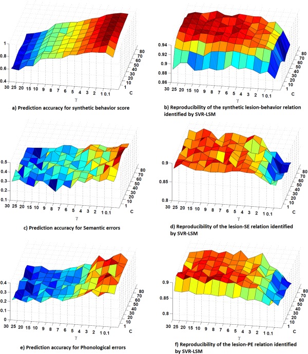
SVR parameter evaluation results. a, c, and e: are the cross‐validation prediction accuracy for synthetic score, SE‐ and PE versus lesion association analysis, respectively; b, d, and f: show the reproducibility of the SVR‐LSM β‐map for the three datasets, respectively. [Color figure can be viewed in the online issue, which is available at http://wileyonlinelibrary.com.]
Simulation Results
Detection of the synthetic lesion‐behavior relations
Figure 3 shows the results of VLSM and SVR‐LSM for detecting the spatially uniformly weighted (with the weight set {1, 1, 1}) synthetic linear lesion‐behavior associations. The parametric maps of VLSM and SVR‐LSM were thresholded separately to make the number of suprathreshold voxels inside and outside the ROIs equal the total number of voxels in the three ROIs, to directly compare both the true positive and false positive voxels. When no dTLVC was used, all voxels in ROI 3 and most voxels in ROI 1 went undetected by both methods, although both methods successfully detected most voxels in ROI 2 (Fig. 3a,c). Without dTLVC, both methods yielded many false positive voxels in the area between ROI 1 and ROI 2. Since the lesion status of voxels between ROI 1 and 2 was highly correlated with the total lesion volume, as indicated by the lesion overlap map in Figure 1c, it appears that total lesion volume had a strong effect on LSM results. When dTLVC was applied, SVR‐LSM showed much increased sensitivity in ROI 1 and 3 (Fig. 3d). VLSM showed relatively increased sensitivity for ROI 1, but it produced false postive voxels in areas that were not revealed without dTLVC (Fig. 1c).
Figure 3.
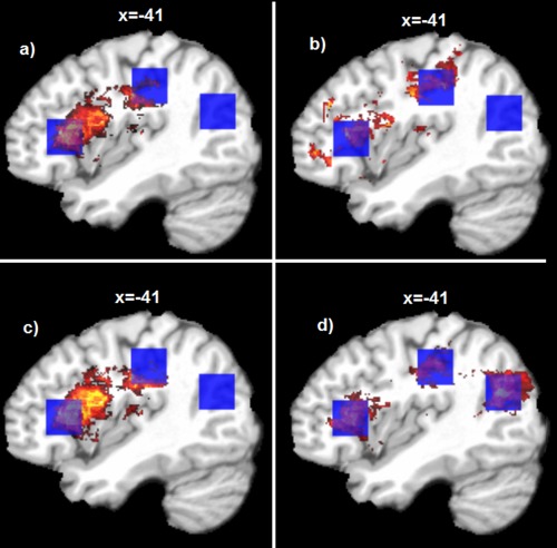
LSM results for the synthetic linear brain‐behavior relations. a and c: are results of VLSM and SVR‐LSM methods without dTLVC; b and d are results of VLSM and SVR‐LSM methods with dTLVC. The blue cubes indicate a priori ROIs used for inserting the pseudo brain‐behavior relations. Only the sagittal slice at x = −41 mm in the MNI space are shown; the seemingly different number of voxels in different figures was caused by different distributions of the suprathreshold voxels across different sagittal slices. [Color figure can be viewed in the online issue, which is available at http://wileyonlinelibrary.com.]
Figure 4 shows the ROC curves of VLSM and SVR‐LSM methods for the same synthetic data used above. Curves that are closer to the upper left corner mean higher true positive detection rate at the same level of false positive detection rate. Consistent with results shown in Figure 3, SVR‐LSM with dTLVC yielded the best ROC performance as indicated by the AUC value. Without dTLVC, VLSM and SVR‐LSM methods achieved similar ROC performance with slightly higher AUC in SVR‐LSM.
Figure 4.
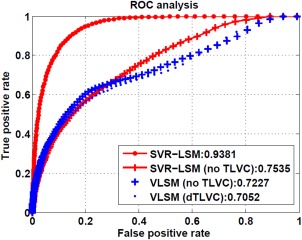
ROC curves of SVR‐LSM and VLSM with or without dTLVC for detecting the synthetic brain‐behavior relationship. The numbers in the legend are the AUC value for different methods. [Color figure can be viewed in the online issue, which is available at http://wileyonlinelibrary.com.]
Statistical performance of SVR‐LSM for the synthetic lesion‐behavior relation detection
Figure 5 shows box plots of the AUC values of VLSM and SVR‐LSM without or with lesion volume control. When no lesion volume control was applied (Fig. 5a), VLSM and SVR‐LSM showed no significant performance difference ( 0.5428). When lesion volume control was applied (Fig. 5b), SVR‐LSM showed significantly better AUC performance ( ).
Figure 5.
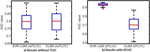
Statistic comparison results for the AUC values of VLSM and SVR‐LSM without dTLVC (a) and with dTLVC (b). [Color figure can be viewed in the online issue, which is available at http://wileyonlinelibrary.com.]
LSM for detecting spatially nonuniformly weighted lesion‐behavior relations
Table 1 lists the AUC values of the ROC curves as well as the average value (for SVR‐LSM) and average z‐scores (for VLSM, converted from the t‐scores before averaging) for LSM simulations using the aforementioned spatially nonuniformly weighted lesion‐behavior relations. For most of simulations listed there, SVR‐LSM produced larger AUC values than VLSM with or without dTLVC. Using dTLVC, the SVR‐LSM values in the three ROIs showed a high coincidence with the a priori specified weights for generating the synthetic data.
Table 1.
Lesion‐behavior relation detection results of SVR‐LSM and VLSM using different synthetic lesion‐behavior relations generated with different relation weights for the a priori ROIs
| Weights for ROIs | {1, 1, 1} | {1, 2, 1} | {1, 1, 2} | {2, 1, 1} | ||
|---|---|---|---|---|---|---|
| SVR‐LSM (dTLVC) | AUC value | 0.9405 | 0.8961 | 0.8713 | 0.9036 | |
| Mean β‐value | ROI‐l | 4.2782 | 3.034 | 2.1938 | 6.1869 | |
| ROI‐2 | 4.8871 | 6.8202 | 2.8001 | 3.4520 | ||
| ROI‐3 | 5.2198 | 4.0095 | 5.8688 | 3.5301 | ||
| VLSM (dTLVC) | AUC value | 0.7052 | 0.6185 | 0.8072 | 0.6478 | |
| Mean z‐value | ROI‐l | 4.4511 | 3.8026 | 3.5386 | 5.6773 | |
| ROI‐2 | 4.4520 | 6.5614 | 2.9188 | 3.7504 | ||
| ROI‐3 | 1.4795 | 0.3437 | 3.4840 | 0.8626 | ||
| SVR‐LSM (no dTLVC) | AUC value | 0.7574 | 0.6793 | 0.8322 | 0.7188 | |
| Mean β‐value | ROI‐l | 7.4194 | 5.9060 | 6.7722 | 7.8349 | |
| ROI‐2 | 8.1215 | 8.6247 | 6.7665 | 6.8357 | ||
| ROI‐3 | 3.8664 | 2.1706 | 6.5550 | 2.7985 | ||
| VLSM (no dTLVC) | AUC value | 0.7227 | 0.6403 | 0.8421 | 0.6829 | |
| Mean z‐value | ROI‐l | 7.4312 | 6.5513 | 5.9898 | 8.6966 | |
| ROI‐2 | 8.1426 | 9.5399 | 5.8576 | 7.3014 | ||
| ROI‐3 | 3.4899 | 2.1608 | 5.8486 | 2.7169 | ||
LSM for SE
Figure 6a–c show the nonthresholded VLSM t‐map, the SVR‐LSM map, and the suprathreshold permutation probability maps ( , cluster size > 50) for the lesion‐SE relations, respectively. dTLVC was applied for both VLSM and SVR‐LSM. The nonthresholded parametric maps of VLSM and SVR‐LSM were very similar, with a map‐wise correlation coefficient of 0.9401. This confirms the previously reported association between SE production and damage in inferior frontal gyrus (Brodmann area 44, 45, and 47) as well as damage in the left middle temporal gyrus (Brodmann area 21) [Schwartz et al., 2009].
Figure 6.
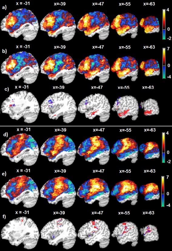
Lesion‐symptom relation mapping results using 106 Aphasia patients' data, both VLSM and SVR‐LSM implements include dTLVC to control the effect of total lesion volume. a–c: are for lesion‐SE relations, and d–f are for lesion‐PE relations. a: The non‐thresholded VLSM t‐map; b: the non‐thresholded SVR‐LSM map; c: thresholded (p ≤0.001, cluster size > 50) permutation probability maps of the lesion‐SE relations detected by VLSM (blue color) and SVR‐LSM (red color); d: The non‐thresholded VLSM t‐map; e: The non‐thresholded SVR‐LSM map; f: thresholded (p≤0.001, cluster size > 50) permutation probability maps of the lesion‐PE associations detected by VLSM (blue color) and SVR‐LSM (red color). The text above each slice indicates the spatial location of the sagittal slice in the MNI space. [Color figure can be viewed in the online issue, which is available at http://wileyonlinelibrary.com.]
LSM for PE
Figure 6d–f are the nonthresholded VLSM t‐map, SVR‐LSM map of the lesion‐PE relations, and the thresholded permutation testing results ( , cluster size>50), respectively. VLSM and SVR‐LSM (both with dTLVC) produced very similar lesion‐PE association results with a map‐wise correlation coefficient of 0.8709. Both methods identified robust lesion‐PE associations in central, supra‐Sylvian cortices of the left hemisphere, involving mainly pre‐ and postcentral gyrus (Brodmann areas 4/6 and 1/2/3, respectively) and the supramarginal gyrus; and both yielded few suprathreshold voxels in the auditory‐ and linguistic‐sensitive cortices of the posterior superior and middle temporal gyri.
Lesion‐Based Behavior Prediction Accuracy
With the five‐fold cross‐validations, SVR‐LSM showed a mean prediction accuracy of 0.10 (R square: the square of the Pearson correlation coefficient between the predicted value and the true scores, ) and 0.11 (R square: the square of the Pearson correlation coefficient, ) for SE and PE, respectively. The total lesion volume showed a correlation coefficient of 0.3021 and 0.1687 for SE and PE, respectively.
DISCUSSION
We report a SVR‐based MLSM method, SVR‐LSM. Rather than assessing the brain‐behavior relation at each voxel separately as in the standard VLSM, SVR‐LSM identifies the entire lesion‐behavior association pattern simultaneously. This multivariate learning process and the nonlinear transform for projecting the input data into a high dimensional feature space both take account of the spatial correlations between different lesion voxels into account. The resultant multivariate lesion‐symptom relation map reflected by the model hyperplane is more influenced by voxels with strong lesion‐symptom associations. Meanwhile, the weak lesion‐symptom relations that might be caused by noise are suppressed, resulting in improved lesion‐behavior detection sensitivity and reduced false positive rate. Our simulations clearly showed the benefit of using SVR‐LSM for detecting the synthetic lesion‐behavior relationship, in terms of higher sensitivity and specificity than VLSM. This scenario is similar to making statistical inference for a cluster of correlated voxels.
Lesion volume control is an important component of LSM. In previous studies, lesion volume has been regressed out from the behavior scores [Karnath et al., 2004; Schwartz et al., 2012] to control its effects. Because local lesion statuses are correlated with total lesion volume and both contribute to brain dysfunctions, regressing out lesion volumes from the behavior scores will inevitably suppress the relation between local lesion status and behavior score. One consequence is that lesions in regions that are highly correlated with total lesion volume may be treated as total lesion volume effects and inappropriately excluded from the final results. To avoid this over‐correction, a better approach is to apply volume control directly to the lesion data similar to the volume control used in the voxel‐based morphometry [Ashburner and Friston, 2000]. This dTLVC turns out to be a routine preprocessing step in SVR. Our simulations showed that dTLVC plays a significant role in SVR‐LSM. First, SVR without dTLVC could not reach the optimal performance, as expected. Second, the synthetic data had a strong volume effect, so the false positive rate was high in voxels adjacent to the prior ROIs. Removing volume effects greatly suppressed those false positives, due to the multivariate processing. In the analysis of actual patient data, SVR‐LSM with dTLVC identified reliable brain‐SE relations in a region (left lateral prefrontal cortex) that in our earlier studies had failed to survive correction for total lesion volume control [Walker et al., 2011; see also Schwartz et al., 2009]. We maintain that the previously used method, which corrected for lesion volume by regressing it out of the behavioral measure (SE), may be excessively conservative.
Using previously published aphasia patient data, SVR‐LSM showed much higher sensitivity than VLSM for identifying both brain‐SE and brain‐PE relations. Major significant clusters found by SVR‐LSM confirmed and extended our previous findings with VLSM. In particular, the SVR analysis of SE identified a cluster in the mid‐to‐anterior part of the left middle temporal gyrus and another in the left lateral prefrontal cortex [Schwartz et al., 2009; Walker et al., 2011]. The former area is strongly linked to verbal semantic processing [Mesulam et al., 2013; Patterson et al., 2007], the latter to executive control of semantic retrieval [Bookheimer, 2002; Schnur et al., 2009]. Therefore, it may be that lesions in these areas cause SE for different reasons. Regardless, it can be inferred from the present findings that these temporo‐frontal areas form a deficit‐contributing network for SE. This is because unlike VLSM, the multivariate LSM picks up the coherence (correlation) of the different areas, as well as their independent contributions.
The SVR‐LSM analysis of PE confirmed our previous findings with VLSM associating PE in naming with lesions in premotor and anterior parietal cortices, and not Wernicke's area [Schwartz et al., 2012; see also Cloutman et al., 2009; Foundas et al., 1998]. Such convergence of results from two very different lesion mapping techniques inspires confidence in the results. This is important, because the results for PE were not predictable from current theorizing. The identified brain‐PE relationships go against the long‐held view that PE in naming are symptomatic of impaired retrieval of abstract or auditory‐based phonemic representations stored in posterior temporal cortices [Dell et al., 1997; Indefrey and Levelt, 2004; Wilson, et al., 2009; Wernicke, 1874/1969], aligning better with newer models featuring close interdependence of phonological and sensori‐motor processes in production [Hickok, 2012].
Figure 6 suggests little if any overlap between the SE and PE associated regions. Since the data that entered into these separate analyses came from the same group of patients and the very same task (picture naming), it appears likely that semantic and phonological operations in word production are subserved by different brain systems, the former localized to temporo‐frontal regions of the left hemisphere, the latter to fronto‐parietal regions.
Parameter determinations for nonlinear SVR are important but nontrivial. For output prediction, small allows a better prediction performance, large yields small fitting errors for the training data; small allows a better model flexibility (wider kernel and smoother SVR hyperplane). However, higher prediction accuracy does not mean a better spatial pattern interpretation for the model predictive hyperplane [Rasmussen et al., 2011]. In [Rasmussen et al., 2011], the pattern reproducibility across various subsets of the entire samples was suggested as an additional index for determining parameters. In this study, we took a balance between prediction accuracy and model reproducibility to find the optimal values for the two involved parameters. While the optimal values were determined using the 106 patients' data, similar values should work for other data too as we empirically tested (data not shown). Nevertheless, a reasonable range for and of [1∼50] and [0.5∼10] respectively can be used as the searching range. For using SVR to predict behavior scores, the parameters should be separately tuned using the prediction accuracy as the optimization objective function during cross‐validations. While we only reported a prediction accuracy using the parameters selected for a best LSM detection, additional experiments using parameters tuned for a better prediction accuracy did the job by increasing the SE prediction accuracy (R‐square) from 0.10 to 0.18 though that is still low.
Nonlinear SVR was used in SVR‐LSM. While a linear SVR could still be used, nonlinear SVR provides more flexibility for model selection to get either better prediction accuracy or better association localization. Additional data analysis showed (Fig. 7) that linear SVR was suboptimal as compared to the nonlinear SVR even with the optimized cost parameter C for linear SVR ( ). But remapping the nonlinear SVR model back into the input data space has been a challenge. Based on the lesion data properties, we derived an approximate preimage method, which turns out to be dual to the “sensitivity mapping” approach. Additional data analysis (data not shown) showed that SVR‐LSM ‐maps were nearly the same as the sensitivity maps derived from the sensitivity mapping process.
Figure 7.
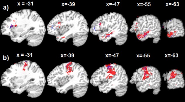
Thresholded (p , cluster size > 50) permutation probability maps of the nonlinear SVR‐LSM (Red) and linear SVR‐LSM (Blue). a: results for SE‐lesion relations, b: results for PE‐lesion relations. The text above each slice indicates the spatial location of the sagittal slice in the MNI space. [Color figure can be viewed in the online issue, which is available at http://wileyonlinelibrary.com.]
Multiple comparison correction is a big topic in neuroimaging and LSM because of its over‐conservation even after considering the spatial correlations between neighboring voxels. In SVR‐LSM, the lesion‐symptom associations at all voxels are identified simultaneously rather than being pursued as independent events, so there are no multiple comparisons involved for getting the association parametric map. While SVR does not provide a statistical framework for inferring the model hyperplane, an approximate approach is using cross validations to find the prediction accuracy and its probability. For inferring the regional effects (thresholding the SVR‐LSM sensitivity map), it is still not clear whether a multiple comparison correction should be applied or not. A compromise approach might be getting a conditional probability for each voxel by combining the probability of the model prediction power and the permutation probability. Nevertheless, this will be an interesting topic in future study.
While the major focus of this study was to exploit the utility of SVR for LSM, we also provided the first evidence that multivariate lesion‐behavior relationship patterns can be useful for predicting continuous behavioral scores.
In conclusion, SVR‐LSM with dTLVC is a useful method for lesion symptom analysis with higher sensitivity and specificity than standard VLSM. It is also potentially useful for using brain lesion status to predict behavioral performance in clinical practice.
SVR WITH A LINEAR KERNEL
For SVR model with a linear kernel , the model in Eq. (7) could be written as
| (A1) |
Since linear kernel does not transform the lesion data into high dimension, the coefficient for each voxel's lesion status in the brain image space could be expressed by , which is identical to the sensitivity map for a linear kernel [Rasmussen et al., 2011].
SVR WITH THE RBF MODEL
The RBF kernel function can be described by the inner product of and
| (A2) |
With the trained coefficients ( ), the lesion‐brain model can be written as
| (A3) |
where e is Euler's number ( ). Since the total lesion volume of subjects is typically very large (typically hundreds of thousands to even millions of lesion voxels), the normalized lesion data value and are very small. We can then use the first Taylor expansion‐based approximation of ( means approximation) and get
| (A4) |
Because lesion data are normalized to have a norm of 1, . Since , the greater than 3‐order terms are very small and can be then removed. Considering all these facts and we can get:
| (A5) |
and
| (A6) |
The other type of approximate preimage expression can be derived by approximating Eq. (A2) with its first order Taylor expansion:
| (A7) |
Where
| (A8) |
which is exactly the same as “sensitivity mapping” [Rasmussen et al., 2011; Zurada et al., 1994]. This sensitivity mapping formula is known to have a sign cancellation problem [Rasmussen et al., 2011]. But it is less problematic for lesion data because there are large amount of subjects do not have lesion at many voxels, so they would not contribute to the summation process. Additionally those subjects showing large distance from the evaluated one ( will have very minor contribution because the exponential term becomes close to 0. A quadratic formula can still be used if there is severe sign cancellation.
REFERENCES
- Arias P, Randall G, Sapiro G (2007): Connecting the out‐of‐sample and pre‐image problems in kernel methods. In: IEEE Computer Society Conference on Computer Vision and Pattern Recognition, pp. 1–8, Minneapolis, Minnesota, USA.
- Ashburner J, Friston KJ (2000): Voxel‐based morphometry—The methods. NeuroImage 11:805–821. [DOI] [PubMed] [Google Scholar]
- Bates E (2003): Voxel‐based lesion‐symptom mapping. Nat Neurosci 6:448–450. [DOI] [PubMed] [Google Scholar]
- Bendfeldt K, Klöppel S, Nichols TE, Smieskova R, Kuster P, Traud S, Mueller‐Lenke N, Naegelin Y, Kappos L, Radue EW, Borgwardt SJ (2012): Multivariate pattern classification of gray matter pathology in multiple sclerosis. Neuroimage 60:400–408. [DOI] [PubMed] [Google Scholar]
- Bookheimer SY (2002): Functional MRI of language: New approaches to understanding the cortical organization of semantic processing. Annu Rev Neurosci 25:151–188. [DOI] [PubMed] [Google Scholar]
- Burges CJC (1998): A tutorial on support vector machines for pattern recognition. Data Mining Knowledge Discov 2:121–167. [Google Scholar]
- Chang CC, Lin CJ (2011): LIBSVM: A library for support vector machines. ACM Trans Intell Syst Technol 2:27:1–27:27. [Google Scholar]
- Chatterjee A (2005): A madness to the methods in cognitive neuroscience? J Cogn Neurosci 17:847–849. [DOI] [PubMed] [Google Scholar]
- Chen R, Hillis AE, Pawlak M, Herskovits EH (2008): Voxelwise Bayesian lesion‐deficit analysis. NeuroImage 40:1633–1642. [DOI] [PMC free article] [PubMed] [Google Scholar]
- Cloutman L, Gottesman R, Chaudhry P, Davis C, Kleinman JT, Pawlak M, Herskovits EH, Kannan V, Lee A, Newhart M, Heidler‐Gary J, Hillis AE (2009): Where (in the brain) do semantic errors come from?. Cortex 45:641–649. [DOI] [PMC free article] [PubMed] [Google Scholar]
- Cortes C, Vapnik V (1995): Support‐vector network. Mach Learn 20:273–297. [Google Scholar]
- Cox DD, Savoy RL (2003): Functional magnetic resonance imaging (fMRI) “brain reading”': Detecting and classifying distributed patterns of fMRI activity in human visual cortex. NeuroImage 19:261–270. [DOI] [PubMed] [Google Scholar]
- Dambreville S, Rathi Y, Tannenbaum A (2006): Statistical shape analysis using kernel PCA. In: IS&T/SPIE Symposium on Electrical Imaging, 6064(B), San Jose, California, USA.
- Dell GS, Schwartz MF, Martin N, Saffran EM, Gagnon, DA (1997): Lexical access in aphasic and nonaphasic speakers. Psychol Rev 104:801–838. [DOI] [PubMed] [Google Scholar]
- Drucker H, Burges CJC, Kaufman L, Burges CJC, Kaufman L, Smola A, Vapnik V (1996): Support vector regression machines. Adv Neural Inf Process Syst (NIPS) 9:155–161.
- Fellows LK, Heberlein AS, Morales DA, Shivde G, Waller S, Wu DH (2005): Method matters: An empirical study of impact in cognitive neuroscience. J Cogn Neurosci 17:850–858. [DOI] [PubMed] [Google Scholar]
- Foundas A, Daniels SK, Vasterling JJ (1998): Anomia: Case studies with lesion localization. Neurocase 4:35–43. [Google Scholar]
- Hickok, G (2012): Computational neuroanatomy of speech production. Nat Rev Neurosci 13:135–145. [DOI] [PMC free article] [PubMed] [Google Scholar]
- Hope TMH, Seghier ML, Leff AP, Pricea CJ (2013): Predicting outcome and recovery after stroke with lesions extracted from MRI images. Nueroimage Clin 2:424–433. [DOI] [PMC free article] [PubMed] [Google Scholar]
- Hsu C‐W, Chang C‐C, Lin C‐J(2010): A practical guide to support vector classification. Bioinformatics 1:1–16. [Google Scholar]
- Indefrey P, Levelt WJM (2004): The spatial and temporal signatures of word production components. Cognition 92:101–144. [DOI] [PubMed] [Google Scholar]
- Karnath HO, Berger MF, Kuker W, Rorden C (2004): The anatomy of spatial neglect based on voxelwise statistical analysis: A study of 140 patients. Cereb Cortex 14:1164–1172. [DOI] [PubMed] [Google Scholar]
- Kimberg DY, Coslett HB, Schwartz MF (2007): Power in voxel‐based lesion‐symptom mapping. J Cogn Neurosci 19:1067–1080. [DOI] [PubMed] [Google Scholar]
- Kjems U, Hansen LK, Anderson J, Frutiger S, Muley S, Sidtis J, Rottenberg D, Strother SC (2002): The quantitative evaluation of functional neuroimaging experiments: Mutual information learning curves. Neuroimage 15:772–786. [DOI] [PubMed] [Google Scholar]
- Kummerer D, Hartwigsen G, Kellmeyer P, Glauche V, Mader I, Kloppel S, Suchan J, Karnath HO, Weiller C, Saur D. (2013). Damage to ventral and dorsal language pathways in acute aphasia. Brain 136:619–629. [DOI] [PMC free article] [PubMed] [Google Scholar]
- Kwok JT‐Y, Tsang IW‐H(2004): The pre‐image problem in kernel methods. IEEE Trans Neural Networks 15:1517–1525. [DOI] [PubMed] [Google Scholar]
- LaConte S, Strother S, Cherkassky V, Anderson J, Hu X. (2005): Support vector machines for temporal classification of block design fMRI data. NeuroImage 26:317–329. [DOI] [PubMed] [Google Scholar]
- Mesulam M, Wieneke C, Hurley R, Rademaker A, Thompson CK, Weintraub S, Rogalski EJ (2013): Words and objects at the tip of the left temporal lobe in primary progressive aphasia. Brain 136:601–618. [DOI] [PMC free article] [PubMed] [Google Scholar]
- Metz CE (1978): Basic principles of ROC analysis. Semin Nucl Med 8:283–298. [DOI] [PubMed] [Google Scholar]
- Mika S, Schölkopf B, Smola A, Müller K‐R, Scholz M, Rätsch G (1998): Kernel PCA and de‐noising in feature spaces. Adv Neural Inf Process Syst 11:536–542. [Google Scholar]
- Mourão‐Miranda J, Bokde ALW, Born C, Hampel H, Stetter M (2005): Classifying brain states and determining the discriminating activation patterns: Support vector machine on functional MRI data. NeuroImage 28:980–995. [DOI] [PubMed] [Google Scholar]
- Patterson K, Nestor PJ, Rogers TT (2007): Where do you know what you know? The representation of semantic knowledge in the human brain. Nat Rev Neurosci 8:976–987. [DOI] [PubMed] [Google Scholar]
- Rapp B, Goldrick M (2000): Discreteness and interactivity in spoken word production. Psychol Rev 107:460–499. [DOI] [PubMed] [Google Scholar]
- Rasmussen PM, Madsen KH, Lund TE, Hansen LK (2011): Visualization of nonlinear kernel models in neuroimaging by sensitivity maps. NeuroImages 55:1120–1131. [DOI] [PubMed] [Google Scholar]
- Rasmussen PM, Hansen LK, Madsen KH, Churchill NW, Strother SC (2012): Model sparsity and brain pattern interpretation of classification models in neuroimaging. Pattern Recognit 45:2085–2100. [Google Scholar]
- Rasmussen PM, Schmah T, Madsen KH, Lund TE, Yourganov G, Strother SC, Hansen LK (2012): Visualization of Nonlinear Classification Models in Neuroimaging‐Signed Sensitivity Maps. In: Proceedings of International Conference on Bio‐inspired Systems and Signal Processing (Biosignal 2012). pp. 254–263, Vilamoura, Algarve, Portugal. [Google Scholar]
- Roach A, Schwartz MF, Martin N, Grewal RS, Brecher A (1996): The Philadelphia naming test: Scoring and rationale. Clin Aphasiol 24:121–133. [Google Scholar]
- Rorden C, Karnath HO (2004): Using human brain lesions to infer function: A relic from a past era in the fMRI age? Nat Rev Neurosci 5:813–819. [DOI] [PubMed] [Google Scholar]
- Schnur TT, Schwartz MF, Kimberg DY, Hirshorn E, Coslett HB, Thompson‐Schill SL (2009): Localizing interference during naming: Convergent neuroimaging and neuropsychological evidence for the function of Broca's area. Proc Natl Acad Sci USA 106:322–327. [DOI] [PMC free article] [PubMed] [Google Scholar]
- Schwartz MF, Brecher A, Whyte JW, Klein MG (2005): A patient registry for cognitive rehabilitation research: A strategy for balancing patients' privacy rights with researchers' need for access. Arch Phys Med Rehabil 86:1807–1814. [DOI] [PubMed] [Google Scholar]
- Schwartz MF, Kimberg DY, Walker GM, Faseyitan O, Brecher A, Dell GS (2009): Anterior temporal involvement in semantic word retrieval: VLSM evidence from aphasia. Brain 132:3411–3427. [DOI] [PMC free article] [PubMed] [Google Scholar]
- Schwartz MF, Faseyitan O, Kim J, Coslett HB (2012): The dorsal stream contribution to phonological retrieval in object naming. Brain 135:3799–3814. [DOI] [PMC free article] [PubMed] [Google Scholar]
- Smith DV, Clithero JA, Rorden C, Karnath H‐O(2013): Decoding the anatomical network of spatial attention. Proc Natl Acad Sci USA 110:1518–1523. [DOI] [PMC free article] [PubMed] [Google Scholar]
- Smola AJ, Schölkopf B (2004): A tutorial on support vector regression. Stat Comput 14:199–222. [Google Scholar]
- Strother S, Anderson J, Hansen L, Kjems U, Kustra R, Sidtis J, Frutiger S, Muley S, LaConte S, Rottenberg D (2002): The quantitative evaluation of functional neuroimaging experiments: The NPAIRS data analysis framework. Neuroimage 15:747–771. [DOI] [PubMed] [Google Scholar]
- Vapnik VN (1995): The Nature of Statistical Learning Theory. Springer, New York, NY, USA. [Google Scholar]
- Walker GM, Schwartz MF, Kimberg DY, Faseyitan O, Brecher A, Dell GS, Coslett HB. (2011). Support for anterior temporal involvement in semantic error production in aphasia: New evidence from VLSM. Brain Lang 117:110–22. [DOI] [PMC free article] [PubMed] [Google Scholar]
- Wang Z (2009): A hybrid SVM‐GLM approach for fMRI data analysis, NeuroImage 46:608–615. [DOI] [PMC free article] [PubMed] [Google Scholar]
- Wang Z, Childress AR, Wang J, Detre JA (2007): Support vector machine learning‐based fMRI data group analysis. NeuroImage 36:1139–1151. [DOI] [PMC free article] [PubMed] [Google Scholar]
- Wang Z, Faseyitan OK, Kimberg DY, Coslett HB, Schwartz MF (2012): Lesion‐based Language Deficit Localization and Prediction Using Partial Least Square (PLS) Analysis. In: Annual Meeting of the Organization for Human Brain Mapping (OHBM), Beijing, China, June 11.
- Wernicke C (1874/1969): The aphasic symptom complex: A psychological study on a neurological basis, Cohn and Weigert Cohen RS, Wartofsky MW, editors. Boston Studies in the Philosophy of Science, Vol. 4 Boston: Reidel, Breslau. [Google Scholar]
- Wilson SM, Isenberg AL, Hickok G (2009): Neural correlates of word production stages delineated by parametric modulation of psycholinguistic variables, Hum Brain Mapp 30:3596–3608. [DOI] [PMC free article] [PubMed] [Google Scholar]
- Zhang Y, Kimberg DY, Coslett HB, Schwartz MF, Wang Z (2012): Language Deficit Prediction Using Brain Lesion Geometry Feature‐based Support Vector Regression. In: Annual Meeting of the Organization for Human Brain Mapping (OHBM), Beijing, China, June 11.
- Zurada J, Malinowshi A, Cloete I (1994): Sensitivity Analysis for Minimization of Input Data Dimension for Feedforward Neural Networks. In: IEEE International Symposium on Circuits and System, 6:447–450, London, England, UK.