A Nth-order linear algorithm for extracting diffuse correlation spectroscopy blood flow indices in heterogeneous tissues

Abstract

Conventional semi-infinite analytical solutions of correlation diffusion equation may lead to errors when calculating blood flow index (BFI) from diffuse correlation spectroscopy (DCS) measurements in tissues with irregular geometries. Very recently, we created an algorithm integrating a Nth-order linear model of autocorrelation function with the Monte Carlo simulation of photon migrations in homogenous tissues with arbitrary geometries for extraction of BFI (i.e., αD_B). The purpose of this study is to extend the capability of the Nth-order linear algorithm for extracting BFI in heterogeneous tissues with arbitrary geometries. The previous linear algorithm was modified to extract BFIs in different types of tissues simultaneously through utilizing DCS data at multiple source-detector separations. We compared the proposed linear algorithm with the semi-infinite homogenous solution in a computer model of adult head with heterogeneous tissue layers of scalp, skull, cerebrospinal fluid, and brain. To test the capability of the linear algorithm for extracting relative changes of cerebral blood flow (rCBF) in deep brain, we assigned ten levels of αD_B in the brain layer with a step decrement of 10% while maintaining αD_B values constant in other layers. Simulation results demonstrate the accuracy (errors < 3%) of high-order (N ≥ 5) linear algorithm in extracting BFIs in different tissue layers and rCBF in deep brain. By contrast, the semi-infinite homogenous solution resulted in substantial errors in rCBF (34.5% ≤ errors ≤ 60.2%) and BFIs in different layers. The Nth-order linear model simplifies data analysis, thus allowing for online data processing and displaying. Future study will test this linear algorithm in heterogeneous tissues with different levels of blood flow variations and noises.

Near-infrared (NIR) diffuse correlation spectroscopy (DCS),¹ also known as diffusing-wave spectroscopy,^2,3 has been developed and validated for noninvasive and continuous monitoring of relative changes of blood flow (rBF) in a variety of in vivo tissues with a depth up to centimeters.¹ A blood flow index (BFI) is usually generated by fitting DCS autocorrelation function to analytical solutions of correlation diffusion equation under simple tissue boundaries.^4–7 Among these boundaries, the semi-infinite geometry is commonly used due to its simplicity, which assumes the tissue measured to have a large volume with flat surface. However, our previous studies found that semi-infinite approximation leads to calculation errors of BFI in tissues with small volume and large curvature.⁸

Very recently, we created an algorithm integrating a Nth-order linear model of autocorrelation function with the Monte Carlo simulation of photon migrations in homogenous tissues for the extraction of BFI and rBF.⁹ Results from computer simulations and in vivo experiments in homogenous tissue models with different volumes and geometries demonstrate the accuracy and robustness of the linear algorithm. However, most of biological tissues are not homogenous. The purpose of this study is to extend the capability of the Nth-order linear algorithm for extracting BFI values in heterogeneous tissues with arbitrary volumes and geometries. After deriving a Nth-order linear algorithm used in heterogeneous tissues, we compared it with the semi-infinite homogenous solution for extracting BFI and rBF in a computer model of adult head with heterogeneous tissue layers of scalp, skull, cerebrospinal fluid (CSF), and brain.^10,11

The DCS principle and instrumentation can be found elsewhere.^4,12,13 Briefly, long-coherence NIR light (650 to 900 nm) is launched by a laser into the tissue via a source fiber. After transporting/scattering through the tissue, photons are collected by avalanche photodiodes via single-mode fibers placed millimeters to centimeters away from the source fiber. An autocorrelator board reads the detected photons and calculates light intensity autocorrelation function, from which the normalized electric field temporal autocorrelation function g₁(τ) of the detected light is derived. g₁(τ) is dependent on the motion of moving scatterers (primarily red blood cells) in the tissue. For homogeneous tissues, g₁(τ) (modulus value) can be determined by^8,13

$$g_1(\tau )=\frac{〈E\left(0\right)E^{*}(\tau )〉}{〈{\left|E\left(0\right)\right|}^2〉}={\int }_0^{\infty }P\left(s\right)\text{exp}\hspace{0.17em}(–\frac{1}{3}{k}_0^2⟨\Delta r^2(\tau )⟩\frac{s}{l^{*}})ds.$$ (1)

Here, P(s) is the normalized distribution of detected photon pathlength s, k₀ is the wave vector magnitude of the light in the medium, l^* is the photon random-walk step length, which is equal to 1/μ_s′ (μ_s′ is the reduced scattering coefficient), and τ is the delay time of autocorrelation function. 〈Δr²(τ)〉 is the mean-square-displacement of the moving scatterers. Based on flow models adopted, 〈Δr²(τ)〉 can have different forms. The diffuse motion model with a form of 〈Δr²(τ)〉 = 6D_Bτ was found to fit experimental data well over a wide range of tissues,⁴ where D_B (unit: cm²/s) is the effective diffusion coefficient. A factor α is added to 〈Δr²(τ)〉 (i.e., 〈Δr²(τ)〉 = 6αD_Bτ) because not all scatterers are “moving” in the tissue;⁴ α is the ratio of “moving” scatterers to the total scatterers. The combined term αD_B is referred to as BFI in the tissue, and the relative change in BFI (i.e., BFI/BFI_baseline) as rBF.¹²

Also, the unnormalized electric field temporal autocorrelation function G₁(τ) = 〈E(0)E^*(τ)〉 satisfies the correlation diffusion equation^4,13

$$\left(D{\nabla }^2-v{\mu }_a-\frac{1}{3}v{\mu }_s^{\prime }{k}_0^2〈\Delta r^2(\tau )〉\right)G_1\left(\overrightarrow{r},\tau \right)=-vS\left(\overrightarrow{r}\right).$$ (2)

Here, v is the light speed in the medium, D ≈ v/3 ${\mu }_s^{\prime }$ is the medium photon diffusion coefficient, μ_a is the medium absorption coefficient, and $S(\overrightarrow{r})\hspace{0.17em}\hspace{0.17em}$ is continuous-wave isotropic source. The analytical solution of Eq. (2) with semi-infinite geometry is often used to extract αD_B in homogenous tissues.⁴

For heterogeneous tissues consisting of n tissue types (e.g., scalp, skull, CSF, brain) with the assumption that 〈Δr²(τ)〉 is homogeneous within each tissue type,^10,11 Eq. (1) can be rewritten as

$$\begin{array}{c}{g}_1(\tau )={\int }_0^{\infty }P(s_1,\mathrm{...},s_n)\text{exp}\hspace{0.17em}(–\frac{1}{3}\sum _{i=1}^n{k}_0^2\left(i\right)⟨\Delta r_i^2(\tau )⟩\frac{s_i}{l_i^{*}})d(s_1,\mathrm{...},s_n)\\ ={\int }_0^{\infty }P(s_1,\mathrm{...},s_n)\text{exp}(-2\sum _{i=1}^n{k}_0^2\left(i\right)\alpha D_B\left(i\right)s\left(i\right){\mu }_s^{\prime }\left(i\right)\tau \left)\mathrm{d}\right(s_1,\mathrm{...},s_n).\end{array}$$ (3)

Similar to the linear algorithm for homogenous tissues,⁹ $g_1(\tau )$ can be expressed as the form of N-order Taylor polynomial

$$g_1(\tau )=g_1\left(0\right)+g_1^{\left(1\right)}\left(0\right)\tau +\sum _{k=2}^N\frac{g_1^{\left(k\right)}\left(0\right)}{k!}{\tau }^k+\frac{g_1^{(N+1)}(\xi ){\tau }^{N+1}}{(N+1)!}\hspace{0.17em},\hspace{1em}(0<\xi <\tau ).$$ (4)

Here,

$$g_1(0)={\int }_0^{\infty }P(s_1,\mathrm{...},s_n)d(s_1,\mathrm{...},s_n)=1.$$ (5)

Let

$$M(s_1,\mathrm{...},s_n)=2\sum _{i=1}^n{k}_0^2(i)\alpha D_B(i)s(i){\mu }_s^{\prime }\left(i\right)\hspace{0.17em}\hspace{0.17em}.$$ (6)

From Eq. (3), we have

$$g_1(\tau )={\int }_0^{\infty }P(s_1,\mathrm{...},s_n)\hspace{0.17em}\text{exp}(-M(s_1,\mathrm{...},s_n)\tau )d(s_1,\mathrm{...},s_n),$$ (7)

$$g_1^{(k)}(\tau )={\int }_0^{\infty }P(s_1,\mathrm{...},s_n){[-M(s_1,\mathrm{...},s_n)]}^k\hspace{0.17em}\text{exp}[-M(s_1,\mathrm{...},s_n)\tau ]d(s_1,\mathrm{...},s_n)\hspace{0.17em}\hspace{0.17em}(k\ge 1).$$ (8)

When τ = 0

$${g_1}^{(k)}(0)={\int }_0^{\infty }P(s_1,\mathrm{...},s_n){[-M(s_1,\mathrm{...},s_n)]}^{k}d(s_1,\mathrm{...},s_n).$$ (9)

Combining Eqs. (3), (4), and (9), we have

$$\begin{array}{c}{g}_1(\tau )-\text{1-}{\displaystyle \sum _{k=2}^N\frac{{\displaystyle {\int }_0^{\infty }P(s_1,\mathrm{...},s_n){[-M(s_1,\mathrm{...},s_n)]}^k}d(s_1,\mathrm{...},s_n)}{k!}{\tau }^k}=\tau {\displaystyle {\int }_0^{\infty }P(s_1,\mathrm{...},s_n)[-M(s_1,\mathrm{...},s_n)]}d(s_1,\mathrm{...},s_n)\\ +\frac{{\displaystyle {\int }_0^{\infty }P(s_1,\mathrm{...},s_n){[-M(s_1,\mathrm{...},s_n)]}^{N+1}\exp [-M(s_1,\mathrm{...},s_n)\xi ]}d(s_1,\mathrm{...},s_n)}{(N+1)!}{\tau }^{N+1},(0<\xi <\tau )\text{.}\end{array}$$ (10)

When τ is sufficient small, the second term on the right side of Eq. (10) can be ignored. The first-order (N = 1) and Nth-order (N > 1) approximations are thus derived from Eq. (10), respectively

$$g_1(\tau )-1=\tau {\int }_0^{\infty }P(s_1,\mathrm{...},s_n)[-M(s_1,\mathrm{...},s_n)]d(s_1,\mathrm{...},s_n).$$ (11)

$$\begin{array}{c}{g}_1(\tau )-1–\sum _{k=2}^N\frac{{\int }_0^{\infty }P(s_1,\mathrm{...},s_n){[-M(s_1,\mathrm{...},s_n\left)\right]}^{k}d(s_1,\mathrm{...},s_n)\hspace{0.17em}\hspace{0.17em}\hspace{0.17em}\hspace{0.17em}}{k!}{\tau }^k\\ =\tau {\int }_0^{\infty }P(s_1,\mathrm{...},s_n)[-M(s_1,\mathrm{...},s_n\left)\right]d(s_1,\mathrm{...},s_n).\end{array}$$ (12)

When utilizing Monte Carlo simulations of photon migrations in heterogeneity tissues and assuming a total of Q photons are detected, Eqs. (11) and (12) become

$$\begin{array}{c}{g}_1(\tau )-1=-\tau \sum _{p=1}^{Q}w(p)(2\sum _{i=1}^n{k}_0^2(i)\alpha D_B(i)s(i,p){\mu }_s^{\prime }\left(i\right))\\ =\tau \sum _{i=1}^n-2(\sum _{p=1}^{Q}w(p)k_0^2(i)s(i,p){\mu }_s^{\prime }\left(i\right))\alpha D_B(i).\end{array}$$ (13)

$$\begin{array}{c}{g}_1(\tau )-1-\sum _{k=2}^N\frac{{\sum _{p=1}^{Q}w\left(p\right)\left(-2\sum _{i=1}^n{k}_0^2\left(i\right)\alpha D_B\left(i\right)s(i,p){\mu }_s^{\prime }\left(i\right)\hspace{0.17em}\right)}^k}{k!}{\tau }^k\hspace{0.17em}\hspace{0.17em}\\ =\tau \sum _{i=1}^n\left(\sum _{p=1}^Q-2w\left(p\right)k_0^2\left(i\right)s(i,p){\mu }_s^{\prime }\left(i\right)\right)\alpha D_B\left(i\right).\end{array}$$ (14)

Here, we define w(p) = P(s₁,s₂,…,s_n) to present the normalized distribution of pth photon detected. s(i, p) is the photon pathlength of the pth photon in ith tissue type.

Equations (13) and (14) contain n unknowns of BFIs (i.e., αD_B(i), i = 1,2,…,n). To solve these unknowns, it is generally required to collect multiple DCS correlation functions at n S-D separations.

For jth (j = 1,…,n) S-D separation, Eqs. (13) and (14) become

$$\begin{array}{c}{g}_1(\tau ,j)-1=-\tau \sum _{p=1}^{Q}w(p,j)(2\sum _{i=1}^n{k}_0^2(i)\alpha D_B(i)s(i,p,j){\mu }_s^{\prime }\left(i\right))\\ =\tau \sum _{i=1}^n(\sum _{p=1}^Q-2w(p,j)k_0^2(i)s(i,p,j){\mu }_s^{\prime }\left(i\right))\alpha D_B(i)=\tau \sum _{i=1}^{n}A(i,j)\hspace{0.17em}\alpha D_B(i).\end{array}$$ (15)

$$\begin{array}{c}{g}_1(\tau ,j)-1-\sum _{k=2}^N\frac{{\sum _{p=1}^{Q}w(p,j)\left(-2\sum _{i=1}^n{k}_0^2\left(i\right)\alpha D_B\left(i\right)s(i,p,j){\mu }_s^{\prime }\left(i\right)\hspace{0.17em}\right)}^k}{k!}{\tau }^k\\ =-\tau \sum _{p=1}^{Q}w(p,j)\left(2\sum _{i=1}^n{k}_0^2\left(i\right)\alpha D_B\left(i\right)s(i,p,j){\mu }_s^{\prime }\left(i\right)\hspace{0.17em}\right)\\ =\tau \sum _{i=1}^n\left(\sum _{p=1}^Q-2w(p,j)k_0^2\left(i\right)s(i,p,j){\mu }_s^{\prime }\left(i\right)\right)\alpha D_B\left(i\right)=\tau \sum _{i=1}^{n}A(i,j)\hspace{0.17em}\alpha D_B\left(i\right).\end{array}$$ (16)

Here, $A(i,j)={\sum }_{p=1}^Q-2w(p,j)k_0^2(i)s(i,p,j){\mu }_s^{\prime }\left(i\right)$ can be calculated from Monte Carlo simulations of photon migrations ($s(i,p,j)$ and $w(p,j)$) in the tissue measured, assuming that tissue optical properties ($k_0^2(i)$ and ${\mu }_s^{\prime }\left(i\right)$) are known or can be measured by other technologies (e.g., near-infrared diffuse optical tomography¹⁴).

For the first-order (N = 1) approximation (Eq. (15)), the ${\sum }_{i=1}^{n}A(i,j)\hspace{0.17em}\alpha D_B(i)$ is the slope $Sl(j)$ at jth S-D separation. Thus, BFIs (αD_B) can be calculated from A(i, j) and the slope $Sl(j)$, i.e., $\alpha D_B=(A^T){\hspace{0.17em}}^{-1}Sl$. Here, $\alpha D_B={[\alpha D_B(1),\mathrm{...},\alpha D_B(n)]}^T$, $A=A{(i,j)}_{n\times n}$, and $Sl={[Sl(1),\mathrm{...},Sl(n)]}^T$.

For the Nth-order approximation (Eq. (16), containing the unknown αD_B on both left and right sides), αD_B can be derived iteratively using following equations (Eqs. (17) and (18)):

$$g_1(\tau ,j)-1-\sum _{k=2}^N\frac{{\sum _{p=1}^{Q}w(p,j)\left(-2\sum _{i=1}^n{k}_0^2\left(i\right)\alpha D_B^{(N-1)}\left(i\right)s(i,p,j){\mu }_s^{\prime }\left(i\right)\hspace{0.17em}\right)}^k}{k!}{\tau }^k=\tau S{l}^{\left(N\right)}\left(j\right).$$ (17)

$$\alpha D_B^{(N)}=(A^T){\hspace{0.17em}}^{-1}S{l}^{(N)}.$$ (18)

To estimate the errors of αD_B determined by Eqs. (15)–(18), let

$$M(p)=2\sum _{i=1}^n{k}_0^2(i)\alpha D_B(i)s(i,p,j){\mu }_s^{\prime }\left(i\right)\hspace{0.17em}.$$ (19)

As such, M(p), M(p)_N−1 and M(p)_N contain the true αD_B, estimated $\alpha D_B^{(N-1)}$ and estimated $\alpha D_B^{(N)}$, respectively.

Let ΔM_N−1(p) = M_N−1(p) − M_N(p) and follows the similar mathematical procedures of error estimation described in our previous study,⁹ we finally have

$$\begin{array}{c}err(\tau )=\left|\overline{\frac{\alpha D_B^{\left(N\right)}-\alpha D_B}{\alpha D_B}}\right|\\ \le \left|\sum _{k=2}^N\frac{\sum _{p=1}^{Q}w(p,j)[{(-M(p\left)\right)}^k-{(-M_{N-1}(p\left)\right)}^k]}{k!\sum _{p=1}^{Q}w\left(p\right)M_N\left(p\right)}{\tau }^{k-1}\right|+\left|\frac{{\sum _{p=1}^{Q}w\left(p\right)\left(-M\left(p\right)\right)}^{N+1}}{(N+1)!\sum _{p=1}^{Q}w\left(p\right)M_N\left(p\right)}{\tau }^N\right|\hspace{0.17em}\hspace{0.17em}\\ \approx \left|\sum _{k=2}^N\max (\frac{\Delta M_{N-1}\left(p\right)}{M_N\left(p\right)}\cdot \frac{{(-M(p)\tau )}^{k-1}}{(k-1)!})\right|+\left|\max \left(\frac{{(-M(p)\tau )}^N}{(N+1)!}\right)\right|.\end{array}$$ (20)

The err(τ) is approximately equal to zero when

$$M(p)\tau =2\tau \sum _{i=1}^n{k}_0^2(i)\alpha D_B(i)s(i,p,j){\mu }_s^{\prime }\left(i\right)\hspace{0.17em})\hspace{0.17em}\ll 1,$$

that is,

$$\tau \ll \frac{1}{2\sum _{i=1}^n{k}_0^2\left(i\right)\alpha D_B\left(i\right)s(i,p,j){\mu }_s^{\prime }\left(i\right)\hspace{0.17em}\hspace{0.17em}}.$$ (21)

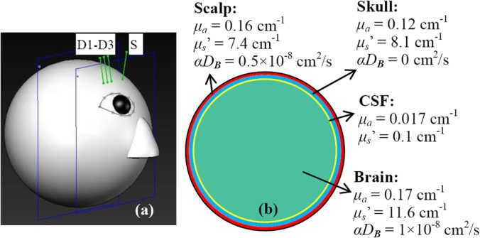
To evaluate the accuracy of the proposed Nth-order linear algorithm (Eqs. (15)–(18)) and corresponding errors (Eq. (20)), we built a simple 4-layer spherical model of adult head with multiple source and detector fibers on it for DCS data collection (Fig. 1). As shown in Fig. 1(b), the layers of head in order from outer to inner represent scalp, skull, CSF, and brain tissues, respectively.^10,11 According to multiple-scattering theory,^2,3,13 g₁(τ) decay results from the scattering events of moving scatterers, and can be quantified using Eq. (1) (for homogenous tissues) and Eq. (3) (for heterogeneous tissues). It is known from the literature¹¹ that the CSF has very low absorption and scattering coefficients (i.e., μ_a = 0.017 cm⁻¹ and μ_s′ = 0.1 cm⁻¹) compared to other layered tissues (μ_a > 0.1 cm⁻¹ and μ_s′ > 7 cm⁻¹ for scalp, skull, and brain). Therefore, the weight of CSF (depending on 1/l^*= μ_s^') contributing to g₁(τ) decay (Eq. (3)) is remarkably less than those of other layers, and thus its contribution can be ignored. However, the existing of CSF layer does influence the photon pathlengths in other tissue layers, thus affecting their BFIs (associated with g₁(τ) decay).

FIG. 1.

A sphere with 4-layer tissues (scalp, skull, CSF, and brain) to mimic an adult human head model. One source (S) and three detector (D1–D3) fibers were placed on the forehead of the model (a). S-D separations were set as 2.0, 2.5, and 3.0 cm, respectively. The scalp, skull, and CSF with the thicknesses of 0.4, 0.6, and 0.1 cm, respectively were illustrated in the cross-section view of the sphere model (b). Tissue optical properties (μ_a, μ_s', and αD_B) of the 4-layer tissues were assigned according to the literature.¹¹

The S-D separations were set as 2.0, 2.5, and 3.0 cm (Fig. 1(a)). The dimension and measurement setup matched approximately the in vivo experiments in adult brains.^7,15 The Monte Carlo simulations of 10 × 10⁶ photon migrations in heterogeneous tissues were utilized to generate w(p) and s(i, p, j) inside the head model.⁸ These values were then combined with the assigned BFIs (αD_B) and optical properties (i.e., μ_a and μ_s′)¹¹ marked in Fig. 1(b) to generate a g₁(τ) at each detector based on Eq. (3). From the generated g₁(τ) curves at multiple S-D separations, we extracted BFIs using the semi-infinite homogenous solution and Nth-order linear algorithm, respectively. Note that only the BFIs in three tissue layers (i.e., scalp, skull, brain) were extracted using the Nth-order linear algorithm because the CSF layer contributes little to the decay of g₁(τ). Similar to our previous study,⁹ DCS data with the delay times of 0.2 ≤ τ ≤ 30 μs (78 data points) were used for extracting αD_B values in the linear algorithm.

To test the capability of the N-order linear algorithm for extracting relative changes of cerebral blood flow (rCBF) in deep brain, we assigned ten levels of αD_B in the brain layer with a step decrement of 10% (i.e., αD_B (k) = [1 − (k − 1)/10] × 10⁻⁸ cm²/s, k = 1,2,…,10) while maintaining the αD_B values constant in other layers. This protocol simulates CBF changes during functional stimulations (e.g., visual and motor cortex stimuli or memory tests^7,15).

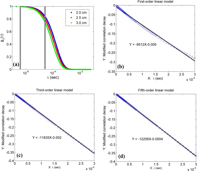
Figure 2(a) shows g₁(τ) curves generated by Eq. (3) with the assigned αD_B values at the first step (i.e., αD_B = 0.5, 0, and 1 × 10⁻⁸ cm²/s for scalp, skull, and brain, respectively). Larger S-D separations resulted in longer photon pathlength and faster decay of autocorrelation function. To examine the fitting of the linear model to the DCS data, we defined the left sides of Eqs. (15) and (17) as the modified autocorrelation decays (MADs). Figs. 2(b)–2(d) show the linear regressions of MADs at the S-D separation of 3.0 cm using the first-order (b), third-order (c), and fifth-order (d) linear models (Eqs. (15) and (17)). Higher-order (i.e., N ≥ 3) linear models exhibited excellent linear relationships between the MADs and delay time τ (Figs. 2(c) and 2(d)).

FIG. 2.

g₁(τ) curves at three S-D separations generated by Eq. (3) (a) and Nth-order liner fitting results ((b)–(d)) at the first variation step of BFIs (i.e., αD_B = 0.5, 0, and 1 × 10⁻⁸ cm²/s for scalp, skull, and brain, respectively). The 78 DCS data points (at S-D separation of 3.0 cm) with 0.2 ≤ τ ≤ 30 μs between the two grey lines (a) were used to perform the linear regressions using first-order (b), third-order (c) and fifth-order (d) linear model (Eqs. (15) and (17)).

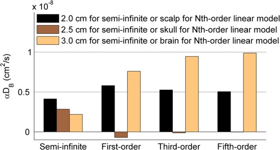
Figure 3 shows the BFIs calculated by the semi-infinite homogenous solution and the Nth-order linear algorithm (N = 1, 3, and 5) at the first step (i.e., αD_B = 0.5, 0, and 1 × 10⁻⁸ cm²/s for scalp, skull, and brain, respectively). The semi-infinite homogenous solution extracted the BFIs separately from DCS data at different S-D separations (i.e., 2.0, 2.5, or 3.0 cm). Based on photon diffusion theory in biological tissues, light penetration depth depends on tissue optical properties and the S-D separation.¹ The maximum penetration depth is approximately one half of the S-D separation. Therefore, it is not surprising that the BFI decreased with the increase of S-D separation (Fig. 3) since photons detected at larger separations travel inside the skull layer (αD_B = 0) more than other layers (αD_B > 0). By contrast, the linear algorithm (Eqs. (15)–(18)) used DCS data at all S-D separations simultaneously to extract BFIs at different layer tissues. The estimation errors of BFIs decreased with the increase of the order number. Using the fifth-order solution, for example, the reconstructed errors of αD_B in different tissue layers were less than 3%, and fell into the range estimated by Eq. (20). In fact, the linear model with higher orders (N > 5) generated even smaller errors (<2%) in calculating BFIs in different layers (data are not shown).

FIG. 3.

The BFIs (i.e., αD_B) calculated by the semi-infinite homogeneous solution at three S-D separations (i.e., 2.0, 2.5, or 3.0 cm) and the Nth-order linear algorithm (N = 1, 3, and 5) at the first variation step of BFIs (i.e., αD_B = 0.5, 0, and 1 × 10⁻⁸ cm²/s for scalp, skull, and brain, respectively). The reconstructed errors of αD_B decreased with the increase of the order number, and the solutions with higher orders (i.e., N ≥ 3) generated smaller αD_B errors than the semi-infinite solution.

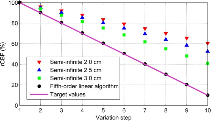
To compare the accuracies of the semi-infinite homogenous solution and the high-order linear algorithm for quantifying rCBF in deep brain, BFIs at the ten variation steps were calculated using both methods. All BFIs were normalized (divided) to their reconstructed values at the first variation step, respectively, and presented as percentage changes (%). As shown in Fig. 4, rCBF values extracted by the fifth-order linear algorithm were highly consistent with the assigned true flow values at all steps (errors < 3%). By contrast, the semi-infinite homogenous solution resulted in large errors in rCBF over the ten steps (34.5% ≤ errors ≤ 60.2%). As expected, the estimation errors increased with the decrease of S-D separation.

FIG. 4.

rCBF (%) calculated by the semi-infinite solution at three S-D separations and the fifth-order linear model at the 10 variation steps of BFIs. CBF values were normalized to their reconstructed values at the first variation step and presented as rCBF (%). The fifth-order linear algorithm extracted much more accurate rCBF values over the 10 variation steps compared to the semi-infinite homogenous solution.

In summary, we have extended our previous Nth-order linear algorithm for extracting BFI and rBF in homogenous tissues⁹ to heterogeneous tissues. This algorithm integrates a Nth-order linear model and Monte Carlo simulation of photon migrations in heterogeneous tissues with arbitrary geometry, and utilizes the DCS data at multiple S-D separations simultaneously. As long as the one-time Monte Carlo simulation is done, the linear model requires only simple algebraic calculations (Eqs. (17) and (18)), thus allowing for online data processing and displaying. Simulation results on an adult head model with 4-layer tissues of scalp, skull, CSF, and brain demonstrate its accuracy in extracting both BFI and rBF values in different layers. Although we have tested this linear algorithm only on the simple spherical layer tissues, arbitrary tissue geometry and volume can be obtained and tested in the future by incorporating other imaging modalities (e.g., MRI). By contrast, the semi-infinite homogenous solution is susceptible to overlaying tissues, leading to substantial evaluation errors in BFIs of layered tissues and underestimations in rCBF (i.e., partial volume effect¹⁴).

Note that for simplicity, we assumed scalp blood flow remains constant in the simulation, which may not be true during specific physiological manipulations (e.g., head-up bed titling, breath-holding).¹⁶ Future study will test this linear algorithm for the use in heterogeneous tissues with different levels of blood flow variations and noises.

References

- 1.Durduran T. and Yodh A. G., Neuroimage 85, 51 (2014). 10.1016/j.neuroimage.2013.06.017 [DOI] [PMC free article] [PubMed] [Google Scholar]
- 2.Pine D. J., Weitz D. A., Chaikin P. M., and Herbolzheimer E., Phys. Rev. Lett. 60(12), 1134 (1988). 10.1103/PhysRevLett.60.1134 [DOI] [PubMed] [Google Scholar]
- 3.Maret G. and Wolf P. E., Z. Phys. B: Condens. Matter 65(4), 409 (1987). 10.1007/BF01303762 [DOI] [Google Scholar]
- 4.Cheung C., Culver J. P., Takahashi K., Greenberg J. H., and Yodh A. G., Phys. Med. Biol. 46(8), 2053 (2001). 10.1088/0031-9155/46/8/302 [DOI] [PubMed] [Google Scholar]
- 5.Roche-Labarbe N., Carp S. A., Surova A., Patel M., Boas D. A., Grant R. E., and Franceschini M. A., Hum. Brain Mapp. 31(3), 341 (2010). 10.1002/hbm.20868 [DOI] [PMC free article] [PubMed] [Google Scholar]
- 6.Dong J., Bi R. Z., Ho J. H., Thong P. S. P., Soo K. C., and Lee K., J. Biomed. Opt. 17(9), 097004 (2012). 10.1117/1.JBO.17.9.097004 [DOI] [PubMed] [Google Scholar]
- 7.Jaillon F., Li J., Dietsche G., Elbert T., and Gisler T., Opt. Express 15(11), 6643 (2007). 10.1364/OE.15.006643 [DOI] [PubMed] [Google Scholar]
- 8.Li T., Lin Y., Shang Y., He L., Huang C., Szabunio M., and Yu G., Sci. Rep. 3, 1358 (2013). 10.1038/srep01358 [DOI] [PMC free article] [PubMed] [Google Scholar]
- 9.Shang Y., Li T., Chen L., Lin Y., Toborek M., and Yu G., Appl. Phys. Lett. 104(19), 193703 (2014). 10.1063/1.4876216 [DOI] [PMC free article] [PubMed] [Google Scholar]
- 10.Jaillon F., Skipetrov S. E., Li J., Dietsche G., Maret G., and Gisler T., Opt. Express 14(22), 10181 (2006). 10.1364/OE.14.010181 [DOI] [PubMed] [Google Scholar]
- 11.Gagnon L., Desjardins M., Jehanne-Lacasse J., Bherer L., and Lesage F., Opt. Express 16(20), 15514 (2008). 10.1364/OE.16.015514 [DOI] [PubMed] [Google Scholar]
- 12.Shang Y., Chen L., Toborek M., and Yu G., Opt. Express 19(21), 20301 (2011). 10.1364/OE.19.020301 [DOI] [PMC free article] [PubMed] [Google Scholar]
- 13.Boas D. A. and Yodh A. G., J. Opt. Soc. Am. A 14(1), 192 (1997). 10.1364/JOSAA.14.000192 [DOI] [PubMed] [Google Scholar]
- 14.Durduran T., Choe R., Baker W. B., and Yodh A. G., Rep. Prog. Phys. 73(7), 076701 (2010). 10.1088/0034-4885/73/7/076701 [DOI] [PMC free article] [PubMed] [Google Scholar]
- 15.Li J., Dietsche G., Iftime D., Skipetrov S. E., Maret G., Elbert T., Rockstroh B., and Gisler T., J. Biomed. Opt. 10(4), 44002 (2005). 10.1117/1.2007987 [DOI] [PubMed] [Google Scholar]
- 16.Cheng R., Shang Y., Hayes D., Saha S. P., and Yu G., Neuroimage 62(3), 1445 (2012). 10.1016/j.neuroimage.2012.05.069 [DOI] [PubMed] [Google Scholar]