Suppressing qubit dephasing using real-time Hamiltonian estimation

Abstract

Unwanted interaction between a quantum system and its fluctuating environment leads to decoherence and is the primary obstacle to establishing a scalable quantum information processing architecture. Strategies such as environmental and materials engineering, quantum error correction and dynamical decoupling can mitigate decoherence, but generally increase experimental complexity. Here we improve coherence in a qubit using real-time Hamiltonian parameter estimation. Using a rapidly converging Bayesian approach, we precisely measure the splitting in a singlet-triplet spin qubit faster than the surrounding nuclear bath fluctuates. We continuously adjust qubit control parameters based on this information, thereby improving the inhomogenously broadened coherence time from tens of nanoseconds to >2 μs. Because the technique demonstrated here is compatible with arbitrary qubit operations, it is a natural complement to quantum error correction and can be used to improve the performance of a wide variety of qubits in both meteorological and quantum information processing applications.

Decoherence is anathema to quantum systems, as it reduces their performance and stability. Shulman et al. show that real-time Hamiltonian parameter estimation can significantly increase the coherence time of a qubit by enabling continuous adjustment of its control parameters.

Hamiltonian parameter estimation is a rich field of active experimental and theoretical research that enables precise characterization and control of quantum systems1. For example, magnetometry schemes employing Hamiltonian learning have demonstrated dynamic range and sensitivities exceeding those of standard methods2,3. Such applications focused on estimating parameters that are quasistatic on experimental timescales. However, the effectiveness of Hamiltonian learning also offers exciting prospects for estimating fluctuating parameters responsible for decoherence in quantum systems.

The quantum system that we study is a singlet-triplet (S−T₀) qubit4,5 which is formed by two gate-defined lateral quantum dots (QDs) in a GaAs/AlGaAs heterostructure (Fig. 1a, Supplementary Fig. 1), similar to that of refs 6, 7. The qubit can be rapidly initialized in the singlet state |S› in ≈20 ns and read out with 98% fidelity in ≈1 μs (refs 8, 9; Supplementary Fig. 2). Universal quantum control is provided by two distinct drives10: the exchange splitting, J, between |S› and |T₀›, and the magnetic field gradient, ΔB_z, due to the hyperfine interaction with host Ga and As nuclei. The Bloch sphere representation for this qubit can be seen in Fig. 1b. In this work, we focus on qubit evolution around ΔB_z (Fig. 2a). Due to statistical fluctuations of the nuclei, ΔB_z varies randomly in time, and consequently oscillations around this field gradient decay in a time (ref. 4). A nuclear feedback scheme relying on dynamic nuclear polarization11 can be employed to set the mean gradient, (g*μ_BΔB_z/h≈60 MHz in this work) as well as reduce the variance of the fluctuations. Here, g*≈−0.44 is the effective gyromagnetic ratio in GaAs, μ_B is the Bohr magneton and h is Planck’s constant. In what follows, we adopt units where g*μ_B/h=1. The nuclear feedback relies on the avoided crossing between the |S› and |T₊› states. When the electrons are brought adiabatically through this crossing, their total spin changes by Δm_s=±1, which is accompanied by a nuclear spin flip to conserve angular momentum. With the use of this feedback, the coherence time improves to (ref. 11; Fig. 2b), limited by the low nuclear pumping efficiency10. Crucially, the residual fluctuations are considerably slower than the timescale of qubit operations12.

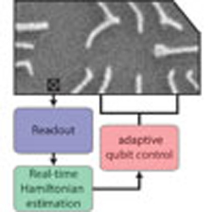
Figure 1. Experimental apparatus.

(a) A scanning electron microscope image of the double QD with a schematic of the apparatus used for adaptive qubit control. A floating metal gate protruding from the right can be seen which increases the capacitance between the qubit and an adjacent qubit (not pictured), which is left inactive for this work. The reflected read-out drive signal is demodulated to DC, digitized by a correlated double sampler (CDS), and ΔB_z is estimated in real time by the field-programmable gate array (FPGA). The FPGA updates the digital to analogue converter (DAC) to keep the voltage controlled oscillator (VCO) resonant with the estimated value of ΔB_z. The VCO controls the voltage detuning, ε(t) between the QDs, which, in turn, modulates J at Ω_J. (b) The Bloch sphere representation for the S−T₀ qubit showing the two axes of control, J and ΔB_z.

Figure 2. ΔB_z oscillations.

(a) The pulse sequence used to estimate ΔB_z. (b) Using nuclear feedback, ΔB_z oscillations decay in a coherence time due to residual slow fluctuations in ΔB_z. (c) The Ramsey sequence used to operate the S-T₀ qubit in the rotating frame. (d) The Ramsey contrast (blue dots) decays in a characteristic time (solid line fit ) similar to the oscillations in b due to the same residual slow fluctuations in ΔB_z. (e) The Rabi pulse sequence used to drive the qubit in the rotating frame. (f) The rotating frame S−T₀ qubit exhibits the typical behaviour when sweeping drive frequency and time (top). When driven on resonance (bottom), the qubit undergoes Rabi oscillations, demonstrating control in the rotating frame.

In this work we employ techniques from Hamiltonian estimation to prolong the coherence of a qubit by more than a factor of 30. Importantly, our estimation protocol, which is based on recent theoretical work13, requires relatively few measurements (≈100) which we perform rapidly enough (total time ≈100 μs) to resolve the qubit splitting faster than its characteristic fluctuation time. We adopt a paradigm in which we separate experiments into ‘estimation’ and ‘operation’ segments, and we use information from the former to optimize control parameters for the latter in real-time. Our method dramatically prolongs coherence without using complex pulse sequences such as those required for non-identity dynamically decoupled operations14.

Results

Rotating frame S−T ₀ qubit

To take advantage of the slow nuclear dynamics, we introduce a method that measures the fluctuations and manipulates the qubit on the basis of precise knowledge but not precise control of the environment. We operate the qubit in the rotating frame of ΔB_z, where qubit rotations are driven by modulating J at the frequency (refs 15, 16). This is in contrast to traditional modes of operation of the S−T₀ qubit, which rely on DC voltage pulses. To measure Rabi oscillations, the qubit is adiabatically prepared in the ground state of ΔB_z (|ψ›=|↑↓›), and an oscillating J is switched on (Fig. 2e), causing the qubit to precess around J in the rotating frame. In addition, we perform a Ramsey experiment (Fig. 2c) to determine , and as expected, we observe the same decay (Fig. 2d) as Fig. 2b. More precisely, the data in Fig. 2d represent the average of 1,024 experimental repetitions of the same qubit operation sequence immediately following nuclear feedback. The feedback cycle resets ΔB_z to its mean value (60 MHz) with residual fluctuations of between experimental repetitions. However, within a given experimental repetition, ΔB_z is approximately constant. Therefore we present an adaptive control scheme where, following nuclear feedback, we quickly estimate ΔB_z and tune to prolong qubit coherence (Fig. 3a).

Figure 3. Adaptive control.

(a) For these measurements we first perform our standard nuclear feedback, then quickly estimate ΔB_z and update the qubit control, then operate the qubit at the correct driving frequency. (b) Using adaptive control, we perform a Ramsey experiment (deliberately detuned to see oscillations) and obtain coherence times of . (c) Histograms of measured Ramsey detunings with (green) and without (blue) adaptive control. For clarity, these data were taken with a different mean detuning than those in b. (d) Raw data for 1,024 consecutive Ramsey experiments with adaptive control lasting 250 s in total. A value of 1 corresponds to |T₀› and 0 corresponds to |S›. Stabilized oscillations are clearly visible in the data, demonstrating the effect of adaptive control.

Bayesian estimation

To estimate ΔB_z , we repeatedly perform a series of single-shot measurements after allowing the qubit to evolve around ΔB_z (using DC pulses) for some amount of time (Fig. 2a). Rather than fixing this evolution time to be constant for all trials, we make use of recent theoretical results in Hamiltonian parameter estimation13,16,17 and choose linearly increasing evolution times, t_k=kt_samp, where k=1,2,…N. We choose the sampling time t_samp such that the estimation bandwidth is several times larger than the magnitude of the residual fluctuations in ΔB_z, roughly 10 MHz. With a Bayesian approach to estimate ΔB_z in real-time, the longer evolution times (large k) leverage the increased precision obtained from earlier measurements to provide improved sensitivity, allowing the estimate to outperform the standard limit associated with repeating measurements at a single evolution time. Denoting the outcome of the kth measurement as m_k (either |S› or |T₀›), we define P(m_k|ΔB_z) as the conditional probability for m_k given a value ΔB_z. We write

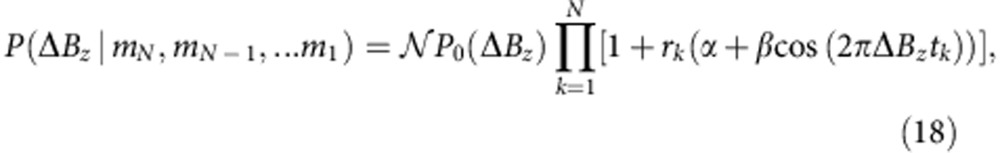
where r_k=1 (−1) for m_k=|S›(|T₀›), and α=0.25 and β=0.67 are parameters determined by the measurement error and axis of rotation on the Bloch sphere (see Methods). Since we assume that earlier measurement outcomes do not affect later ones (that is, that there is no measurement back-action), we write the conditional probability for ΔB_z given the results of N measurements as:

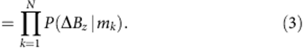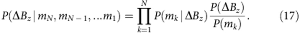
Using Bayes’ rule, that is, P(ΔB_z|m_k)=P(m_k|ΔB_z)P(ΔB_z)/P(m_k), and equation (1), we can rewrite equation (3) as:

where N is a normalization constant and P₀(ΔB_z) is a prior distribution to which the algorithm is empirically insensitive, and which we take to be a constant over the estimation bandwidth. After the last measurement, we find the value of ΔB_z that maximizes the posterior distribution P(ΔB_z|m_N,m_N−1,...m₁).

Adaptive control

We implement this algorithm in real-time on a field-programmable gate array (FPGA), computing P(ΔB_z) for 256 values of ΔB_z between 50 and 70 MHz. With each measurement m_k, the read-out signal is digitized and passed to the FPGA, which computes P(ΔB_z) and updates an analogue voltage that tunes the frequency of a voltage controlled oscillator (Fig. 1a; Supplementary Note 1, Supplementary Fig. 3). Following the Nth sample, nearly matches ΔB_z, and since the nuclear dynamics are slow, the qubit can be operated with long coherence without any additional complexity. To quantify how well the FPGA estimate matches ΔB_z, we perform a Ramsey experiment (deliberately detuned to observe oscillations) with this real-time tracking of ΔB_z and find optimal performance for N≈120, with a maximum experimental repetition rate, limited by the FPGA, of 250 kHz and a sampling time t_samp=12 ns. Under these conditions, and making a new estimate after every 42 Ramsey experiments, we observe , a 30-fold increase in coherence (Fig. 3b). We note that these data are taken with the same pulse sequence as those in Fig. 2d. To further compare qubit operations with and without this technique, we measure Ramsey fringes for ≈250 s (Fig. 3d), and histogram the observed Ramsey detunings. With adaptive control we observe a stark narrowing of the observed frequency distribution, consistent with this improved coherence (Fig. 3c).

Discussion

Although the estimation scheme employed here is theoretically predicted to improve monotonically with N (ref. 13), we find that there is an optimum (N≈120), after which slowly decreases with increasing N (Fig. 4a). A possible explanation for this trend is fluctuation of the nuclear gradient during the estimation period. To investigate this, we obtain time records of ΔB_z using the Bayesian estimate and find that its variance increases linearly in time at the rate of (6.7±0.7 kHz)² μs⁻¹ (Fig. 4c). The observed linear behaviour suggests a model where the nuclear gradient diffuses, which can arise, for example, from dipolar coupling between adjacent nuclei. Using the measured diffusion of ΔB_z, we simulate the performance of the Bayesian estimate as a function of N (see Methods). Given that the simulation has no free parameters, we find good agreement with the observed , indicating that indeed, diffusion limits the accuracy with which we can measure ΔB_z (Fig. 4a).

Figure 4. ΔB_z diffusion.

(a) The coherence time, using the adaptive control and for a simulation show a peak, indicating that there is an optimal number of measurements to make when estimating ΔB_z. (b) When many time traces of ΔB_z are considered, their variance grows linearly with time, indicating a diffusion process. (c) The scaling of as a function of T_delay for software scaled data is consistent with diffusion of ΔB_z. The red line is a fit to a diffusion model. (d) The performance of the Bayesian estimate of ΔB_z can be estimated using software post-processing, giving , which corresponds to a precision of .

This model suggests that increasing the rate of measurements during estimation will improve the accuracy of the Bayesian estimate. Because our FPGA limits the repetition rate of qubit operations to 250 kHz, we demonstrate the effect of faster measurements through software post-processing with the same Bayesian estimate. To do so, we first use the same estimation sequence, but for the operation segment, we measure the outcome after evolving around ΔB_z for a single evolution time, t_evo, rather than performing a rotating frame Ramsey experiment, and we repeat this experiment a total of N_tot times. In processing, we perform the Bayesian estimate of each ΔB_z,i, sort the data by adjusted time (for i=1,2,…N_tot), and average together points of similar τ to observe oscillations (see Methods). We fit the decay of these oscillations to extract and the precision of the Bayesian estimate, . For the same operation and estimation parameters, we find that extracted from software post-processing agrees with that extracted from adaptive control Supplementary Fig. 4, Supplementary Note 2. Using a repetition rate as high as 667 kHz, we show coherence times above 2,800 ns, corresponding to an error of σ_ΔBz=80 kHz (Fig. 4d), indicating that improvements are easily attainable by using faster (commercially available) FPGAs.

In addition, we use this post-processing to examine the effect of this technique on the duty cycle of experiments as well as the stability of the ΔB_z estimate. To do so we introduce a delay T_delay between the estimation of ΔB_z and the single evolution measurement performed in place of the operation. We find , where c=0.99 (Fig. 4c), consistent with diffusion of ΔB_z. Indeed, this dependence underscores the potential of adaptive control, since it demonstrates that after a single estimation sequence, the qubit can be operated for >1 ms with . Thus, adaptive control need not significantly reduce the experimental duty cycle.

In this work, we have used real-time adaptive control on the basis of Hamiltonian parameter estimation of a S−T₀ spin qubit to prolong from 70 ns to >2 μs. Dephasing due to nuclear spins has long been considered a significant obstacle to quantum information processing using semiconductor spin qubits18, and elimination of nuclear spins is an active and fruitful area of research19,20,21. However, here we have shown that with a combination of nuclear feedback, rotating frame S−T₀ spin resonance, and real-time Hamiltonian estimation, we are able to achieve ratios of coherence times to operation times in excess of 200 without recourse to dynamical decoupling12,22,23. If the same adaptive control techniques were applied to gradients as high as 1 GHz (ref. 10), ratios exceeding 4,000 would be possible, and longer coherence times may be attainable with more sophisticated techniques13. Though the observed coherence times are still smaller than the Hahn echo time, (ref. 12), the method we have presented is straightforward to implement, compatible with arbitrary qubit operations, and general to all qubits that suffer from non-Markovian noise. Looking ahead, it is likely, therefore, to have a key role in realistic quantum error correction efforts24,25,26,27, where even modest improvements in baseline error rate greatly diminish experimental complexity and enhance prospects for a scalable quantum information processing architecture.

Methods

Bayesian estimate

We wish to calculate the probability that the nuclear magnetic field gradient has a certain value, ΔB_z, given a particular measurement record comprising N measurements. We follow the technique in Sergeevich et al.13 with slight modifications. Writing the outcome of the kth measurement as m_k, we write this probability distribution as

To arrive at an expression for this distribution, we will write down a model for the dynamics of the system, that is, P(m_N,m_N−1,...m₁|ΔB_z). Using Bayes’ rule we can relate the two equations as

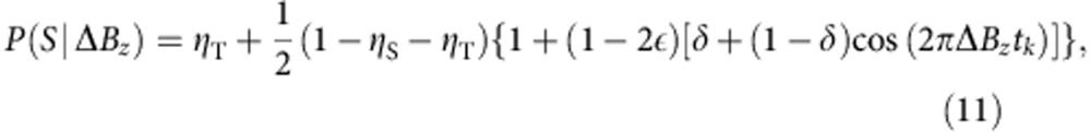
First, we seek a model that can quantify P(m_N,m_N−1,...m₁|ΔB_z) that accounts for realistic errors in the system, namely measurement error, imperfect state preparation and error in the axis of rotation around the Bloch sphere. For simplicity, we begin with a model that accounts only for measurement error. Denoting the error associated with measuring a |S› (|T₀›) as η_S (η_T), we write

We combine these two equations and write

where r_k=1 (−1) for m_k=|S›(|T₀›) and α and β are given by

Next, we generalize the model to include the effects of imperfect state preparation, and the presence of non-zero J during evolution, which renders the initial state non-orthogonal to the axis of rotation around the Bloch sphere (see above). We assume that the angle of rotation around the Bloch sphere lies somewhere in the x–z plane and makes an angle θ with the z axis. We define δ=cos² (θ). Next, we include imperfect state preparation by writing the density matrix ρ_init=(1−ε)|S› ‹S|)+ε|T₀› ‹T₀|. With this in hand, we can write down the model

Using the same notation for r_k=1 (−1) for m_k=|S›(|T₀›), we rewrite this in one equation as

where we now have

We find the best performance for α=0.25 and β=0.67, which is consistent with known values for qubit errors.

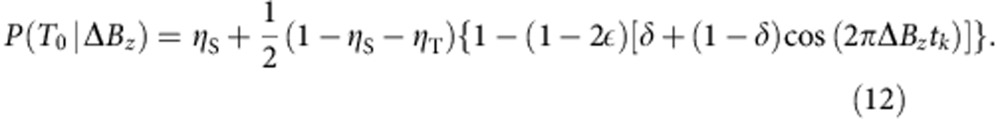
We next turn our attention to implementing Bayes’ rule to turn this model into a probability distribution for ΔB_z. First, we assume that all measurements are statistically independent, allowing us to write

We next use Bayes rule (6) and rewrite this equation as

Using our model (13) we can rewrite this as

where N is a normalization constant, and P₀(ΔB_z) is a prior distribution for ΔB_z which we take to be a constant over the estimation bandwidth, and to which the estimator is empirically insensitive. With this formula, it is simple to see that the posterior distribution for ΔB_z can be updated in real time with each successive measurement. After the Nth measurement, we choose the value for ΔB_z, which maximizes the posterior distribution (18).

Simulation with diffusion

We simulate the performance of our software scaling and hardware (FPGA) estimates of ΔB_z using the measured value of the diffusion rate. We assume that ΔB_z obeys a random walk, but assume that during a single evolution time t_k, ΔB_z is static. This assumption is valid when 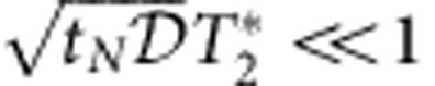, where is the diffusion rate of ΔB_z. For an estimation of ΔB_z with N different measurements, we generate a random walk of N different values for ΔB_z (using the measured diffusion), simulate the outcome of each measurement, and compute the Bayesian estimate of ΔB_z using the simulated outcomes. By repeating this procedure 4,096 times, and using the mean squared error, MSE=‹(ΔB_z−ΔB_z^estimated)²› as a metric for performance, we can find the optimal number of measurements to perform. To include the entire error budget of the FPGA apparatus, we add to this MSE the error from the phase noise of the VCO, the measured voltage noise on the analogue output controlling the VCO, and the diffusion of ΔB_z during the ‘operation’ period of the experiment.

Software post-processing

The estimate of ΔB_z can be independently verified using software analysis. In this experiment, we use the same method to estimate ΔB_z as in the adaptive control experiment, but in the operation segment perform oscillations around ΔB_z for verification. We choose m different evolution times and measure each n times for a total of N_tot=m × n measurements of ΔB_z. In the ith experiment (i=1,2,…N_tot), we evolve for a time t_evo,i, accumulating phase φ_i=ΔB_z,it_evo,i. Because we make a precise measurement of ΔB_z at the start of each experiment, we can employ it to rescale the time, t_evo,i, so that the phase accumulated for a given time is constant using the equation,

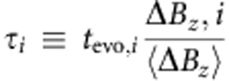This sets φ_i(τ_i)=‹ΔB_z›τ_i, with residual error arising from inaccuracy in the estimate of ΔB_z,i. The data are then sorted by τ, and points of similar τ are averaged using a Gaussian window with σ_τ=0.5 ns≪T≈16 ns, where T is the period of the oscillations.

Author contributions

V.U. prepared the crystal M.D.S. fabricated the sample, J.M.N. programmed the FPGA, M.D.S, S.P.H., J.M.N., S.D.B, A.C.D, and A.Y. carried out the experiment, analyzed the data, and wrote the paper.

Additional information

How to cite this article: Shulman, M. D. et al. Suppressing qubit dephasing using real-time Hamiltonian estimation. Nat. Commun. 5:5156 doi: 10.1038/ncomms6156 (2014).

Supplementary Material

Supplementary Information

Supplementary Figures 1-4 and Supplementary Notes 1-2

References

- Wiseman Howard M. & Milburn Gerard J. Quantum Measurement and Control Cambridge Univ. Press (2010). [Google Scholar]
- Waldherr G. et al. High-dynamic-range magnetometry with a single nuclear spin in diamond. Nat. Nanotechnol. 7, 105–108 (2012). [DOI] [PubMed] [Google Scholar]
- Nusran N. M., Ummal M. & Gurudev Dutt M. V. High dynamic range magnetometry with a single electronic spin in diamond. Nat. Nanotechnol. 7, 109–113 (2012). [DOI] [PubMed] [Google Scholar]
- Petta J. R. et al. Coherent manipulation of coupled electron spins in semiconductor quantum dots. Science 309, 2180–2184 (2005). [DOI] [PubMed] [Google Scholar]
- Maune B. M. et al. Coherent singlet-triplet oscillations in a silicon-based double quantum dot. Nature 481, 344–347 (2011). [DOI] [PubMed] [Google Scholar]
- Dial O. E. et al. Charge noise spectroscopy using coherent exchange oscillations in a singlet-triplet qubit. Phys. Rev. Lett. 110, 146804 (2013). [DOI] [PubMed] [Google Scholar]
- Shulman M. D. et al. Demonstration of entanglement of electrostatically coupled singlet-triplet qubits. Science 336, 202–205 (2012). [DOI] [PubMed] [Google Scholar]
- Barthel C., Reilly D. J., Marcus C. M., Hanson M. P. & Gossard. A. C. Rapid single-shot measurement of a singlet-triplet qubit. Phys. Rev. Lett. 103, 160503 (2009). [DOI] [PubMed] [Google Scholar]
- Reilly D. J., Marcus C. M., Hanson M. P. & Gossard A. C. Fast single-charge sensing with a RF quantum point contact. Appl. Phys. Lett. 91, 162101 (2007). [Google Scholar]
- Foletti S., Bluhm H., Mahalu D., Umansky V. & Yacoby A. Universal quantum control in two-electron spin quantum bits using dynamic nuclear polarization. Nat. Phys. 5, 903–908 (2009). [Google Scholar]
- Bluhm H., Foletti S., Mahalu D., Umansky V. & Yacoby A. Enhancing the coherence of a spin qubit by operating it as a feedback loop that controls its nuclear spin bath. Phys. Rev. Lett. 105, 216803 (2010). [DOI] [PubMed] [Google Scholar]
- Bluhm H. et al. Dephasing time of GaAs electron-spin qubits coupled to a nuclear bath exceeding 200 μs. Nat. Phys. 7, 109–113 (2011). [Google Scholar]
- Sergeevich A., Chandran A., Combes J., Bartlett S. D. & Wiseman H. M. Characterization of a qubit Hamiltonian using adaptive measurements in a fixed basis. Phys. Rev. A 84, 052315 (2011). [Google Scholar]
- Kestner J. P., Wang X., Bishop L. S., Barnes E. & Das Sarma S. Noise-resistant control for a spin qubit array. Phys. Rev. Lett. 110, 140502 (2013). [DOI] [PubMed] [Google Scholar]
- Coish W. A. & Loss D. Hyperfine interaction in a quantum dot: non-Markovian electron spin dynamics. Phys. Rev. B 70, 195340 (2004). [Google Scholar]
- Klauser D., Coish W. A. & Loss D. Nuclear spin state narrowing via gate-controlled Rabi oscillations in a double quantum dot. Phys. Rev. B 73, 205302 (2006). [Google Scholar]
- Ferrie C., Granade C. E. & Cory D. G. How to best sample a periodic probability distribution, or on the accuracy of Hamiltonian finding strategies. Quantum Inf. Process. 12, 611 (2013). [Google Scholar]
- Schroer M. D. & Petta J. R. Quantum dots: time to get the nukes out. Nat. Phys. 4, 516–518 (2008). [Google Scholar]
- Balasubramanian G. et al. Ultralong spin coherence time in isotopically engineered diamond. Nat. Mater. 8, 383–387 (2009). [DOI] [PubMed] [Google Scholar]
- Wild A. et al. Few electron double quantum dot in an isotopically purified 28Si quantum wel. Appl. Phys. Lett. 100, 143110 (2012). [Google Scholar]
- Muhonen J. T. et al. Storing quantum information for 30 seconds in a nanoelectronic device. Preprint at http://arxiv.org/abs/1402.7140 (2014). [DOI] [PubMed]
- Hahn E. L. Spin echoes. Phys. Rev. 80, 580–594 (1950). [Google Scholar]
- Uhrig G. S. Exact results on dynamical decoupling by pi pulses in quantum inforamtion processes. New J. Phys. 10, 083024 (2008). [Google Scholar]
- Nielsen M. A. & Chuang I. L. Quantum Computation and Quantum Information Cambridge Univ. Press (2000). [Google Scholar]
- Reed M. D. et al. Realization of a three-qubit quantum error correction with superconducting circuits. Nature 482, 382–385 (2011). [DOI] [PubMed] [Google Scholar]
- Waldherr G. et al. Quantum error correction in a solid-state hybrid spin register. Nature 506, 204–207 (2014). [DOI] [PubMed] [Google Scholar]
- Taminiau T. H., Cramer J., Van der Sar T., Dobrovitski V. V. & Hanson R. Universal control and error correction in multi-qubit spin registers in diamond. Nat. Nanotechnol. 9, 171–176 (2014). [DOI] [PubMed] [Google Scholar]
Associated Data
This section collects any data citations, data availability statements, or supplementary materials included in this article.
Supplementary Materials