Statistical normalization techniques for magnetic resonance imaging

Abstract

While computed tomography and other imaging techniques are measured in absolute units with physical meaning, magnetic resonance images are expressed in arbitrary units that are difficult to interpret and differ between study visits and subjects. Much work in the image processing literature on intensity normalization has focused on histogram matching and other histogram mapping techniques, with little emphasis on normalizing images to have biologically interpretable units. Furthermore, there are no formalized principles or goals for the crucial comparability of image intensities within and across subjects. To address this, we propose a set of criteria necessary for the normalization of images. We further propose simple and robust biologically motivated normalization techniques for multisequence brain imaging that have the same interpretation across acquisitions and satisfy the proposed criteria. We compare the performance of different normalization methods in thousands of images of patients with Alzheimer's disease, hundreds of patients with multiple sclerosis, and hundreds of healthy subjects obtained in several different studies at dozens of imaging centers.

Highlights

• •Formalize the necessity and goals of statistical intensity normalization
• •Novel approach for intensity normalization of brain MRI without prior segmentation
• •Extend the novel approach for multimodality imaging
• •Propose new quantitative metric for intensity normalization in a population
• •Evaluate normalization techniques in large multicenter studies

1. Introduction

Complex multi-modality, cross-sectional and longitudinal imaging studies are now commonplace in medical research and clinical practice. Such studies produce terabytes of highly complex data, cost millions of dollars, and require years to decades of follow-up. Many such studies have already been conducted and are currently underway to investigate a diverse collection of disabling and fatal diseases. Most of these studies include multisequence magnetic resonance imaging (MRI) to assess structural differences and changes in the brain. The nature of conventional MRI units makes direct quantitative analysis difficult; in particular, MRI scans are acquired in arbitrary units that are not comparable between study visits within a single subject nor across different subjects.

The image analysis literature has emphasized the importance of intensity normalization (which we refer to as normalization for brevity) for registration (Hellier, 2003), cross-sectional (Wang et al., 1998; Shah et al., 2011) and longitudinal (Sweeney et al., 2013a) segmentation, longitudinal quantification (Meier and Guttmann, 2003), and other measures (Madabhushi et al., 2006; Loizou et al., 2009). Much work over the past two decades has aimed to address this issue with limited success (Nyul and Udupa, 1999; Nyul et al., 2000; Weisenfeld and Warfield, 2004; Jäger et al., 2006; Madabhushi and Udupa, 2006; Leung et al., 2010) (for a comprehensive review of these methods, see Shah et al., 2011). However, as the goals of normalization have not been formalized, the comparison of these methodologies is difficult. As intensity normalization is often also a preprocessing step for later analyses, in each such case these analytical goals are most relevant. Furthermore, all previously proposed methods suffer from the lack of biological interpretability of the normalized units.

Our goal is to propose an explicit statistical framework for image intensity normalization, develop a new class of robust intensity normalization methods for studying the brain through MRI, and deploy them on thousands of images from the Australian Imaging, Biomarkers and Lifestyle Flagship Study of Aging (AIBL), the Alzheimer's Disease Neuroimaging Initiative (ADNI), and two large studies of multiple sclerosis (MS) acquired using a variety of scanners and protocols. In the next section, we describe a set of criteria that formalize the goals of normalization. We then describe a novel statistical normalization methodology and the results from this simple technique, and we conclude with a discussion.

2. Materials and methods

2.1. Principles of image normalization

Consider the image intensity Y_ij(v) at each voxel v expressed in arbitrary units and measured for subject i at visit j using a particular modality. Normalization is any transformation of the type Y_ij(v) → N_ij{Y_ij(v)}. It is useful to conceptualize the histogram of intensities Y_ij(v) as a mixture of densities:

$$f_{\mathit{ij}}\left(x\right)={\displaystyle \sum _{k=1}^K}{w}_{\mathit{ijk}}{f}_{\mathit{ijk}}\left(x\right),$$ (1)

where f_ijk(x) is the subject/visit-specific intensity densities of empty space and known tissues, such as white matter, gray matter, cerebrospinal fluid, bone, skin, and lesions. The weights w_ijk ≥ 0 sum to 1 and represent the relative weights of components k = 1, …, K. This includes both cases with and without pathology, as the weight for lesions or other abnormal tissues can be zero. Note that the densities f_ijk(x) and weights w_ijk are not directly observed, but may be estimated by first segmenting the images and estimating w_ijk using the proportion of the image in the k-th tissue class and f_ijk(x) by the histogram of intensities in that tissue.

The quantitative analysis of images assumes the existence of a theoretical model in normalized space for all images: g_ij(x) = ∑ _k = 1^K w_ijkg_k(x), where the densities g_k(x) are independent of subjects and/or visits, though the weights assigned to these densities depend on subject and visit and may be the measure of interest in studies. The fundamental difficulty of normalization is to find a transformation from f_ij(x) to g_ij(x) that respects the ordering of distributions and their mutual distances in the normalized space, and thus we denote a normalized density by ${\displaystyle {\widehat{g}}_{\mathit{ij}}}\left(x\right)$ for clarity.

Although the fundamental importance of intensity normalization has been emphasized by numerous publications in the imaging literature (Shah et al., 2011; Nyul and Udupa, 1999; Weisenfeld and Warfield, 2004), no formal guiding principles nor definitions have been established. We introduce a set of 7 principles, which we refer to as the statistical principles of image normalization (SPIN).

The normalization process should produce units that:

• 1.have a common interpretation across locations within the same tissue type
• 2.are replicable
• 3.preserve the rank of intensities
• 4.have similar distributions for the same tissues of interest within and across patients
• 5.are not influenced by biological abnormality or population heterogeneity
• 6.are minimally sensitive to noise and artifacts and
• 7.do not result in loss of information associated with pathology or other phenomena.

SPIN is motivated by the goal of population-level analysis that respects the structure of images while requiring the comparability of replicable and biologically meaningful units within tissue types within and across subjects. The preservation of ranks avoids situations where normalized image comparisons are discordant with comparisons made using raw units within a subject, and the requirements of minimal sensitivity to noise, population heterogeneity, and pathology aim to avoid spurious findings.

In the absence of SPIN, much of the work on normalization has progressed with little objective quantification or validation. To assess SPIN, several metrics may be appropriate: SPIN 1 depends on the definition of the normalization and is crucial for the population-level interpretability of statistical inference from the image intensities. SPIN 2 may be assessed using simulations, or the analysis of data containing replicates. SPIN 3 requires N_ij(⋅) to be a strictly increasing function. Careful inspection of SPIN 4 suggests that after normalization f_ijk(⋅) should be as close to one another as possible for all i and j and for any fixed k. Thus, a natural starting point would be to consider transformations that reduce the distance between the f_ijk(x) for any fixed k. SPIN 5–7 require validation studies in large biologically heterogeneous populations with varying levels of noise and artifacts, and SPIN 7 may be more difficult to quantify. Although no single normalization method may be available to satisfy all 7 SPIN criteria simultaneously, depending on the particular goal of a planned analysis each criterion may be assessed and implications of any violations must be carefully examined.

The most common approach for normalization, proposed by Nyul and Udupa (1999) and refined by Shah et al. (2011) and Nyul et al. (2000), involves the matching of histograms. This process consists of two stages: the first stage creates a template histogram, say γ(x), with landmarks of interest usually through averaging histograms in a reference population (Nyul et al., 2000). Then, for each subject in the study, the histograms of each subject are mapped f_ij(x) via a piecewise linear transformation to the template defined using quantiles as knots. This process is computationally fast and has proven helpful for lesion segmentation as shown in Shah et al. (2011). These methods may be useful in very limited scenarios, but often result in severe violations of SPIN: firstly, the variation in intensities is difficult to interpret. Although histogram matching methods produce replicable results, they are based on suspect assumptions: 1) the distribution of tissue-type is the same across subjects and visits (see the Results section and Fig. 1); 2) subjects' brains do not have abnormal pathology (Nyul et al., 2000); and 3) technical artifacts (for example, from patient motion and residual spatial inhomogeneity after correction (Shah et al., 2011)) do not exist. This makes histogram matching inappropriate for any study of images from multiple subjects. Our comprehensive study of histogram-matching methods indicates that these approaches lead to the false erosion of GM on a magnitude much larger than would be expected from, say, the natural progression of Alzheimer's disease (AD) (_~2% gray matter erosion per year (Anderson et al., 2012)). Such failures are crippling to many quantitative studies of anatomical development and etiology.

Fig. 1.

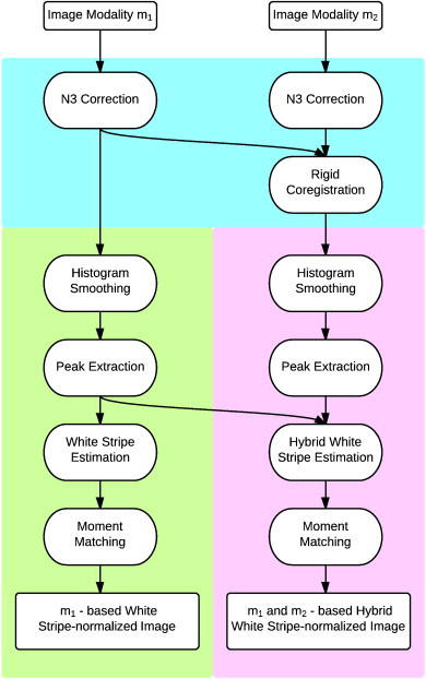
Schematic showing the proposed normalization techniques. The steps shown in the cyan region are standard preprocessing steps, while the green region shows the white stripe normalization algorithm. The bottom right section in purple shows the hybrid white stripe normalization technique.

Our interest lies in developing principled statistical methods for normalizing images to ensure comparability within and across subjects. In the remainder of this paper, we introduce a formal statistical framework and propose statistically principled methods for generalizable and robust inference from large MRI studies. Given the large number of images we intend to normalize (thousands to tens of thousands), the procedure proposed needs to be fully automatic and fast. This requires the robust and rapid identification of the normal-appearing white matter (NAWM) in each subject at each study visit. In previous studies, Shinohara et al. (2011) used a white-matter mask based on the Lesion-TOADS (Shiee et al., 2010) segmentation algorithm. The problem with such an approach is that it can be slow (45 min per image), it requires manual tuning of segmentation parameters, and its performance can be sensitive to heterogeneity in large imaging studies. We suspect that this may be due to the use of unsupervised methods for image segmentation using unnormalized data. To avoid this, we propose a faster and more robust approach.

2.2. Study populations

We first study two large populations consisting of healthy subjects, subjects with mild cognitive impairment (MCI), and subjects with AD. The first is the ADNI database (adni.loni.ucla.edu). In the data analyzed in this paper, we consider 616 adults aged 55 to 90 consisting of cognitively normal older individuals, people with MCI, and people with early AD who were imaged longitudinally at 1427 study visits (1–7 visits per subject). The second source of data was collected by the AIBL study group. AIBL study methodology has been reported previously (Ellis et al., 2009), and 262 cognitively normal older individuals, people with MCI, and people with early AD aged 55 to 90 were imaged longitudinally (1–2 visits per subject) at 442 study visits.

We also consider two studies of multiple sclerosis (MS) from two different centers in the US. The Neuroimmunology Branch of the National Institute for Neurological Disorders and Stroke (NINDS) and the Department of Neurology and Neurosurgery at the Johns Hopkins School of Medicine are simultaneously acquiring MRI for the long-term study of the natural history and treatment of MS. From these ongoing separate studies, we consider 242 (99 from Johns Hopkins and 143 from NINDS) patients with MS scanned under a diverse collection of acquisition protocols and scanners. Clinical summaries of the population of MS subjects studied in this work are described elsewhere (Sweeney et al., 2013b).

2.3. Imaging sequences and preprocessing

From the ADNI and AIBL studies, we consider T1-weighted (T1-w) MP-RAGE and T2-weighted (T2-w) imaging acquired on 1.5 and 3 T scanners according to the standardized protocol (Jack et al., 2008). For the studies of MS at Johns Hopkins and NINDS, we analyze T1-w and T2-w imaging acquired under protocols on 3 T scanners described elsewhere (Sweeney et al., 2013a, 2013b). All image preprocessing was conducted using the Medical Image Processing, Analysis and Visualization (http://mipav.cit.nih.gov) software environment through the Java Image Science Toolkit (Lucas et al., 2010). All images were corrected for spatial inhomogeneity (Sled et al., 1998) and rigidly aligned across modalities at each study visit to the Montreal Neurological Institute template. For performance assessment within tissue types, TOADS (Bazin and Pham, 2007) was used for segmentation of the brain in the AD studies, and LesionTOADS (Shiee et al., 2010) was used in MS studies. These segmentations were not used for any normalization technique described below, but only for performance assessment.

2.4. Methodology

The goal of our method is to minimize the discrepancy between the distributions of intensities f_ijk(⋅) across subjects and visits within tissue classes while respecting SPIN. We call this tissue-specific histogram normalization. We propose to accomplish this by focusing on matching moments of the distribution in a particular reference tissue and appropriately adjusting the intensity distribution in other tissues accordingly. Assume for the moment that, for every subject and visit, we have an area of white matter (a sub-mask of the white matter). Then we can accurately estimate the distribution function f_ij1(x) (say k = 1 for white matter) for each i and j and obtain a normalized estimator that has a mean of zero and a variance of one, ${\displaystyle {\widehat{g}}_{\mathit{ij}1}}\left(x\right)={\sigma }_{\mathit{ij}1}{f}_{\mathit{ij}1}\left({\mu }_{\mathit{ij}1}+{\sigma }_{\mathit{ij}1}x\right)$, where μ_ij1 and σ_ij1 are the mean and standard deviation of f_ij1(x), respectively. An estimator of the normalized histogram across the image using linear normalization with respect to the white-matter distribution is:

$${\displaystyle {\widehat{g}}_{\mathit{ij}}}\left(x\right)={\sigma }_{\mathit{ij}1}{f}_{\mathit{ij}}\left({\mu }_{\mathit{ij}1}+{\sigma }_{\mathit{ij}1}x\right)={\displaystyle \sum _{k=1}^K{w}_{\mathit{ijk}}\left[{\sigma }_{\mathit{ij}1}{f}_{\mathit{ijk}}\left({\mu }_{\mathit{ij}1}+{\sigma }_{\mathit{ij}1}x\right)\right].}$$ (2)

All units are expressed in multiples of standard deviations, σ_ij1, of the white-matter intensities, and zero is the average intensity of white matter. Note that the densities f_ijk(⋅) and weights w_ijk are theoretical and need not be estimated in practice (except for f_ij1(⋅) as described above). This method was used in several papers (Sweeney et al., 2013a; Shinohara et al., 2011), though it was never proposed as a formal normalization procedure and its statistical properties for normalizing other tissues have not been investigated.

Consider a T1-weighted structural MR image, Y_ij(v). The proposed normalization techniques are shown in a flow diagram in Fig. 1. We use NAWM as a reference tissue, since it is the most contiguous brain tissue and therefore least confounded by partial volume averaging and is, by definition, not obviously affected by pathology (leading to conformity to SPIN 5). To identify the distribution of NAWM intensities, we first isolate a rectangle containing the measured intensities within an α = 4 cm section at the center of the head (using a fast rigid alignment to the Montreal Neurological Institute template). The thickness α of this section was chosen empirically (see Fig. A.3 for a sensitivity analysis). We then use a penalized spline smoother (Ruppert et al., 2003), a fully automatic smoothing technique that estimates the smoothing parameter, to estimate the mode μ_ij1^∗ (the largest non-background peak) of the intensity histogram in white matter based on this rectangle. To estimate the variability within NAWM on the raw image, we estimate the standard deviation σ_ij1^∗ of intensities within Ω_i,j,τ = {v : F_ij^− 1[F(μ_ij1^∗) − τ] < Y_ij(v) < F_ij^− 1[F(μ_ij1^∗) + τ]}, which we call the white stripe (where F_ij(x) = ∫ _− ∞^xf_ij(x) dx). Here τ is a quantile tolerance in the original space of intensities. We found several values to work well in practice and used τ = 0.05 after conducting a sensitivity analysis (see Appendix B). The estimation of μ_ij1^∗ and σ_ij1^∗ has been found to be remarkably robust across thousands of images (failure rate < 1%, 15 out of 2109 study visits). If the family of densities f_ij1(v) can be parameterized by two parameters then μ_ij1 = ψ₁(μ_ij1^∗, σ_ij1^∗) and σ_ij1 = ψ₂(μ_ij1^∗, σ_ij1^∗) (proof follows from the method of moments). Thus, matching μ_ij1^∗ and σ_ij1^∗ (estimable directly from the white stripe without prior segmentation) results in matching μ_ij1 and σ_ij1. This process, which we refer to as white stripe normalization, is demonstrated visually for a single image in Fig. 2.

Fig. A.3.

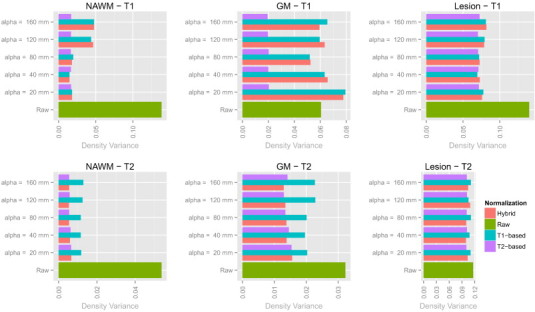
Bar plots showing the Hellinger distance-based variances before and after normalization in the NINDS study for various values of α.

Fig. 2.

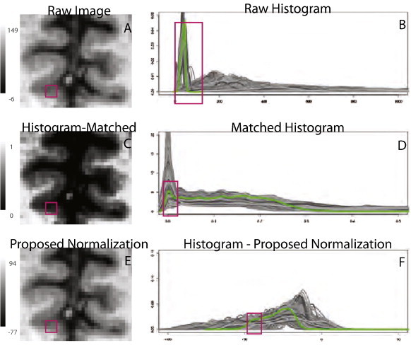
Failure of histogram matching methods. First column: region of interest from patient with MCI shown before (A) and after (C) histogram matching. Red square indicates region of gray matter on raw image that disappears after histogram matching. Second column: histograms (shades of gray indicate different study visits) of the gray matter before (B) and after (D) histogram matching for subjects in ADNI. Note the large proportion of gray matter incorrectly matched to background (zero intensity). The green line shows the histogram for the image shown in the left column. (E) and (F) show the same image and histograms after the normalization proposed in this paper.

For multimodal imaging, including multi-sequence MR imaging acquired in the studies of interest, the above normalization technique does not apply directly. To address this, we first propose the rigid alignment of the multi-modality imaging using standard techniques within each study visit. This robust procedure produces a four-dimensional image Y_ij^(m)(v) for m = 1, …, M where M is the number of modalities acquired. Fortunately, in almost all modern research MRI protocols the acquisition of a high-resolution T1-w image is a key component. Thus, to extend the methods developed above, we consider the use of the white stripe method on the T1 image Y_ij⁽¹⁾(v) to estimate the white stripe Ω_i,j,τ⁽¹⁾. Then, for each modality m, we estimate the white stripe moments μ_ij1^(m) ∗ and σ_ij1^(m) ∗. We then normalize each modality by calculating {Y_ij^(m)(v) − μ_ij1^(m) ∗}/σ_ij1^(m) ∗. An alternate approach is to normalize by using our peak-finding algorithm to find the largest non-background mode in the histogram on modality m, and use this to form the white stripe Ω_i,j,τ^(m). Note that this peak does not necessarily correspond to NAWM alone on all imaging modalities; in particular, the white stripe estimation applied directly to T2-weighted imaging yields a mixture of GM and WM intensities since these are similar. This results in good performance for normalization of both tissue classes, but excellent performance for neither. A natural extension of this idea is to normalize using tissue from the white stripe in all classes; that is, normalizing with respect to Ω_i,j,τ^hybrid = ∩ _mΩ_i,j,τ^(m) allows comparability in terms of a more specific definition across modalities. Thus, in the Results section, we compare these three proposed normalization methods: 1) the T1-based white stripe, which normalizes the data based on Ω_i,j,τ⁽¹⁾; 2) the T2-based white stripe, based on Ω_i,j,τ⁽²⁾; and 3) a hybrid white stripe using Ω_i,j,τ^hybrid.

To assess the performance of the various methods described above, we propose a new generalization of variance for probability densities to quantify variability before and after normalization as measure of SPIN 4. From the theory of U-statistics (Hoeffding, 1948), the sample variance ${\displaystyle {\sum }_{\left(l,k\right)\in {\Gamma }^{\ast }}{\displaystyle \int {\left(\sqrt{f_l\left(u\right)}-\sqrt{f_k\left(u\right)}\right)}^2\mathit{du}/2\left|{\Gamma }^{\ast }\right|}}$ where Γ^⁎ is a randomly chosen sufficiently large subset of Γ (for this study we used |Γ^∗| = 2000). Asymptotic properties of our estimated variance of densities follow from standard U-statistic arguments as the number of densities under study increases.

3. Results

All images from the four studies were normalized using the histogram matching-based approach (Shah et al., 2011; Nyul and Udupa, 1999), and the T1-based, T2-based, and hybrid white stripe methods proposed in the Methodology section. Fig. 1 shows how the faulty assumption made by histogram matching of common distributions of tissue throughout the head causes severe mismatching of gray matter (GM) to cerebrospinal fluid (CSF); note how a normal-appearing part of the brain (raw data shown in Fig. 1A) is induced to show massive erosion of GM by histogram normalization (histogram normalized data shown in Fig. 1C). Such failures are crippling to many quantitative studies of anatomical development and etiology. The results from our proposed T1-based normalization method are shown in Fig. 1E and F and demonstrate significant improvement over histogram matching. An additional example for visual inspection is shown in Figs. A.10 and A.12 of the Appendix, and an example of severe erosion in an imaging study with motion artifact after histogram matching is shown in Figs. A.11 and A.13.

Simulations were conducted to validate the performance of the proposed image normalization methodology, and the results are provided in Appendix A. To visually assess the performance of differing normalization methods across the four MRI studies, the histograms of the T1-w and T2-w images are displayed in Fig. 3 for the AD studies and Fig. 4 for the MS studies. Each line corresponds to a study visit where color indicates the study and differing shades are for clarity in illustration. In Fig. 3, the first two columns correspond to the T1-w and T2-w densities in cerebral white matter and the second two correspond to the gray matter. In Fig. 4, the last two columns correspond to white matter lesions.

Fig. 3.

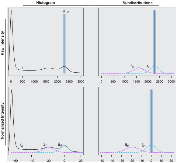
Example of the white stripe normalization procedure. In the top left plot, the raw histogram of a T1-w image is shown. Using a peak-finding algorithm, μ_ij1^∗ and thus Ω_i,j,τ are estimated. In the right column of the figure, Ω_i,j,τ is shown before and after normalization. The density of the intensities in NAWM before (f_ij1) and after normalization $\left({\displaystyle {\widehat{g}}_{\mathit{ij}2}}\right)$ is shown using dashed magenta lines. The bottom left plot shows the histogram after white stripe normalization.

Fig. 4.

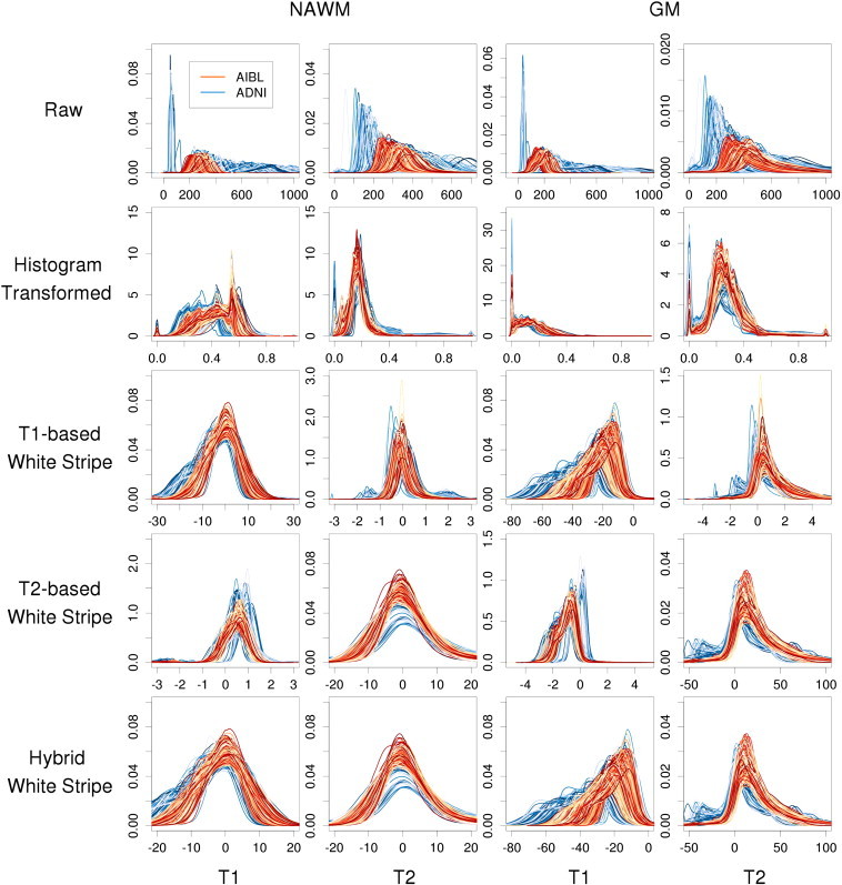
Histograms of intensities before and after normalization by tissue type in two large studies of AD. Rows indicate different normalization methods and columns correspond to MR sequence and anatomical structure.

The results below do not include 15 study visits (0.7%) across the four studies on which our peak-finding algorithm failed. These were identified via manual inspection, and this failure was attributable to very severe chronic MS (2 patients), diffuse vascular white matter disease (5 patients), and high BMI resulting in excess fat in the scalp (5 subjects, mean BMI = 32.4). For obese subjects, standard fast skull-stripping algorithms, such as FSL BET (Smith, 2002), solves these issues associated with excess extracranial fat. Each of these subjects shows that in severe cases of pathology and in some outliers, SPIN 5 may be violated.

The heterogeneity in raw intensities across scans shows variability as expected, even in the ADNI and AIBL studies where protocols were mandated in advance and tightly controlled. The histogram-transformed intensities (second row of Figs. 3 and 4) also show significant variability as well as mismatching as described in Fig. 1. The T1-based white stripe shows good comparability of the NAWM distributions across subjects and visits on the T1-w imaging, but less comparability in the T1-w GM. This is expected due to the partial volume averaging of GM voxels with WM and CSF, and the differential WM to GM contrast ratios across images and protocols. The T2-w NAWM also shows large heterogeneity under the T1-based white stripe normalization, especially in the Hopkins study. The T2-based white stripe shows generally good comparability on the T1-w imaging in both the WM and GM, and especially good comparability on the T2-w imaging. However, the proposed T1-based method shows slightly closer T1-w distributions in the NAWM. Finally, the hybrid method shows similar performance to the T1-based method on T1-w imaging, and near identical performance to the T2-based method on T2-w imaging. In MS lesions, the T1-based and hybrid white stripe methods show moderate comparability across subjects on T1-w imaging. This is likely due to the much greater biological heterogeneity in these regions. The T2-based and hybrid white stripe methods result in good comparability across subjects on T2-w imaging in the Hopkins study, but poor comparability across subjects in the NINDS study likely due to the much larger range in scanning parameters. Figs. A.5–A.7 of the Appendix show the results from the AD studies separated by baseline diagnosis, and Figs. A.8–A.9 show the results from the MS studies separated by lesion load. The white stripe methods perform similarly independent of disease severity.

To assess these comparisons quantitatively, we use the Hellinger distance-based variance proposed in the Methodology section. Our proposed variance measures heterogeneity in a sample of densities; smaller values of this quantity within tissue types indicate better comparability (SPIN 4). Furthermore, lower variance in large heterogeneous imaging studies suggests more replicable measurements (SPIN 2), low sensitivity to the spectrum of biological abnormality (SPIN 5), and low sensitivity to minor noise and artifacts (SPIN 6).

The results from these variance calculations are shown in Fig. 6. The performance of the hybrid white stripe method is superior to other proposed methods in most cases, including the histogram matching method. As noted above in Figs. 4 and 5, the hybrid method shows small variances in the NAWM and WM lesion in all modalities and low variance in the GM on the T2-w imaging. The large variance in the T1-w densities in the GM reflects the nature of the white stripe normalization; if the primary goal of interest is to study GM on T1-w imaging, a normalization targeted specifically to gray matter motivated by the proposed white stripe method might be appropriate.

Fig. 6.

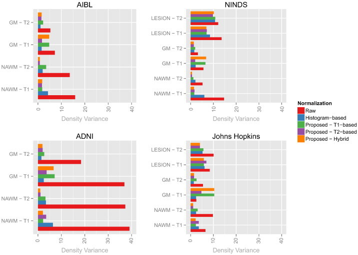
Bar plots showing the Hellinger distance-based variances before and after normalization in the four studies (shorter bars show more similarity in intensity distribution across images). Each plot corresponds to a single study and each bar represents a single tissue class on a particular modality after a normalization (indicated by color).

Fig. 5.

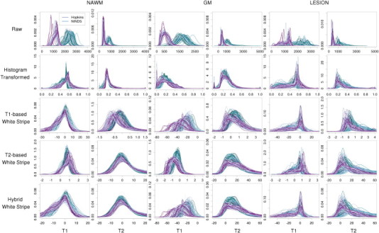
Histograms of intensities before and after normalization by tissue type in two large studies of MS. Rows indicate different normalization methods and columns correspond to MR sequence and anatomical structure.

4. Discussion

We have introduced SPIN, a set of principles for image normalization and an explicit framework based on mixtures of distributions, where each fundamental distribution has a physical interpretation. Although intensity normalization has been acknowledged as crucial for the quantitative analysis of MRI, there are currently no automatic methods for statistical intensity normalization of brain MRI that satisfy the basic requirements of SPIN. In addition, confounding due to acquisition- and subpopulation-related differences across scanners and study sites is more problematic in increasingly more common multi-modality studies that require more complex protocols.

We propose the first methodology for the statistical normalization of neuroimaging that satisfies SPIN. Our methods require less than 5 s of computation time on a standard laptop per MRI scan, making them highly suitable for routine use in clinical practice and research. Using fast, scalable, and fully automatic coarse segmentation techniques, we suggest a simple and robust technique for estimating parameters of the NAWM distribution in an image. These parameters are matched across visits and subjects to yield simple and clear biological interpretations. This approach is robust to artifact and pathology and allows for generalizable inference to large multi-center imaging studies.

Our proposed methodology satisfies SPIN under many circumstances through a subject/visit-specific linear transformation of intensities resulting in the same physical interpretation across subjects and visits. In addition, using information across imaging modalities jointly allows for more precise normalization with similar simple interpretation of units across modalities. Using precursors to this methodology (Sweeney et al., 2013a, 2013b) we have found dramatically improved lesion detection performance cross-sectionally and longitudinally; the methods proposed here promise further improvement in performance and dramatically reduced computational requirements.

Our methods aim to match the intensity of tissues without upsetting the natural balance of tissue intensities. When this is not possible, we characterize how far apart the tissue-specific components are. This approach is fundamentally different from the normalization algorithms common in genomics (for example, see Irizarry et al., 2003), which are dedicated to matching distributions with one component. Instead, we propose intensity normalization approaches for mixtures of densities where each density has a physical interpretation, using a pre-selected reference tissue type. The results from our analyses indicate good comparability across study visits, subjects, study centers, and highly heterogeneous scanning protocols. Although we present our methods in the context of T1-w and T2-w MRI of the brain, our methods may be naturally extended to other imaging modalities used throughout the body. In some scenarios, the coarse segmentation used here may not perform well and alternative segmentation methods may be more appropriate for segmenting a reference tissue.

Although the T1-based method conforms to SPIN, the proposed T2-based method violates SPIN for normalizing T1-w imaging. First, as the relative proportions of WM and GM vary from patient to patient, SPIN 4 is violated. Furthermore, as patients with varying severity of diseases such as AD and MS have varying loss of GM, SPIN 5 does not hold. However, as the distribution of T2-w intensities in the WM and GM are similar, applying the T2-based normalization to the T2-w imaging conforms to SPIN. The hybrid white stripe method, which performs similarly to the modality-specific normalizations on the appropriate images, does not result in any major violations of SPIN and in most cases dramatically improves the comparability of imaging across study visit, subjects, and study protocols.

While the proposed techniques involve the normalization with respect to a particular reference tissue, extensions might involve the normalization of each tissue class individually. However, this would induce dependency on the accuracy of segmentation which may not be desirable in many cases of large imaging databases where segmentation remains difficult. Furthermore, artifacts from patient motion and other sources could be problematic as they are known to affect segmentation, which could then also affect the normalization.

Appendix A. Simulation studies

To investigate the performance of the proposed white stripe normalization techniques, we conducted a series of simulation studies. We used the two-dimensional image template shown in Fig. A.1 and sampled n = 100 subject images using the intensity data generating distribution:

$$Y_i\left(v\right)\sim Z_{\mathit{SHIFT},i}+Z_{\mathit{SCALE},i}^2\cdot \left\{\begin{array}{l}N\left(20,{\sigma }_W\right)\mathrm{for}v\mathrm{in}\mathrm{NAWM}\\ N\left(10+Z_{\mathit{GM},i},{\sigma }_W\right)\mathrm{for}v\mathrm{in}\mathrm{GM}\\ N\left(10+Z_{\mathit{lesion},i}\right),\left({\sigma }_W\right)\mathrm{for}v\mathrm{in}\mathrm{lesion}\\ N\left(10+Z_{\mathit{BG},i}\right),\left({\sigma }_W\right)\mathrm{for}v\mathrm{in}\mathrm{background}\end{array}\right)$$

where Z_SHIFT,i, and Z_SCALE,i ∼ N(0, 1) are latent subject-level whole-image shift and scale random variables, and Z_GM,i, Z_lesion,i, and Z_BG,i ∼ N(0, σ_μ) are latent tissue-specific shifts. We simulate data under the nine scenarios of varying values of the parameters σ_μ and σ_W as shown in Table 1

Table 1.

Parameters used in the simulation study. The parameter σ_μ is the standard deviation of the means across tissue classes across subjects, and σ_W is the standard deviation of intensities within each tissue class.

Simulation setting	σμ	σW
1	0.10	1
2	0.10	2
3	0.10	5
4	0.25	1
5	0.25	2
6	0.25	5
7	0.5	1
8	0.5	2
9	0.5	5

. The performance of the white stripe normalization applied to the raw intensities Y_i(v) is shown in Fig. A.2, and the method performs well throughout. The white stripe normalization shows least benefit in setting 7 for which the variability in means across tissue classes is most similar to the variability within tissue classes; this is a difficult case in which a highly nonlinear normalization would be necessary to improve normalization performance in the GM and lesion tissue classes, and such techniques require further study.

Fig. A.1.

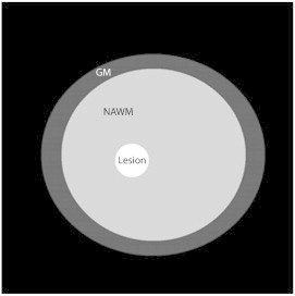
Template image used for simulation experiments. Differing shades of gray indicate different tissue classes.

Fig. A.2.

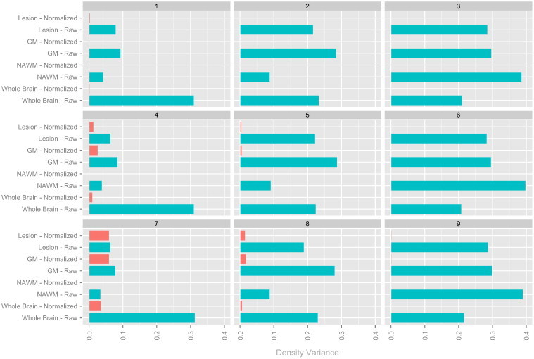
Bar plots showing the Hellinger distance-based variances before and after normalization in the simulation studies (shorter bars show more similarity in intensity distribution across images). Each plot corresponds to a different set of parameters (shown in Table 1) and each bar represents a single tissue class on a particular modality after a normalization (indicated by color, with green indicating raw images and orange indicating white stripe normalized images). Note that the method performs well throughout, but shows least benefit in setting 7 for which the variability in means across tissue classes is most similar to the variability within tissue classes.

Appendix B. Sensitivity analyses for α and τ

To assess the sensitivity of the proposed methodology to the specification of the parameter α, we reanalyzed the data from the MS study at NINDS across a variety of values of α. The results from this analysis are shown in Fig. A.3, and show relative stability in the normalization for the T1-based, T2-based, and hybrid white stripe normalizations for α ranging from 20 mm to 80 mm. We chose to use the 40 mm thickness as it was optimal in the NAWM, and also because differential BMI and other extracerebral tissue factors resulted in poor differentiation of the NAWM peak in some studies for larger thicknesses.

To assess the sensitivity of the proposed methodology to the specification of the parameter τ, we reanalyzed the data from the MS study at NINDS across a variety of values of τ. The results from this analysis are shown in Fig. A.4, and show stability in the normalization for the T1-based, T2-based, and hybrid white stripe normalizations for τ ranging from 1% to 10%. For τ = 20%, the T1-based normalization technique showed less comparable intensities across all tissue classes.

Fig. A.4.

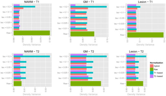
Bar plots showing the Hellinger distance-based variances before and after normalization in the NINDS study for various values of τ.

Appendix C. Supplementary data

Supplementary figures.

References

- Anderson V.M., Schott J.M., Bartlett J.W., Leung K.K., Miller D.H., Fox N.C. Gray matter atrophy rate as a marker of disease progression in AD. Neurobiol. Aging. 2012;33:1194–1202. doi: 10.1016/j.neurobiolaging.2010.11.001. [DOI] [PMC free article] [PubMed] [Google Scholar]
- Bazin P.-L., Pham D.L. Topology-preserving tissue classification of magnetic resonance brain images. IEEE Trans. Med. Imaging. 2007;26:487–496. doi: 10.1109/TMI.2007.893283. [DOI] [PubMed] [Google Scholar]
- Ellis K.A., Bush A.I., Darby D., De Fazio D., Foster J., Hudson P., Lautenschlager N.T., Lenzo N., Martins R.N., Maruff P., Masters C., Milner A., Pike K., Rowe C., Savage G., Szoeke C., Taddei K., Villemagne V., Woodward M., Ames D., AIBL Research Group The Australian Imaging, Biomarkers and Lifestyle (AIBL) study of aging: methodology and baseline characteristics of 1112 individuals recruited for a longitudinal study of Alzheimer's disease. Int. Psychogeriatr. 2009;21(4):672–687. doi: 10.1017/S1041610209009405. [DOI] [PubMed] [Google Scholar]
- Hellier P. Vol. 1. 2003. Consistent intensity correction of MR images. (Image Processing, 2003 ICIP 2003). (I-1109IEEE) [Google Scholar]
- Hoeffding W. A class of statistics with asymptotically normal distribution. Ann. Math. Stat. 1948;19:293–325. [Google Scholar]
- Irizarry R.A., Hobbs B., Collin F. Exploration, normalization, and summaries of high density oligonucleotide array probe level data. Biostatistics. 2003;4:249–264. doi: 10.1093/biostatistics/4.2.249. [DOI] [PubMed] [Google Scholar]
- Jack C.R., Bernstein M.A., Fox N.C. The Alzheimer's disease neuroimaging initiative (ADNI): MRI methods. J. Magn. Reson. Imaging. 2008;27:685–691. doi: 10.1002/jmri.21049. [DOI] [PMC free article] [PubMed] [Google Scholar]
- Jäger F., Deuerling-Zheng Y., Frericks B., Wacker F., Hornegger H. Vision Modeling and Visualization. 2006. A new method for MRI intensity standardization with application to lesion detection in the brain; pp. 269–276. [Google Scholar]
- Leung K.K., Clarkson M.J., Bartlett J.W. Robust atrophy rate measurement in Alzheimer's disease using multi-site serial MRI: tissue-specific intensity normalization and parameter selection. NeuroImage. 2010;50:516–523. doi: 10.1016/j.neuroimage.2009.12.059. [DOI] [PMC free article] [PubMed] [Google Scholar]
- Loizou C.P., Pantziaris M., Seimenis I., Pattichis C.S. Information Technology and Applications Biomedicine, 2009 ITAB 2009. 2009. Brain MR image normalization in texture analysis of multiple sclerosis. (1-5IEEE) [DOI] [PubMed] [Google Scholar]
- Lucas B.C., Bogovic J.A., Carass A. The Java Image Science Toolkit (JIST) for rapid prototyping and publishing of neuroimaging software. Neuroinformatics. 2010;8:5–17. doi: 10.1007/s12021-009-9061-2. [DOI] [PMC free article] [PubMed] [Google Scholar]
- Madabhushi A., Udupa J.K. New methods of MR image intensity standardization via generalized scale. Med. Phys. 2006;33:3426. doi: 10.1118/1.2335487. [DOI] [PubMed] [Google Scholar]
- Madabhushi A., Udupa J.K., Moonis G. Comparing MR image intensity standardization against tissue characterizability of magnetization transfer ratio imaging. J. Magn. Reson. Imaging. 2006;24:667–675. doi: 10.1002/jmri.20658. [DOI] [PubMed] [Google Scholar]
- Meier D.S., Guttmann C.R.G. Time-series analysis of MRI intensity patterns in multiple sclerosis. NeuroImage. 2003;20:1193–1209. doi: 10.1016/S1053-8119(03)00354-9. [DOI] [PubMed] [Google Scholar]
- Nyul L.G., Udupa J.K. On standardizing the MR image intensity scale. Magn. Reson. Med. 1999;42:1072–1081. doi: 10.1002/(sici)1522-2594(199912)42:6<1072::aid-mrm11>3.0.co;2-m. [DOI] [PubMed] [Google Scholar]
- Nyul L.G., Udupa J.K., Zhang X. New variants of a method of MRI scale standardization. IEEE Trans. Med. Imaging. 2000;19:143–150. doi: 10.1109/42.836373. [DOI] [PubMed] [Google Scholar]
- Ruppert D., Wand M.P., Carroll R.J. Cambridge University Press; 2003. Semiparametric Regression. [DOI] [PMC free article] [PubMed] [Google Scholar]
- Shah M., Xiao Y., Subbanna N. Evaluating intensity normalization on MRIs of human brain with multiple sclerosis. Med. Image Anal. 2011;15:267–282. doi: 10.1016/j.media.2010.12.003. [DOI] [PubMed] [Google Scholar]
- Shiee N., Bazin P.L., Ozturk A., Reich D.S., Calabresi P.A., Pham D.L. A topology-preserving approach to the segmentation of brain images with multiple sclerosis lesions. NeuroImage. 2010;49:1524–1535. doi: 10.1016/j.neuroimage.2009.09.005. [DOI] [PMC free article] [PubMed] [Google Scholar]
- Shinohara R.T., Crainiceanu C.M., Caffo B.S., Gaitán M.I., Reich D.S. Population-wide principal component-based quantification of blood–brain-barrier dynamics in multiple sclerosis. NeuroImage. 2011;57:1430–1446. doi: 10.1016/j.neuroimage.2011.05.038. [DOI] [PMC free article] [PubMed] [Google Scholar]
- Sled J.G., Zijdenbos A.P., Evans A.C. A nonparametric method for automatic correction of intensity nonuniformity in MRI data. IEEE Trans. Med. Imaging. 1998;17:87–97. doi: 10.1109/42.668698. [DOI] [PubMed] [Google Scholar]
- Smith S.M. Fast robust automated brain extraction. Hum. Brain Mapp. 2002;17:143–155. doi: 10.1002/hbm.10062. [DOI] [PMC free article] [PubMed] [Google Scholar]
- Sweeney E.M., Shinohara R.T., Shea C.D., Reich D.S., Crainiceanu C.M. Automatic lesion incidence estimation and detection in multiple sclerosis using multisequence longitudinal MRI. Am. J. Neuroradiol. 2013;34(1):68–73. doi: 10.3174/ajnr.A3172. [DOI] [PMC free article] [PubMed] [Google Scholar]
- Sweeney E.M., Shinohara R.T., Shiee N. OASIS is Automated Statistical Inference for Segmentation, with applications to multiple sclerosis lesion segmentation in MRI. NeuroImage Clin. 2013;34:68–73. doi: 10.1016/j.nicl.2013.03.002. [DOI] [PMC free article] [PubMed] [Google Scholar]
- Wang L., Lai H.M., Barker G.J., Miller D.H., Tofts P.S. Correction for variations in MRI scanner sensitivity in brain studies with histogram matching. Magn. Reson. Med. 1998;39:322–327. doi: 10.1002/mrm.1910390222. [DOI] [PubMed] [Google Scholar]
- Weisenfeld N.L., Warfield S.K. Biomedical Imaging: Nano to Macro, 2004 IEEE International Symposium on. 2004. Normalization of joint image-intensity statistics in MRI using the Kullback–Leibler divergence. (101–104IEEE) [Google Scholar]
Associated Data
This section collects any data citations, data availability statements, or supplementary materials included in this article.
Supplementary Materials