Inferring Aberrant Signal Transduction Pathways in Ovarian Cancer from TCGA Data

Abstract

This paper concerns a new method for identifying aberrant signal transduction pathways (STPs) in cancer using case/control gene expression-level datasets, and applying that method and an existing method to an ovarian carcinoma dataset. Both methods identify STPs that are plausibly linked to all cancers based on current knowledge. Thus, the paper is most appropriate for the cancer informatics community. Our hypothesis is that STPs that are altered in tumorous tissue can be identified by applying a new Bayesian network (BN)-based method (causal analysis of STP aberration (CASA)) and an existing method (signaling pathway impact analysis (SPIA)) to the cancer genome atlas (TCGA) gene expression-level datasets. To test this hypothesis, we analyzed 20 cancer-related STPs and 6 randomly chosen STPs using the 591 cases in the TCGA ovarian carcinoma dataset, and the 102 controls in all 5 TCGA cancer datasets. We identified all the genes related to each of the 26 pathways, and developed separate gene expression datasets for each pathway. The results of the two methods were highly correlated. Furthermore, many of the STPs that ranked highest according to both methods are plausibly linked to all cancers based on current knowledge. Finally, CASA ranked the cancer-related STPs over the randomly selected STPs at a significance level below 0.05 (P = 0.047), but SPIA did not (P = 0.083).

Introduction

Microarray technology is providing us with increasingly abundant gene expression-level datasets. For example, the cancer genome atlas (TCGA) makes available gene expression-level data on cases and controls in five different types of cancer. Translating the information in these data into a better understanding of underlying biological mechanisms is of paramount importance to identifying therapeutic targets for cancer. In particular, if the data can inform us as to whether and how a signal transduction pathway (STP) is altered in the cancer, we can investigate targets on that pathway.

An STP is a network of intercellular information flow initiated when extracellular signaling molecules bind to cell-surface receptors. The signaling molecules become modified, causing a change in their functional capability and affecting a change in the subsequent molecules in the network. This cascading process culminates in a cellular response. Consensus pathways have been developed based on the composite of studies concerning individual pathway components. Figure 1 shows a portion of the signaling pathway of human primary naive CD4 T cells, downstream from CD3, CD28, and LFA-1 activation. Kyoto Encyclopedia of Genes and Genomes (KEGG) pathway¹ is a collection of manually drawn pathways representing our knowledge of the molecular interaction and reactions for about 136 pathways. Signaling pathways are not stand alone, but rather it is believed there is inter-pathway communication.²

Figure 1.

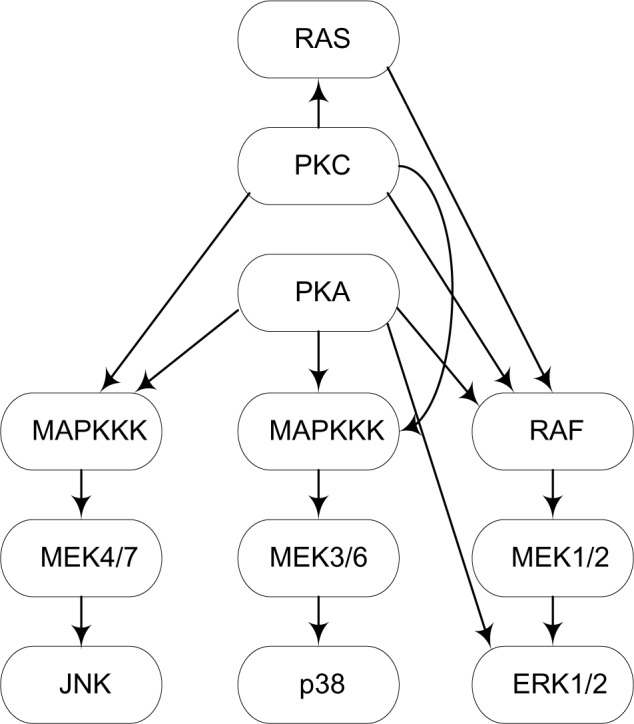
A portion of the STP of human primary naive CD4 T cells, downstream from CD3, CD28, and LFA-1 activation.

Many aberrant STPs have been associated with various cancers.^3–9 For example, we now know that the ErbB, PI3K-Akt, and Wnt pathways are associated with breast cancer. To develop optimal treatments for cancer patients, it is important to discover which STPs are implicated in a cancer or cancer-subtype.

The phosphorylation activity state of each protein in an STP corresponds to the information flow on the STP. However, protein phosphorylation assays are slow, relatively expensive, and can be performed for a tiny but important fraction of the genome. Protein expression level (abundance) is correlated with activity, and gene expression level (mRNA abundance) is associated with protein abundance (correlation coefficient of 0.4–0.6). So, it seems gene expression data should be loosely correlated with activity. Furthermore, as mentioned above, microarray technology is providing us with increasingly abundant gene expression-level datasets. So, researchers developed techniques that investigate which STPs are implicated in a cancer by analyzing gene expression datasets. Initially, techniques such as over-representation analysis^10–12 were employed. These techniques simply determine which genes are differentially expressed in the sample groups. Such methods ignore the topology of the network, and so do not account for key biological information. That is, if a pathway is activated through a single receptor and that protein is not produced, the pathway will be severely impacted. However, a protein that appears downstream may have a limited effect on the pathway. Recently, researchers have developed methods that account for the topology of an STP when analyzing gene expression data to determine whether the STP is implicated in a cancer.^13–15 Signaling pathway impact analysis (SPIA)¹³ is a software package (http://bioinformaticsprb.med.wayne.edu/SPIA) that analyzes gene expression data to identify whether a signaling network is relevant in a given condition that combines over-representation analysis with a measurement of the perturbation measured in a pathway.

However, the correlation of gene expression with activity is not well established. Some studies show that protein expression level (abundance) is often not positively correlated with activity¹⁶ and that gene expression level is often not correlated with protein abundance.¹⁷ Thus, gene expression levels might at most be loosely correlated with activity, which means that the causal structure of an STP might not be represented by the relationships among gene expression levels. More fundamentally, it remained an open question as to whether there even are causal relationships among the gene expression levels of genes coding for proteins on an STP. Neapolitan et al.¹⁸ investigated this question. Specifically, they used a Bayesian network (BN) model to study whether the expression levels of genes that code for proteins on a given STP are causally related and whether this causal structure is altered when the STP is involved in a particular cancer. The results of their study supported that there is a causal structure and that it is altered.

The technique used in the investigation in Ref. 18 provides us with a new method for analyzing whether an STP is implicated in a cancer using gene expression data. In this paper, we present this technique. Then we apply both this technique and SPIA¹³ to the analysis of the ovarian carcinoma dataset provided by TCGA. We obtained highly correlated results using the two methods, and we identified biologically plausible STPs as being the ones to be most likely implicated in ovarian carcinoma.

Method

As our method applies BNs to modeling STPs, we first review BNs.

BNs

A BN^19–21 consists of a directed acyclic graph (DAG) G = (V,E) whose nodeset V contains random variables, and whose edges E represent relationships between the random variables, the prior probability distribution of every root variable in the DAG, and the conditional probability distribution of every non-root variable given each set of values of its parents. Often the DAG is a causal DAG, which is a DAG containing the edge X→Y only if X is a direct cause of Y.¹⁹ The probability distribution of the variables in a BN must satisfy the Markov condition, which states that each variable in the network is probabilistically independent of its nondescendents conditional on its parents.

Figure 2 shows a BN representing the causal relationships among a subset of the variables related to lung cancer. Using this BN, we can determine conditional probabilities of interest using a BN inference algorithm.¹⁹ For example, we can determine P(L = yes|H = yes, X = yes, T = no).

Figure 2.

A BN containing a subset of the variables related to lung cancer.

A BN DAG model consists of a DAG G = (V,E) where V is a set of random variables, and a parameter set θ whose members determine conditional probability distributions for G, but without numerical assignments to the parameters. The task of learning a BN DAG model from data is called model selection.

In the constraint-based approach,²² we learn a DAG model from the conditional independencies that the data suggested are present in the generative probability distribution P. In the score-based approach, we assign a score to a DAG based on how well the DAG fits the data. The Bayesian score is the probability of the Data given the DAG model.²³ A popular variant of this score is the Bayesian Dirichlet equivalent uniform (BDeu) score.²⁴ If the set of variables in DAG model G is {X₁, X₂, …, X_n}, this score is as follows:

$$P(Data|G)={\displaystyle \prod _{i=1}^n{\displaystyle \prod _{j=1}^{q_i}\frac{\Gamma (\alpha /q_i)}{\Gamma (\alpha /q_i+{\displaystyle {\sum }_{k=1}^{r_i}{s}_{ijk}})}{\displaystyle \prod _{k=1}^{r_i}\frac{\Gamma (\alpha /(r_i{q}_i)+s_{ijk})}{\Gamma (\alpha /(r_i{q}_i))}}}}$$ (1)

where α is a parameter called the prior equivalent sample size, r_i is the number of states of X_i, q_i is the number of different instantiations of the parents of X_i, and s_ijk is the number of times in the data that X_i took its kth value when the parents of X_i had their jth instantiation.

When learning a DAG model from data, we can only learn a Markov equivalence class of DAG models rather than a unique DAG model. Two DAGs are called Markov equivalent if they entail the same conditional independencies.¹⁹ For example, the DAGs X → Y→ Z and X ← Y ← Z are Markov equivalent.

Many biological processes have been modeled using BNs including molecular phylogenetics,²⁵ gene regulatory networks,^26–28 genetic linkage,²⁹ genetic epistasis,^30–34 and STPs.^35–39

STPs modeled as BNs

If we represent the phosphorylation activity state of each protein in an STP by a random variable and draw an arc from X to Y if there is an edge from protein X to protein Y in the STP, then we are modeling the STP as a BN. For this BN to represent the joint probability distribution of the random variables, the Markov condition must be satisfied. Woolf et al.³⁸ argue that steady-state concentrations should satisfy this condition. For example, in Figure 1 the phosphorylation activity of MEK1/2 should be dependent on the phosphorylation activity of PKA because the activity of PKA affects the activity of RAF, which in turn affects the activity of MEK1/2. However, once we know the phosphorylation activity of RAF, the implication link is broken, which is what the Markov condition entails. Sachs³⁷ performed a proof of principle study concerning this conjecture, and found that it is true.

Causal analysis of STP aberration (CASA)

In what follows for simplicity we will say that a gene coding for a protein on an STP is on the STP itself. We assume we have two sets of data. The first set contains the gene expression levels of all (or at least most) genes in a set of cases (tumors) and the second set contains the gene expression levels of all genes in a set of controls. Let X be an STP we are investigating, Data₁ be the data concerning cases for genes on X, and Data₂ be the data concerning controls for genes on X.

There are two models. Model M_A represents that the same causal structure (BN) is generating both Data₁ and Data₂. In this case, the two datasets can be considered as coming from the same population and therefore combined. Model M_B represents that two different causal structures (BNs) are generating the data. We compute the log Bayes factor of model M_B relative to model M_A as follows. We first compute

$$\begin{array}{c}P(Data|M_A)={\displaystyle \sum _{g}P(Dat{a}_1,Dat{a}_2|g)P(g|M_A)}\\ =\frac{1}{m}{\displaystyle \sum _{g}P(Dat{a}_1,Dat{a}_2|g)}\end{array}$$ (2)

$$\begin{array}{l}P(Data|M_B)=\left({\displaystyle \sum _{g}P(Dat{a}_1|g)P(g|M_B)}\right)\left({\displaystyle \sum _{g}P(Dat{a}_2|g)P(g|M_B)}\right)\\ =\frac{1}{m^2}\left({\displaystyle \sum _{g}P(Dat{a}_1|g)}\right)\left({\displaystyle \sum _{g}P(Dat{a}_2|g)}\right)\end{array}$$ (3)

where m is the number of possible DAG models containing the variables and g is a variable whose value can be any DAG model. In these computations, we are summing over all DAG models according to the law of total probability (model averaging), and we are assuming all DAG models are equiprobable. The likelihoods are computed using the BDeu score (Equation 1). As there are an intractable number of models, we do approximate model averaging using Markov Chain Monte Carlo (MCMC) as described in Ref. 19. Next, we compute the log Bayes factor K as follows:

$$K=\ln \left(\frac{P(Data|M_B)}{P(Data|M_A)}\right)$$ (4)

The larger the value of K, the more the data indicate that the causal structure of STP X is altered in the tumorous tissue. In our investigations, we approximate the Bayes factor by approximately learning the most likely model and then use the Bayesian information criteria (BIC) to approximate the probability of the data given that model. In the limit, the BIC and the BDeu score (Equation 1) choose the same model.¹⁹

We call the method CASA.

Jiang et al.¹⁸ used Equations (2) and (3) to analyze 5 STPs associated with breast cancer, 10 STPs associated with other cancers, and 10 randomly chosen STPs, using a breast cancer gene expression-level dataset containing 529 cases and 61 controls. They obtained significant results indicating that K (Equation 4) is larger in the cancer-related STPs than in the randomly chosen ones. These results support that the causal structure is altered in the cancer-related pathways. However, the possibility exists that these significant results were obtained simply because the genes are over or under expressed in cancer-related STPs, and the causal structure is not relevant. To test this possibility, they redid the study with all BNs constrained to having no causal edges. They obtained results that had no significance at all. Hence, their overall results support that there is an underlying causal structure among expression levels of genes on an STP and that this causal structure is altered when an STP is involved in cancer. These results indicate that CASA should be able to effectively identify cancer-related STPs.

Application to ovarian cancer

TCGA makes available datasets concerning breast cancer, colon adenocarcinoma, glioblastoma, lung squamous cell carcinoma, and ovarian carcinoma. Each dataset contains data on the expression levels of 17,814 genes in cases (tumorous tissue) and controls (non-tumorous tissue). Table 1 shows the number of cases and controls in each of these datasets.

Table 1.

The number of cases and controls in the five TCGA datasets.

DATASET	# CASES	# CONTROLS
breast cancer	530	62
colon adenocarcinoma	156	20
glioblastoma	596	11
lung squamous cell carcinoma	156	0
ovarian carcinoma	591	9

These datasets are highly unbalanced in that there are many more cases that controls. Difficulties can occur with unbalanced datasets. For example, predictive accuracy, a method often used for evaluating the performance of a classifier, is not appropriate when the data are unbalanced.⁴⁰ However, our application is discovery, not prediction. The BDeu score, which we employ, automatically incorporates both the number of cases and controls into the resultant score. Too few data items would make it more difficult to distinguish models, but not produce an inappropriate measure. Furthermore, to increase the number of controls, we used the controls from all five datasets, resulting in a total of 102 controls.

We investigated the ovarian carcinoma dataset. We analyzed 20 cancer-related STPs to see which ones the data indicate are involved in ovarian cancer. We also analyzed six arbitrary STPs to see whether STPs involved in cancer in general have more implicating scores than arbitrary STPs. These pathways were selected at random from the KEGG pathways list after removing the cancer-related pathways. The STPs analyzed appear in Table 2.

Table 2.

The STPs analyzed using the TCGA ovarian carcinoma dataset.

CANCER PATHWAYS	RANDOM PATHWAYS
P13k	Polycystic Liver Disease Protein Proc. in Endo. Ret.
Wnt	Alpha-1-antitrypsin deficiency_Comp. and Coag. Cascades13
ErbB	Viral Myocarditis
Notch	Salivary Secretion
Hedgehog	Type I Diabetes Mellitus
LUSC-Cell_Cycle Cancer	Type II Diabetes Mellitus
GBM_Ras Cancer
Small Cell Lung Cancer
Nasopharyngeal Cancer_Viral Carc.
Chronic Myeloid Leukemia
GBM_TGF Cancer
Glioma Cancer
Malignant Melanoma
Pancreatic Cancer
LUSC_p53 Cancer
Non-Small Cell Lung Cancer
Colorectal Cancer
LUSC_mTOR Cancer
Thyroid Cancer
Bladder Cancer

Using the KEGG database, we identified all the genes related to each of the 26 pathways. We extracted gene expression profiles for the 591 ovarian carcinoma cases and 102 controls in the TCGA database. By mapping the gene names of the genes in the gene sets identified using KEGG pathways and the gene names in TCGA data, we were able to extract the gene expression profiles for each of the 26 pathways for the 591 cases and 102 controls. All expression levels were discretized to values low, medium, and high using the equal width discretization technique, which discretizes the data into partitions of K equally sized intervals (K = 3 in our application).

Using the resultant datasets, we used CASA to learn Bayes factors and SPIA to determine P-values for the 26 pathways. We used the BN learning package HUGIN⁴¹ to approximately learn the most probable DAG models and to calculate the BICs. We obtained SPIA from http://bioinformaticsprb.med.wayne.edu/SPIA.

Results

Table 3 shows the results for CASA, and Table 4 shows the results for SPIA. The P-values for CASA were obtained by making the null hypothesis that the log Bayes factor is ≤0, assuming a normal distribution, and approximating the variance by the variance of the observed log Bayes factors.

Table 3.

The CASA results for the STPs analyzed using the TCGA ovarian carcinoma dataset.

PATHWAY	LOG BAYES FACTOR	P-VALUE
P13k	7924	0.0000007
GBM_Ras Cancer	4389	0.002
Nasopharyngeal Cancer_Viral Carcinogenesis	3621	0.009
LUSC-Cell_Cycle Cancer	3122	0.021
Wnt	3060	0.023
Polycystic Liver Disease_Protein Processing in Endoplasmic Reticulum	2768	0.035
Small Cell Lung Cancer	1949	0.102
ErbB	1833	0.116
Chronic Myeloid Leukemia	1761	0.125
GBM_TGF Cancer	1703	0.133
Glioma Cancer	1619	0.146
Malignant Melanoma	1587	0.151
Pancreatic Cancer	1531	0.159
Salivary Secretion	1494	0.165
LUSC_p53 Cancer	1389	0.183
Alpha-1-antitrypsin deficiency_Complement and Coagulation Cascades13	1386	0.183
Non-Small Cell Lung Cancer	1313	0.196
Colorectal Cancer	1310	0.197
LUSC_mTOR Cancer	1224	0.213
Hedgehog	1147	0.227
Viral Myocarditis	1031	0.251
Bladder Cancer	1004	0.257
Notch	1003	0.257
Type II Diabetes Mellitus	924	0.274
Thyroid Cancer	642	0.338
Type I Diabetes Mellitus	332	0.414

Table 4.

The SPIA results for the STPs analyzed using the TCGA ovarian carcinoma datasets.

PATHWAY	P-VALUE
P13k	0.00005
Glioma Cancer	0.001
ErbB	0.003
GBM_Ras Cancer	0.013
Malignant Melanoma	0.02
Pancreatic Cancer	0.039
LUSC-Cell_Cycle Cancer	0.051
Chronic Myeloid Leukemia	0.147
LUSC_p53 Cancer	0.147
Notch	0.244
Viral Myocarditis	0.253
Salivary Secretion	0.286
Wnt	0.297
Bladder Cancer	0.338
Type II Diabetes Mellitus	0.378
Colorectal Cancer	0.435
LUSC_mTOR Cancer	0.459
Small Cell Lung Cancer	0.462
Polycystic Liver Disease_Protein Processing in Endoplasmic Reticulum	0.469
Nasopharyngeal Cancer_Viral Carcinogenesis	0.535
Thyroid Cancer	0.644
Type I Diabetes Mellitus	0.732
Alpha-1-antitrypsin deficiency_Complement and Coagulation Cascades13	0.753
Non-Small Cell Lung Cancer	0.776
Hedgehog	0.814
GBM_TGF Cancer	0.906

Notice that in both tables, the cancer-related pathways in general are near the top. Based on a two-sample t-test, the cancer-related pathways scored higher (larger K values for CASA and smaller P-values for SPIA) than the noncancer pathways at the 0.047 level for CASA and at the 0.083 level for SPIA. Also, the P-values for the two methods are highly correlated (correlation coefficient = 0.405; P = 0.040).

We combined the P-values using Brown’s⁴² modification of Fisher’s method because both CASA and SPIA analyzed the same dataset and therefore we do not have independence. The combined P-values appear in Table 5. In this table, we show whether CASA and SPIA individually found each STP noteworthy, where by noteworthy we mean a P-value no larger than 0.05.

Table 5.

The combined results for the STPs analyzed using the TCGA ovarian carcinoma dataset. There is an X in the far right columns if CASA or SPIA separately found the STP noteworthy.

PATHWAY	COMBINED P-VALUE	CASA NOTEWORTHY	SPIA NOTEWORTHY
P13k	0.000	X	X
GBM_Ras Cancer	0.005	X	X
Glioma Cancer	0.012		X
ErbB	0.018		X
LUSC-Cell_Cycle Cancer	0.032	X	X
Malignant Melanoma	0.055		X
Nasopharyngeal Cancer_Viral Carcinogenesis	0.069	X
Pancreatic Cancer	0.078		X
Wnt	0.082	X
Polycystic Liver Disease_Protein Proc. in Endo. Reticulum	0.128	X
Chronic Myeloid Leukemia	0.136
LUSC_p53 Cancer	0.164
Salivary Secretion	0.217
Small Cell Lung Cancer	0.217
Notch	0.250
Viral Myocarditis	0.252
Colorectal Cancer	0.292
Bladder Cancer	0.295
LUSC_mTOR Cancer	0.313
Type II Diabetes Mellitus	0.321
GBM_TGF Cancer	0.348
Alpha-1-antitrypsin deficiency_Comp. and Coag. Cascades13	0.371
Non-Small Cell Lung Cancer	0.390
Hedgehog	0.431
Thyroid Cancer	0.467
Type I Diabetes Mellitus	0.551

Many of the results obtained are plausible according to current knowledge. PI3 K, which is “probably one of the most important pathways in cancer metabolism and growth,”⁴³ has P-value essentially equal to 0 based on each method individually and based on the combined results. Furthermore, PI3 K, Ras, ErbB, and Wnt, all of which rank high, are known players in normal growth regulation and deregulation in cancer cells.

Discussion

We developed CASA, which is a BN-based method for investigating whether STPs are implicated in cancer using case–control gene expression datasets. We applied both CASA and another topology-based method, SPIA, to the TCGA ovarian carcinoma dataset to analyze 20 cancer-related STPs and 6 randomly selected STPs. The results of the two methods were highly correlated. CASA ranked the cancer-related STPs over the randomly selected STPs at a significance level below 0.05 (P = 0.047) but SPIA did not (P = 0.083). Furthermore, several of the STPs that ranked highest are linked to all cancers based on current knowledge.

These results open up avenues for future research. In particular, we can analyze all 136 pathways in KEGG pathway with the purpose of identifying undiscovered pathways related to ovarian cancer. This analysis will require a good deal of manual effort to develop the individual STP datasets from the manually drawn pathways and the TCGA datasets. Second, we can analyze the remaining four cancers in the TCGA datasets, and perform a pan cancer analysis, looking for STPs involved across all cancers.

Conclusion

We conclude that our study supports that both CASA and SPIA can identify aberrant STPs in cancer using case/control gene expression-level data. These results open up avenues for discovering cancer-related STPs across different types of cancers.

REFERENCES

- 1.KEGG PATHWAY. 2014. Available at http://www.genome.jp/kegg/pathway.html.
- 2.Ideker T, Galitski T, Hood L. A new approach to decoding life: systems biology. Annu Rev Genomics Hum Genet. 2001;2:343–72. doi: 10.1146/annurev.genom.2.1.343. [DOI] [PubMed] [Google Scholar]
- 3.Ciriello G, Cerami E, Sander C, Schultz N. Mutual exclusivity analysis identifies oncogenic network modules. Genome Res. 2012;22(2):398–406. doi: 10.1101/gr.125567.111. [DOI] [PMC free article] [PubMed] [Google Scholar]
- 4.Vandin F, Upfal E, Raphael BJ. De novo discovery of mutated driver pathways in cancer. Genome Res. 2012;22(2):375–85. doi: 10.1101/gr.120477.111. [DOI] [PMC free article] [PubMed] [Google Scholar]
- 5.Vandin F, Upfal E, Raphael BJ. Algorithms for detecting significantly mutated pathways in cancer. J Comput Biol. 2011;18(3):507–22. doi: 10.1089/cmb.2010.0265. [DOI] [PubMed] [Google Scholar]
- 6.Zhao J, Zhang S, Wu L-Y, Zhang XS. Efficient methods for identifying mutated driver pathways in cancer. Bioinformatics. 2012;28(22):2940–7. doi: 10.1093/bioinformatics/bts564. [DOI] [PubMed] [Google Scholar]
- 7.Jebar AH, Hurst CD, Tomlinson DC, Johnston C, Taylor CF, Knowles MA. FGFR3 and Ras gene mutations are mutually exclusive genetic events in urothelial cell carcinoma. Oncogene. 2005;24(33):5218–25. doi: 10.1038/sj.onc.1208705. [DOI] [PubMed] [Google Scholar]
- 8.Kurose K, Gilley K, Matsumoto S, Watson PH, Zhou XP, Eng C. Frequent somatic mutations in PTEN and TP53 are mutually exclusive in the stroma of breast carcinomas. Nat Genet. 2002;32(3):355–7. doi: 10.1038/ng1013. [DOI] [PubMed] [Google Scholar]
- 9.Xing M, Cohen Y, Mambo E, et al. Early occurrence of RASSF1 A hypermethylation and its mutual exclusion with BRAF mutation in thyroid tumorigenesis. Cancer Res. 2004;64(5):1664–8. doi: 10.1158/0008-5472.can-03-3242. [DOI] [PubMed] [Google Scholar]
- 10.Drặghici S, Khatri P, Martins RP, Ostermeier GC, Krawetz SA. Global functional profiling of gene expression. Genomics. 2003;81:98–104. doi: 10.1016/s0888-7543(02)00021-6. [DOI] [PubMed] [Google Scholar]
- 11.Subramanian A, Tamayo P, Mootha VK, et al. Gene set enrichment analysis: a knowledge-based approach for interpreting genome-wide expression profiles. Proc Natl Acad Sci USA. 2005;102:15545–50. doi: 10.1073/pnas.0506580102. [DOI] [PMC free article] [PubMed] [Google Scholar]
- 12.Tian L, Greenberg SA, Kong SW, Altschuler J, Kohane IS, Park PJ. Discovering statistically significant pathways in expression profiling studies. Proc Natl Acad Sci USA. 2005;102:13544–9. doi: 10.1073/pnas.0506577102. [DOI] [PMC free article] [PubMed] [Google Scholar]
- 13.Tarca AL, Draghici S, Khatri P, et al. A novel signaling pathway impact analysis. Bioinformatics. 2009;25:75–82. doi: 10.1093/bioinformatics/btn577. [DOI] [PMC free article] [PubMed] [Google Scholar]
- 14.Vaske CJ, Benz SC, Sanborn JZ, et al. Inference of patient-specific pathway activities from multi-dimensional cancer genomic data using PARADIGM. Bioinformatics. 2010;26:i237–45. doi: 10.1093/bioinformatics/btq182. [DOI] [PMC free article] [PubMed] [Google Scholar]
- 15.Ng S, Collisson EA, Sokolov A, et al. PARADIGM-SHIFT predicts the function of mutations in multiple cancers using pathway impact analysis. Bioinformatics. 2012;21(18):640–6. doi: 10.1093/bioinformatics/bts402. [DOI] [PMC free article] [PubMed] [Google Scholar]
- 16.Tsigankov P, Gherardini PF, Helmer-Citterich M, Späth GF, Zilberstein D. Phosphoproteomic analysis of differentiating Leishmania parasites reveals a unique stage-specific phosphorylation motif. J Proteome Res. 2013;12(7):3405–12. doi: 10.1021/pr4002492. [DOI] [PubMed] [Google Scholar]
- 17.Chen G, Gharib TG, Huang CC. Discordant protein and mRNA expression in lung adenocarcinomas. Mol Cell Proteomics. 2002;1(4):304–13. doi: 10.1074/mcp.m200008-mcp200. [DOI] [PubMed] [Google Scholar]
- 18.Neapolitan RE, Xue D, Jiang X. Modeling the altered expression levels of genes on signaling pathways in tumors as causal Bayesian networks. Cancer Inform. 2014;13:1–8. doi: 10.4137/CIN.S13578. [DOI] [PMC free article] [PubMed] [Google Scholar]
- 19.Neapolitan RE. Learning Bayesian Networks. Upper Saddle River, NJ: Prentice Hall; 2004. [Google Scholar]
- 20.Neapolitan RE. Probabilistic Reasoning in Expert Systems. New York, NY: Wiley; 1989. [Google Scholar]
- 21.Pearl J. Probabilistic Reasoning in Intelligent Systems. Burlington, MA: Morgan Kaufmann; 1988. [Google Scholar]
- 22.Spirtes P, Glymour C, Scheines R. Causation, Prediction, and Search. 2nd edition. New York: Springer-Verlag; Boston, MA: MIT Press; 1993. 2000. [Google Scholar]
- 23.Cooper GF, Herskovits E. A Bayesian method for the induction of probabilistic networks from data. Mach Learn. 1992;9:309–47. [Google Scholar]
- 24.Heckerman D, Geiger D, Chickering D. Learning Bayesian networks: the combination of knowledge and statistical data. Mach Learn. 1995;20(3):197–243. [Google Scholar]
- 25.Neapolitan RE. Probabilistic Reasoning in Bioinformatics. Burlington, MA: Morgan Kaufmann; 2009. [Google Scholar]
- 26.Segal E, Pe’er D, Regev A, Koller D, Friedman N. Learning module networks. J Mach Learn Res. 2005;6:557–88. [Google Scholar]
- 27.Friedman N, Linial M, Nachman I, Pe’er D. Using Bayesian networks to analyze expression data. J Comput Biol. 2000;7(3–4):601–20. doi: 10.1089/106652700750050961. [DOI] [PubMed] [Google Scholar]
- 28.Friedman N, Koller K. Being Bayesian about network structure: a Bayesian approach to structure discovery in Bayesian networks. Mach Learn. 2003;50:95–125. [Google Scholar]
- 29.Fishelson M, Geiger D. Optimizing exact genetic linkage computation. J Comput Biol. 2004;11:114–21. doi: 10.1089/1066527041410409. [DOI] [PubMed] [Google Scholar]
- 30.Jiang X, Barmada MM, Visweswaran S. Identifying genetic interactions in genome-wide data using Bayesian Networks. Genet Epidemiol. 2010;34(6):575–81. doi: 10.1002/gepi.20514. [DOI] [PMC free article] [PubMed] [Google Scholar]
- 31.Jiang X, Neapolitan RE, Barmada MM, Visweswaran S. Learning genetic epistasis using Bayesian network scoring criteria. BMC Bioinformatics. 2011;12(89):1471–2105. doi: 10.1186/1471-2105-12-89. [DOI] [PMC free article] [PubMed] [Google Scholar]
- 32.Jiang X, Barmada MM, Cooper GF, Becich MJ. A Bayesian method for evaluating and discovering disease loci associations. PLoS One. 2011;6(8):e22075. doi: 10.1371/journal.pone.0022075. [DOI] [PMC free article] [PubMed] [Google Scholar]
- 33.Jiang X, Neapolitan RE, Barmada MM, Visweswaran S, Cooper GF. A fast algorithm for learning epistatic genomics relationships; Proceedings of American Medical Informatics Association (AMIA). 2010 Annual Fall Symposium; Washington, DC. [PMC free article] [PubMed] [Google Scholar]
- 34.Jiang X, Neapolitan RE. Mining strict epistatic interactions from high-dimensional datasets: ameliorating the curse of dimensionality. PLoS One. 2012;7(10):e46771. doi: 10.1371/journal.pone.0046771. [DOI] [PMC free article] [PubMed] [Google Scholar]
- 35.Sachs K, Gifford D, Jaakkola T, Sorger P, Lauffenburger DA. Bayesian network approach to cell signal pathway modeling. Sci STKE. 2002;148:e38. doi: 10.1126/stke.2002.148.pe38. [DOI] [PubMed] [Google Scholar]
- 36.Sachs K, Perez O, Pe’er D, Lauffenburger DA, Nolan GP. Causal protein-signaling networks derived from multiparameter single-cell data. Science. 2005;308:523–9. doi: 10.1126/science.1105809. [DOI] [PubMed] [Google Scholar]
- 37.Sachs K. Bayesian Network Models of Biological Signaling Pathways [PhD thesis] MIT; 2006. Available at http://hdl.handle.net/1721.1/38865. [Google Scholar]
- 38.Woolf PJ, Prudhomme W, Daheron L, Daley GQ, Lauffenburger DA. Bayesian analysis of signaling networks governing embryonic stem cell fate decisions. Bioinformatics. 2005;21:741–53. doi: 10.1093/bioinformatics/bti056. [DOI] [PubMed] [Google Scholar]
- 39.Pe’er D. Bayesian network analysis of signaling networks: a primer. Sci STKE. 2005;281:l4. doi: 10.1126/stke.2812005pl4. [DOI] [PubMed] [Google Scholar]
- 40.Chawla N. Data mining for imbalanced dataset: an overview. In: Maiman O, Rokach L, editors. Data Mining and Knowledge Discovery Handbook. New York, NY: Springer; 2005. pp. 853–67. [Google Scholar]
- 41.HUGIN. Available at http://www.hugin.com/
- 42.Brown M. A method for combining non-independent, one-sided tests of significance. Biometrics. 1975;31:987–92. [Google Scholar]
- 43.Baselga J. Targeting the phosphoinositide-3 (PI3) kinase pathway in breast cancer. Oncologist. 2011;16(suppl 1):12–9. doi: 10.1634/theoncologist.2011-S1-12. [DOI] [PubMed] [Google Scholar]