Unsupervised Outlier Profile Analysis

Abstract

In much of the analysis of high-throughput genomic data, “interesting” genes have been selected based on assessment of differential expression between two groups or generalizations thereof. Most of the literature focuses on changes in mean expression or the entire distribution. In this article, we explore the use of C(α) tests, which have been applied in other genomic data settings. Their use for the outlier expression problem, in particular with continuous data, is problematic but nevertheless motivates new statistics that give an unsupervised analog to previously developed outlier profile analysis approaches. Some simulation studies are used to evaluate the proposal. A bivariate extension is described that can accommodate data from two platforms on matched samples. The proposed methods are applied to data from a prostate cancer study.

Introduction

Given the availability of high-throughput genomic sequencing technologies, it is possible to measure biological activity on samples in a relatively unbiased and global scale. In such settings, a very common statistical task has been to find genes that are differentially expressed between two experimental conditions. The simplest example is to find genes that are up-or down-regulated in cancerous tissue relative to healthy tissue. The standard approach has been to perform a hypothesis test at each location of the genome measured by the technology. If this involves thousands or millions of locations, then it is obvious that there is an inherent multiple testing problem. There has been an extensive literature on statistical assessment of differential expression in genomic studies (eg, Ge et al.¹). In addition, there has been intensive research done recently on multiple comparison procedures that control the false discovery rate (FDR) that was popularized by Benjamini and Hochberg (B–H).² These authors have argued that since FDR is a more liberal error criterion than the classical familywise error rate (FWER), control of FDR will lead to more rejections of null hypotheses in the multiple testing setting. Scientifically, this corresponds to selecting the significant molecules and is thought to be a useful screening device to identify putative candidate biomarkers.

In most of these studies, differential expression is tested using a test for difference in mean expression; the most commonly used procedure is the two-sample t-test. A more interesting pattern of differential expression was observed by Tomlins et al.³ They identified a gene fusion event in prostate cancer between two transcription factor genes, ERG and ETV1. One line of evidence that led to this observation was that for these genes, only a fraction of samples in one group were overexpressed relative to those in the other group; the remaining samples showed no evidence of differential expression. Tomlins et al.³ developed a ranking method known as COPA (cancer outlier profile analysis) for calculating outlier scores using gene expression data. While their approach did not attempt to assign any measure of significance to the gene scores, Tibshirani and Hastie⁴ and Wu⁵ have shown that significance can be assigned using modifications of two-sample t-tests. Ghosh and Chinnaiyan⁶ synthesized these proposals into a model-based framework for analysis and proposed more non-parametric procedures. These methods all assumed that the statistics of interest were continuous. For data such as those that arise from next-generation sequencing technologies, the methods in the current paper apply if one uses summary measures such as fragments per kilobase of exon per million fragments mapped (FKPM). On the other hand, if the measurements and corresponding statistics used are discrete, then one could apply the work of Ghosh.^7,8 A related proposal, and the one that we will compare in our simulation studies, is based on entropy that was proposed by Kadota et al.⁹ and is abbreviated as ROKU.

All the procedures in the previous paragraph assume that there exist a priori information about samples (eg, healthy versus diseased tissue). It is not as obvious what should be done in the case when no such labels exist. Here, we will revisit the modeling framework of Ghosh and Chinnaiyan⁶ and develop new extensions that deal with the absence of group labels. We explore testing approaches based on the C(α) (C-alpha) principle. This was originally described by Neyman and Scott¹⁰ and applied to a problem of rare variant detection by Neale et al.¹¹ There, the underlying probability model is based on binomial distribution. For the case of gene expression data that is described in the current paper, it will be seen that the C(α) testing procedure poses unique challenges.

Consideration of the C(α) principle will motivate three test statistics, one based on kurtosis, one based on skewness, and the last one based on a combination of skewness and kurtosis. Recall that skewness is defined as the third moment of a distribution, while kurtosis is the fourth moment of the distribution. These have been proposed earlier by D’Agostino et al.¹² We will compare their performance on simulated data in the Simulation Studies section.

Methods

Mixture modeling

We begin by initially considering the genome-wide expression model of Ghosh and Chinnaiyan.⁶ The data consist of (Y_gi,Z_i), where Y_gi is the expression measurement for the gth gene on the ith subject, and Z_i is a binary indicator taking values 0 and 1, i = 1,…,n, g = 1,…,G. In practice, G will be typically much larger than n. The model considered by Ghosh and Chinnaiyan⁶ was the following:

$$\begin{array}{l}{Y}_{gi}|Z_i=0^{\mathrm{i}\underset{~}{\mathrm{n}}\mathrm{d}}{F}_{0g}(y),\\ Y_{gi}|Z_i=1^{\mathrm{i}\underset{\text{~}}{\mathrm{n}}\mathrm{d}}{\pi }_{0g}{F}_{0g}(y)+(1-{\pi }_{0g})F_{1g}(y),\end{array}$$ (1)

where F_0g and F_1g denote the gene-specific distribution functions for the expression in the non-differential and differentially expressed genes, and π_0g denotes the proportion of samples that show no differential expression for gene g.

Ghosh and Chinnaiyan⁶ found several insights from model (1). First, many differential expression proposals, reviewed in Ge et al,¹ can be used to test the null hypothesis that π_0g = 1. In addition, with the exception of the procedures in Ghosh and Chinnaiyan,⁶ most of the procedures were optimal in settings where F_0g has a parametric form, but in fact, this was not necessary. In Ghosh and Chinnaiyan,⁶ non-parametric methods for outlier detection were developed and shown to be quite competitive and sometimes superior to previous proposals for the problem.

All of this development has presumed the existence of Z for the samples. We term this supervised outlier profile analysis, the Z serving as a class label. However, in many instances, Z is not available. One example would be if one only had access to the “-omics” data without it being linked to the appropriate clinical outcomes. In this case, we can no longer specify a model such as (1) because we are unable to condition on Z. However, supposing that we integrate out Z from the model, we get the following model:

$$Y_{gi}{}^{\mathrm{i}\underset{~}{\mathrm{n}}\mathrm{d}}{F}_{0g}(y)+c_g{F}_{1g}(y),$$ (2)

where $c_g=(1-{\pi }_{0_g})(1-P(Z_i=0))$. This is again a two-group mixture model. As described in Ghosh and Chinnaiyan,⁶ a key issue in fitting mixture models of the type (1) and (2) is identifiability of the model using observed data. Identifiability means that given the observed data (here, Y_gi), we can estimate the parameters in the model. For our setting, we cannot estimate c_g, F_0g, and F_1g without making further parametric assumptions on the form of F_0g and F_1g. Thus, we assume here that F_0g and F_1g correspond to cumulative distribution functions from the normal distribution.

This argument started by presuming two subtypes (defined by Z = 0 and Z = 1). Extending this argument theoretically in the situation of infinite subtypes leads to a model of Y_gi as

$$Y_{gi}{}^{\mathrm{i}\underset{\text{~}}{\mathrm{n}}\mathrm{d}}{\displaystyle \sum _{k=0}^{\infty }{c}_k{F}_k(y_{gi};{\theta }_{gk},{\sigma }_{gk}^2),}$$ (3)

where F_k(y, θ, σ) denotes a normal (θ, σ²) cdf:

$$F_k(y,\theta ,{\sigma }^2)={\displaystyle {\int }_{-\infty }^y\frac{1}{\sqrt{2\pi {\sigma }^2}}\exp }\left\{-\frac{{(x-\theta )}^2}{2{\sigma }^2}\right\}\text{dx}.$$

Phrased within this framework, outlier detection for gene g boils down to detection of more than one subtype in model (3). Equivalently, the hypothesis testing problem becomes the following:

H₀: there exists no subtypes for gene g.

In contrast, the alternative hypothesis states that there exists at least one subtype. Note that in the modeling framework of Ghosh and Chinnaiyan,⁶ the alternative is that there are two subtypes. We proceed here with a generalization to infinite subtypes. While this is a theoretical assumption and does not conform to reality, we use this device to motivate the proposed testing procedures in the paper.

C(α) testing

Based on model (3), the null hypothesis H₀ corresponds to testing for no heterogeneity relative to a one-component normal distribution versus the alternative of greater overdispersion. For this setting, a long-standing approach to hypothesis testing in this problem is the C(α) tests, which date back to Neyman and Scott.¹⁰ This class of tests can be motivated in several ways, a survey of which can be found in Chapter 4 of Lindsay.¹³ A recent application of C(α) testing was applied to testing for rare variant effects using genotype case–control data in Neale et al.¹¹ In that problem, the C(α) testing was done based on a binomial model for the data. Mathematically, the C(α) testing procedures correspond to calculating the overdispersion score, defined as the second derivative of the probability density of the data divided by the density. This calculation is done assuming the null hypothesis of one component. The test takes a very simple form, comparing the sample variance to the model-predicted variance for a single binomial distribution. This result extends more generally to one-parameter distributions from the exponential family of distributions. An advantage of C(α) tests is that it does not require specification of a probability density function under the alternative hypothesis; hence, we might expect it to have good power properties over a wide range of alternatives.

For the normal distributions that comprise model (3), this fact no longer holds. This is because of the presence of the mean and variance parameter for each normal distribution. We show in the Appendix that the form of the C(α) test in the normal distribution case is zero if derivatives are taken with respect to μ. By contrast, if derivatives are taken with respect to σ, where μ is treated as a nuisance parameter, we provide the form of the C(α) statistic in the Appendix. As is seen there, the form is relatively complicated.

As discussed in Lindsay,¹³ one intuitive explanation behind the C(α) test is that it is constructed using first- derivative information. The complicated form of the C(α) test in the Appendix suggests the use of estimates of high-order moments. In this article, we consider three tests. The first is based on skewness, defined as the standardized third moment of the distribution. The second is based on kurtosis, defined as the standardized fourth moment of the distribution. The third test combines information of skewness and kurtosis and is called the K2 test; a review of the three tests can be found in D’Agostino et al.¹² The evidence for using these high-order moments can also be an indirect consequence of the discussion in p. 73 of Lindsay,¹³ who describes the behavior for a C(α) test in the normal case to depend on the third and fourth moments of the mixing distribution.

Each of these statistics is applied for every single gene in the dataset to calculate a set of G gene-specific test statistics. To adjust for multiplicity, we will compute P-values corresponding to each statistic and perform an adjustment for multiple comparisons based on the q-value approach of Storey and Tibshirani.¹⁴

Bivariate extension

In many settings, the analyst will have available multiplatform “-omics” data on the same subjects. As a concrete example, we consider copy number and gene expression data so that data from two platforms exist on the same set of samples. Recently, Phillips and Ghosh¹⁵ discussed a bivariate extension of the B–H procedure that can accommodate data from two platforms. They did not consider the proposed test statistics; their algorithm required P-values from the two platforms separately as input. For the sake of completeness, we provide an overview of this two-dimensional modeling approach; the interested reader is referred to Phillips and Ghosh¹⁵ for more details.

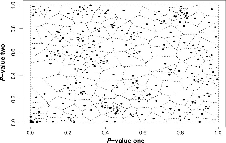
The starting point is the observation that the B–H procedure has a natural interpretation in terms of spacings.¹⁶ In particular, the B–H procedure can be interpreted as comparing the empirical average of the spacings relative to its theoretical expected value, scaled by the FDR. To extend this to a two-dimensional setting, we need a two-dimensional notion of spacings. Jiménez and Yukich¹⁷ argued eloquently for the Voronoi tessellation as one possible extension. A Voronoi tessellation is a partition of the plane generated by an input set of two-dimensional points. In general terms, the tessellation creates a cell around each input consisting of the set of all points closer to that input than to any other. The basic properties of such a tessellation are described by Okabe et al.¹⁸ In the setting of two-dimensional vectors in the unit square, the Voronoi tessellation partitions the unit square. For each p-vector, P_i, the tessellation creates a cell, C_i, consisting of all points closer to P_i than to any other p-vector. An illustration of tessellation for our sample set of points is presented in Figure 1. Voronoi cells have many desirable properties that extend the idea of spacings into the plane. Their area and shape reflect the relative positioning of the input points. For example, clusters of inputs will have smaller cell areas than uniformly distributed inputs. Similarly, if the inputs have correlated components, there will be an increased concentration along the diagonal of the unit square. The Voronoi cells of the inputs close to this diagonal will be smaller than the cells of inputs near the edge of the clustering. In addition, there exists attendant software packages for computing Voronoi tessellations.¹⁹ Our procedure uses the areas of the Voronoi cells generated by the set of p-vectors as a means to account for their relative positions in the unit square. If p-vectors are associated with an alternative hypothesis (and thus present evidence against the null), we expect them to cluster near the origin. It is this clustering at the origin that we hope to detect with our algorithm, as we expect to see very small cell areas associated with these clustered p-vectors.

Figure 1.

An example of Voronoi Tessellation using 200 simulated, two-dimensional data points on the unit square.

Details of the algorithm can be found in Phillips and Ghosh.¹⁵ As recommended by them, we will select the sum ordering scheme for identifying molecules that show significant outlier expression in both platforms. We also note that too much clustering of the P-values near the origin poses computational challenges for the procedure of Phillips and Ghosh¹⁵ and is observed in one of the analyses performed in the prostate cancer data analysis that is described in the Real Data Example: Prostate Cancer section.

Simulation studies

To assess the performance of skewness, kurtosis and K2 tests, we first conducted simulation studies using biologically relevant parameters. We studied two situations. In the first situation, all outlier genes were assumed to be only overexpressed in a few tissues. In the second situation, each outlier gene was both induced and repressed in a few tissue types. In all simulations, we generated gene expression measurements for a total of N genes across T tissue types. We allowed for n₀ genes to have non-preferential expression pattern across tissues and n₁ genes to have tissue preferential expression pattern (N = n₀ + n₁). For the n₀ genes that are not differentially expressed, we took the baseline gene expression to be distributed as normal, which is denoted by $N({\mu }_0,{\sigma }_0^2)$.

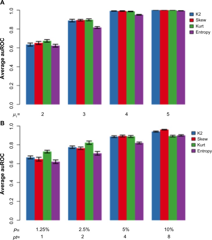
In the situation where outlier genes are only induced in a few tissues, we considered n₁ genes to be induced in pt number of tissues. These n₁ genes had a distribution of $N({\mu }_1,{\sigma }_1^2)$ in the induced tissues and a baseline distribution of $N({\mu }_0,{\sigma }_0^2)$ in other tissues. We compared the performance of the proposed methodology to the entropy-based approach by Kadota et al.⁹ using area under the receiver operating characteristic (ROC) curve (AUC). In term of performance, an AUC value close to 1 indicates good performance, whereas an AUC value of 0.5 indicates poor performance. The simulation results are shown in Figure 2.

Figure 2.

Comparison of AUCs from different simulations. Simulations were carried out with the same set of parameters as in Figure 1 (n₀ = n₁ = 5000, μ₀ = 0, ${\sigma }_0^2=1$, μ₁ = 3, ${\sigma }_0^2=1$, pt = 4), except for that in panel (A) different μ₁ and in panel (B) different pt were used. Values for μ₁ and pt are shown on the x-axis of each panel. The AUC values are averaged over 10 simulations.

Figure 2 shows that all three moment-based methods perform better than the entropy-based approach. Among the moment-based methods, the test based on skewness performs the best, while the K2 test performs better than the kurtosis test when the false-positive rate (FPR) is low.

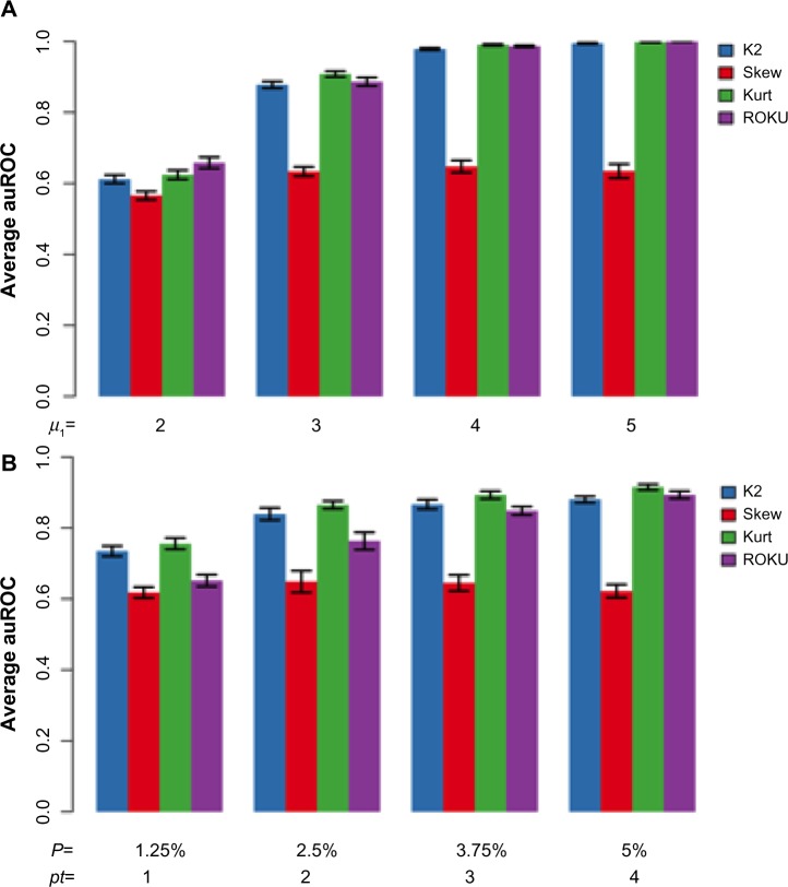
Next, we simulated the situation where each outlier gene is induced and repressed in a few tissues. We generated the baseline distribution for n₀ genes as described above. Each of the n₁ outlier genes had a distribution of $N({\mu }_1,{\sigma }_1^2)$ in pt tissues, a distribution of $\mathit{N}(-{\mathit{\mu }}_1,{\mathit{\sigma }}_1^2)$ in other pt tissues, and a baseline distribution in T − 2 × pt tissues. Figure 3 shows that the entropy method performs better with larger μ₁ and pt, while for smaller μ₁ and pt, the kurtosis test performs the best. The reduced performance of skewness is expected as the simulated outlier genes have symmetrical distribution.

Figure 3.

A comparison of AUCs from different simulations. Simulations were carried out with the same set of parameters as in Figure 2. In panel (A), different μ₁ and in panel (B), different pt were used. Values for μ₁ and pt are shown on the x-axis of each panel. Note that outlier genes are actually differentially expressed in 2 × pt tissues. The AUC values are averaged over 10 simulations.

In practice, of course, the true data-generating distribution is unknown to the analyst. Thus, we would recommend the use of the K2 test that combines information on skewness and kurtosis, as its performance seemed to be quite competitive with the best method for any simulation setting. An open question that is beyond the scope of the current paper is the possibility of constructing data-adaptive weights that can be used to combine the skewness and kurtosis tests in a powerful manner.

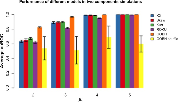
Finally, we did a simulation in which we compared supervised methods such as in Ghosh and Chinnaiyan⁶ to the unsupervised methods developed here. In particular, we compared the B–H approach from Ghosh and Chinnaiyan, which we termed GOBH, to the various methods. Note that GOBH is a supervised algorithm that requires that the samples are labeled as diseased samples and non-diseased samples. The proposed kurtosis, skewness, and K2 tests as well as the entropy-based method (ROKU) are unsupervised models. One would expect that the supervised methods (with labels) outperform the unsupervised methods in general, because a strong hint (ie, the class labels) is given to the supervised method. However, if the labels are not informative, one would expect the supervised methods to perform worse than the unsupervised methods. We performed simulation analyses using the GOBH algorithm with correct sample labels (GOBH) and with shuffled sample labels (GOBH-shuffle). We use the same settings as in Figure 2A but for the purpose of comparisons, we plot everything separately in Figure 4. The results show that the supervised method (GOBH) with correct labels consistently outperforms other methods. However, with shuffled class labels, the supervised method (GOBH-shuffle) shows variable performance with average AUC around 0.5 and is worse than the unsupervised methods.

Figure 4.

Comparison of AUC in supervised (GOBH and GOBH-shuffle) and unsupervised (K2, skewness, kurtosis, ROKU) methods using the settings in Figure 2A.

Real data example: prostate cancer

The real data example features data from copy number and transcript mRNA microarrays, some of which are analyzed in Kim et al.²⁰ We have data on 7534 genes of 47 subjects, 18 of whom have prostate cancer. We show the results of the analysis using the K2 test; similar results were found using the other two methods. We did an initial analysis using all 47 samples; however, no statistically significant genes were found using the procedure of Phillips and Ghosh.¹⁵ This appeared to be because of big differences in expression patterns between the cancer and non-cancer cases. The differences then revealed that the P-values were all clustered near the origin. This rendered the procedure of Phillips and Ghosh¹⁵ to be numerically unstable, as was alluded to in the bivariate extension section.

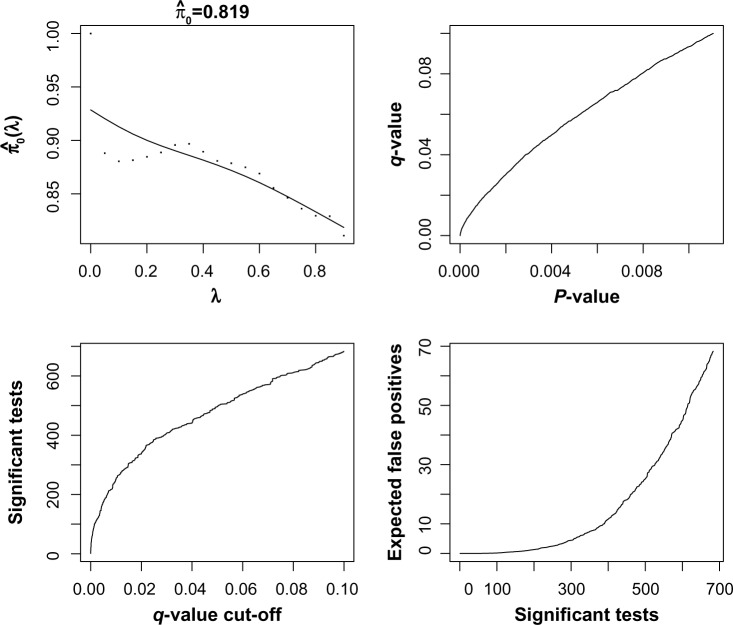
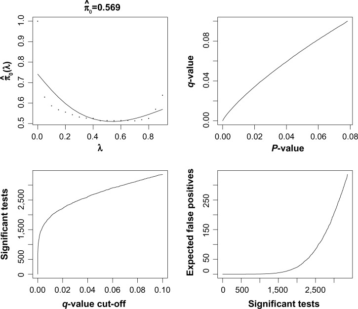
Next, we performed an analysis of the cancer samples only. The goal was to identify genes that show extreme heterogeneity across the cancer subjects, which might be putative cancer biomarkers. First, we applied the analysis with the gene expression only. This is shown in Figure 4. Based on the q-value analysis, we selected 490 genes as significant using an FDR cutoff of 0.05. The q-value analysis estimated about 20% of the genes to show significant expression based on outlier transcript profiles. Next, we repeated the analysis using copy number by itself, as shown in Figure 5. There are many more significant genes that are found using the copy number expression data. About 45% of the genes are called statistically significant using the q-value method. This mirrors what was seen in Kim et al.²⁰ using a supervised statistic. If we were to intersect the results of the individual copy number and gene expression analyses, we would find that 190 genes have an estimated FDR that is less than 0.05 for both platforms.

Figure 5.

Output from q-value function in R for gene expression data using the K2 test. There are 7534 genes on the plot, and statistics were computed using 18 samples.

Next, we show the results of the joint copy number and gene expression analyses using the points in the lower left-corner of Figure 5 corresponding to genes, which will be of interest as they show signal both on the copy number and on the transcript mRNA scale. Applying the procedure of Phillips and Ghosh¹⁵ identifies 734 genes as significantly expressed at an FDR of 0.05. Note that using the information jointly from copy number and transcript mRNA levels using the method of Phillips and Ghosh¹⁵ leads to almost four times as many rejections as the intersection analysis.

Enrichment analysis of the selected genes using DAVID²¹ found pathways such as the cell-cycle pathway, the D4-GDI signaling pathway, and various metabolic pathways as being statistically overrepresented among the selected genes.

Discussion

In this article, we have explored extensions of outlier detection methods in an unsupervised manner. In particular, we found that the C(α) test cannot be used directly here as the way it was for rare variants. However, its application highlights the use of tests for high-order moments as a means of identifying signal in high-throughput genomic data. This complements the work of other authors who have proposed using variability to determine what genes are significantly expressed in high-dimensional data (eg, Refs. 22 and 23). While most of the work has focused on the analysis end, power/sample size considerations are important as well. We have conducted preliminary work that suggests that the proposed methods will have reasonable power for the most existing datasets, but further study is warranted.

The real data example was instructive in that careful selection of samples was needed for application of the statistic. In particular, using all 47 subjects yielded no statistically significant results. This was because of the fact that there were tremendous differences in average measurement intensity for cancer samples and non-cancer samples. With respect to the outlier analysis being considered here, one can view the cancer labels as a confounder. The presence of a confounder can bias the null distribution of the gene-specific test statistics.²⁴

We also point out that the tests proposed here are in line with the “tumor subtyping” paradigm that exists in much of cancer research these days. One practical way these methods could be used is the following. First, gene-wise tests based on the proposed method could be conducted on the tumor samples, and then supervised clustering or classification could be continued based on the identified significant genes. This might help cancer researchers discover novel subtypes and related molecular signatures. However, issues would exist as to the choice of the classifier as well as calibration of the estimated classifier and proper accounting of the variable selection step. This is beyond the scope of the current manuscript.

As pointed out by a referee, the proposed methods are not able to identify the number of subpopulations but are able only to test their presence. An important problem inferentially is to determine the number of subpopulations. A preliminary strategy that we tried and had some success was to filter genes that were statistically significant for kurtosis but not for skewness. However, the operating characteristics of such a strategy remain unknown and deserve further exploration.

Other open questions arise from this work. First, it would be interesting to develop data-adaptive weights to combine information from the skewness and kurtosis estimators in a natural manner. Second, we plan to develop pathway-based approaches for unsupervised outlier detection. Finally, it would be desirable to extend the work of Phillips and Ghosh¹⁵ to accommodate more than one platform as many studies, such as the Cancer Genome Atlas (http://tcga.cancer.gov), are collecting multiple types of “-omics” data on matched samples. These extensions are all currently under investigation.

Figure 6.

Output from q-value function in R for copy number expression data using the K2 test. There are 7534 genes on the plot, and statistics were computed using 18 samples.

Figure 7.

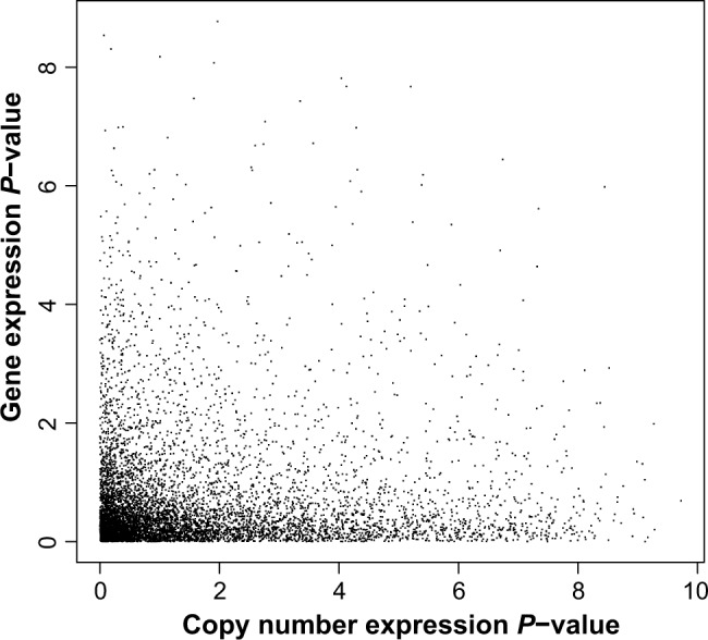
A plot of the P-values from the K2 test for copy number expression (horizontal axis) and from the K2 test for transcript mRNA expression (vertical axis). There are 7534 genes on the plot, and statistics were computed using 18 samples. The axes have been transformed using −log₁₀(P-value).

Appendix

Derivations of C(α) test for N(μ, σ²) distribution

Assume we have a random sample X₁,…,X_n from a normal distribution with mean μ and variance σ². First, we treat μ as the parameter of interest and σ as a nuisance parameter. Using exponential family theory, the C(α) test statistic is given by

$$U(\sigma )={\displaystyle \sum _{i=1}^n{(X_i-\overline{X})}^2}-n{\sigma }^2.$$

If we plug in the maximum likelihood estimate of σ², which is

$${\widehat{\sigma }}^2=\frac{1}{n}{\displaystyle \sum _{i=1}^n{(X_i-\overline{X})}^2},$$

we would get that $U(\widehat{\sigma })$ is identically zero.

We now treat μ as the nuisance parameter and σ as the parameter of interest. The C(α) statistic is given by W = T/V^1/2, where

$$\begin{array}{l}T-\frac{2n}{{\widehat{\sigma }}^2}+\frac{2}{\widehat{\sigma }}{\displaystyle \sum _{i=1}^n{e}^{{(X_i-\overline{X})}^2/{\widehat{\sigma }}^3+{(X_i-\overline{X})}^2/2{\widehat{\sigma }}^2}}+{\displaystyle \sum _{i=1}^n{e}^{-3{(X_i-\overline{X})}^2/{\widehat{\sigma }}^4+(X_i-\overline{X})2/2{\widehat{\sigma }}^2}},\\ V=n+\left[A-\frac{B}{C}\right]\end{array}$$

Here

$$\begin{array}{l}A={{\displaystyle \sum _{i=1}^n\left[\frac{2}{{\widehat{\sigma }}^2}+\frac{2}{{\widehat{\sigma }}^2}{e}^{{(X-\overline{X})}^2/{\widehat{\sigma }}^3+{(X_i-\overline{X})}^2/2{\widehat{\sigma }}^2}+e^{-3{(X_i-\overline{X})}^2/{\widehat{\sigma }}^4+{(X_i-\overline{X})}^2/2{\widehat{\sigma }}^2}\right]}}^2\\ B={\displaystyle \sum _{i=1}^n[-\widehat{\sigma }+e^{{(X_i-\overline{X})}^2(2+\widehat{\sigma })/(2{\widehat{\sigma }}^3)}]\left[\frac{2}{{\widehat{\sigma }}^2}+\frac{2}{\widehat{\sigma }}{e}^{{(X_i-\overline{X})}^2/{\widehat{\sigma }}^3+{(X_1-\overline{X})}^2/2{\widehat{\sigma }}^2}+e^{-3{(X_i-\overline{X})}^2/{\widehat{\sigma }}^4+{(X_i-\overline{X})}^2/2{\widehat{\sigma }}^2}\right]}\\ C={\displaystyle \sum _{i=1}^n{([-\widehat{\sigma }+e^{{(X_i-\overline{X})}^2(2+\widehat{\sigma })/(2{\widehat{\sigma }}^3)}])}^2.}\end{array}$$

$\overline{X}$ is the mean of the sample, and $\widehat{\sigma }$ is the standard deviation. Under the null hypothesis, W is distributed as N(0, 1).

REFERENCES

- 1.Ge Y, Dudoit S, Speed TP. Resampling-based multiple testing for microarray data analysis. Test. 2003;12:1–44. [Google Scholar]
- 2.Benjamini Y, Hochberg Y. Controlling the false discovery rate: a practical and powerful approach to multiple testing. J R Stat Soc B. 1995;57:289–300. [Google Scholar]
- 3.Tomlins SA, Rhodes DR, Perner S, et al. Recurrent fusion of TMPRSS2 and ETS transcription factor genes in prostate cancer. Science. 2005;310:644–8. doi: 10.1126/science.1117679. [DOI] [PubMed] [Google Scholar]
- 4.Tibshirani R, Hastie T. Outlier sums for differential gene expression analysis. Biostatistics. 2007;8:2–8. doi: 10.1093/biostatistics/kxl005. [DOI] [PubMed] [Google Scholar]
- 5.Wu B. Cancer outlier differential gene expression detection. Biostatistics. 2007;8:566–75. doi: 10.1093/biostatistics/kxl029. [DOI] [PubMed] [Google Scholar]
- 6.Ghosh D, Chinnaiyan AM. Genomic outlier profile analysis: mixture models, null hypotheses and nonparametric estimation. Biostatistics. 2009;10:60–9. doi: 10.1093/biostatistics/kxn015. [DOI] [PMC free article] [PubMed] [Google Scholar]
- 7.Ghosh D. Discrete nonparametric algorithms for outlier detection with genomic data. J Biopharm Stat. 2010;20:193–208. doi: 10.1080/10543400903572704. [DOI] [PMC free article] [PubMed] [Google Scholar]
- 8.Ghosh D. Detecting outlier genes from high-dimensional data: a fuzzy approach. Int J Syst Synth Biol. 2010;1:273–83. [Google Scholar]
- 9.Kadota K, Ye J, Nakai Y, Terada T, Shimizu K. ROKU: a novel method for identification of tissue-specific genes. BMC Bioinformatics. 2006;7:294. doi: 10.1186/1471-2105-7-294. [DOI] [PMC free article] [PubMed] [Google Scholar]
- 10.Neyman J, Scott EL. On the use of C(a) optimal tests of composite hypotheses. Bull Inst Int Stat. 1966;41:477–97. [Google Scholar]
- 11.Neale BM, Rivas MA, Voight BF, et al. Testing for an unusual distribution of rare variants. PLoS Genet. 2011;7:e1001322. doi: 10.1371/journal.pgen.1001322. [DOI] [PMC free article] [PubMed] [Google Scholar]
- 12.D’Agostino RB, Belanger A, D’Agostino RB., Jr A suggestion for using powerful and informative tests of normality. Am Stat. 1990;44:316–21. [Google Scholar]
- 13.Lindsay BG. Mixture Models: Theory, Geometry and Applications; NSF-CBMS Regional Conference Series in Probability and Statistics; Hayward, CA. 1995. [Google Scholar]
- 14.Storey JD, Tibshirani R. Statistical significance for genomewide studies. Proc Natl Acad Sci USA. 2003;100:9440–5. doi: 10.1073/pnas.1530509100. [DOI] [PMC free article] [PubMed] [Google Scholar]
- 15.Phillips D, Ghosh D. Testing the disjunction hypothesis using Voronoi diagrams with applications to genetics. Ann Appl Stat. 2014;8:801–23. [Google Scholar]
- 16.Ghosh D. Incorporating the empirical null hypothesis into the Benjamini–Hochberg procedure. Stat Appl Genet Mol Biol. 2012;(11):4. doi: 10.1515/1544-6115.1735. [DOI] [PubMed] [Google Scholar]
- 17.Jiménez R, Yukich JE. Asymptotics for statistical distances based on Voronoi tessellations. J Theor Probab. 2002;15:503–41. [Google Scholar]
- 18.Okabe A, Boots B, Sugihara K. Spatial Tessellations: Concepts and Applications of Voronoi Diagrams. 2nd ed. New York: Wiley; 2000. [Google Scholar]
- 19.Turner R. deldir: Delaunay Triangulation and Dirichlet (Voronoi) Tessellation. 2014. (R Package Version 0.1–5). Available at http://CRAN.R-project.org/package=deldir.
- 20.Kim JH, Dhanasekaran SM, Mehra R, et al. Integrative analysis of genomic aberrations associated with prostate cancer progression. Cancer Res. 2007;67:8229–39. doi: 10.1158/0008-5472.CAN-07-1297. [DOI] [PubMed] [Google Scholar]
- 21.Huang DW, Sherman BT, Lempicki RA. Systematic and integrative analysis of large gene lists using DAVID bioinformatics resources. Nat Protoc. 2009;4:44–57. doi: 10.1038/nprot.2008.211. [DOI] [PubMed] [Google Scholar]
- 22.Hansen KD, Timp W, Bravo HC, et al. Increased methylation variation in epigenetic domains across cancer types. Nat Genet. 2011;43:768–75. doi: 10.1038/ng.865. [DOI] [PMC free article] [PubMed] [Google Scholar]
- 23.Mar JC, Matigian NA, Mackay-Sim A, et al. Variance of gene expression identifies altered network constraints in neurological disease. PLoS Genet. 2011;7:e1002207. doi: 10.1371/journal.pgen.1002207. [DOI] [PMC free article] [PubMed] [Google Scholar]
- 24.Efron B. Selection and estimation for large-scale simultaneous inference. J Am Stat Assoc. 2004;96:96–104. [Google Scholar]