Sparse-view X-ray CT Reconstruction via Total Generalized Variation Regularization

Abstract

Sparse-view CT reconstruction algorithms via total variation (TV) optimize the data iteratively on the basis of a noise- and artifact-reducing model, resulting in significant radiation dose reduction while maintaining image quality. However, the piecewise constant assumption of TV minimization often leads to the appearance of noticeable patchy artifacts in reconstructed images. To obviate this drawback, we present a penalized weighted least-squares (PWLS) scheme to retain the image quality by incorporating the new concept of total generalized variation (TGV) regularization. We refer to the proposed scheme as “PWLS-TGV” for simplicity. Specifically, TGV regularization utilizes higher order derivatives of the objective image, and the weighted least-squares term considers data-dependent variance estimation, which fully contribute to improving the image quality with sparse-view projection measurement. Subsequently, an alternating optimization algorithm was adopted to minimize the associative objective function. To evaluate the PWLS-TGV method, both qualitative and quantitative studies were conducted by using digital and physical phantoms. Experimental results show that the present PWLS-TGV method can achieve images with several noticeable gains over the original TV-based method in terms of accuracy and resolution properties.

1. Introduction

X-ray computed tomography (CT) examinations with minimum radiation exposure are desired in clinical practice, particularly for mass screening, pediatric imaging, and image-guided intervention (Einstein et al, 2007). Lowering the milliampere-seconds (mAs) or kVp (La Riviére et al, 2006; Li et al, 2004, Wang et al, 2006, Wang et al, 2009, Ma et al, 2011, Ma et al, 2012a, Bian et al, 2013) or reducing the number of projection views per rotation around the body (Sidky et al, 2006, Sidky and Pan, 2008, Chen et al, 2008, Tian et al, 2011, Liu et al, 2012, Huang et al, 2013, Han et al, 2012, Lauzier Thériault et al, 2012, Jorgensen et al, 2013) is an effective means to reduce radiation dose. However, given the noisy or sparse-view measurements, the associative image quality would be degraded if insufficient operations are performed on conventional analytical reconstruction methods. Achieving high-diagnostic CT images from low-dose or sparse-view acquisitions is an important and interesting research topic in the CT field.

To reduce the radiation dose in CT examinations, various techniques have been extensively investigated, including advanced image reconstruction methods (Wang and Yu, 2004, Sidky and Pan, 2008, Chen et al, 2008, Yu and Wang, 2009, Wang et al, 2010, Xu et al, 2012) and optimal scan protocols (Kalra et al, 2004, McCollough et al, 2006, Yu et al, 2011). Among them, statistical iterative reconstruction (SIR) methods by modeling the measurement statistics and imaging geometry can significantly reduce radiation dose while maintaining image quality in various CT applications compared with the filtered back-projection (FBP) reconstruction algorithm (Elbakri and Fessler, 2002, Tang et al, 2009, Lauzier Thériault and Chen, 2013). Usually, the cost function of SIR consists of two components, i.e., the data-fidelity term and regularization term. The data-fidelity term models the measurement statistics and is prerequisite for a successful SIR image reconstruction, the regularization term reflects a priori information of the desired image aiming to regularize the solution. Usually, the conventional regularization term, through penalizing the differences between local neighboring pixels, tends to produce unfavorable over-smoothing effects at the edge regions. To address this drawback, several edge-preserving regularization terms were proposed in the literature (Rudin et al, 1992, Yu and Fessler, 2002, Ma et al, 2012a, Liu et al, 2012, Liu et al, 2014). A typical example is total variation (TV) regularization with the piecewise constant assumption (PCA) (Rudin et al, 1992). Extensive studies have shown that high-quality CT image can be reconstructed via TV minimization from sparse-view measurement without introducing noticeable artifacts (Liu et al, 2014, Niu and Zhu, 2012, Park et al, 2012, Sidky et al, 2006). However, PCA often leads to the appearance of noticeable patchy artifacts in reconstructed images (Tang et al, 2009, Liu et al, 2013).

To eliminate the undesired patchy artifacts from the TV-based methods, in this study, a total generalized variation (TGV) regularization (Bredies et al, 2010) was adapted under the penalized weighted least-squares (PWLS) criteria for CT image reconstruction from sparse-view projection measurements. For simplicity, the present method is termed “PWLS-TGV”. The novelty of the PWLS-TGV is twofold. First, the TGV is far less restrictive than TV in CT image reconstruction. The former could yield visually pleasant images with more continuous boundaries and less patchy artifacts in smooth regions compared with the latter. Second, an effective iterative algorithm was proposed to optimize the objective function of the PWLS-TGV with a robust convergence result. Qualitative and quantitative evaluations were carried out on the digital and physical phantoms in terms of accuracy and resolution properties.

The remainder of this paper is organized as follows. Section 2 reviews the TGV model briefly and then describes the PWLS image reconstruction model, the present PWLS-TGV minimization, and the associative optimization algorithm. The experimental setup and evaluation metrics are also presented in this section. In Section 3, the results are reported. Finally, the discussion and conclusion are given in Sections 4 and 5, respectively.

2. Methods and Materials

2.1. Total Generalized Variation

The TGV was first proposed by Bredies et al (2010) in the image denoising model, which is used to measure image characteristics up to a certain order of differentiation. The related gains from the TGV-based methods are remarkable in image restoration compared with those from the TV-based methods (Bredies et al, 2013). Mathematically, the original TV of an image u can be defined as follows (Rudin et al, 1992):

$$\text{TV}(u)={\int }_{\mathrm{\Omega }}\mid \nabla u\mid dx$$ (1)

where Ω is a bounded domain, and ∇u is the gradient of image u. Another definition of the TV can be written as follows:

$$\text{TV}(u)=sup\left\{{\int }_{\mathrm{\Omega }}u\text{div}v\mathrm{d}x\mid v\in C_c^1(\mathrm{\Omega },{ℝ}^d),{\left|\right|v\left|\right|}_{\infty }\le 1\right\}$$ (2)

where div represents the divergence operator, v denotes the dual variable of the exact TV definition, and ℝ^d denotes the d-dimensional real space. Similar to (2), by modifying the set of allowed test functions v, the definition of TGV can be expressed as follows (Bredies et al, 2010):

$${\text{TGV}}_{\alpha }^k(u)=sup\left\{{\int }_{\mathrm{\Omega }}u{\text{div}}^{k}v\mathrm{d}x\mid v\in C_c^k(\mathrm{\Omega },{\text{Sym}}^k({ℝ}^d)),{\left|\right|{\text{div}}^{l}v\left|\right|}_{\infty }\le {\alpha }_l\right\}$$ (3)

where l = 0, ···, k − 1, and k ∈ is an order of TGV, and α = (α₀, α₁, ···, α_k−1) represents the positive weights to TGV. Sym^k(ℝ^d) denotes the space of symmetric k-tensors. The l-divergence of a symmetric k-tensor field is given by ${({\text{div}}^{l}v)}_{\eta }={\sum }_{\gamma \in M_l}\frac{l!}{\gamma !}\frac{{\partial }^l{v}_{\eta +\gamma }}{\partial x^{\gamma }}$ for each component η ∈ M_k−1. Here, M_k is the multi-index of order k, i.e., $M_k=\{\eta \in {\mathbb{N}}^d\mid {\sum }_{i=1}^d{\eta }_i=k\}$. The ∞-norm for symmetric k-vector fields is defined as follows:

$${\left|\right|v\left|\right|}_{\infty }=\underset{x\in \mathrm{\Omega }}{sup}\left\{{\left(\sum _{\eta \in M_k}\frac{k!}{\eta !}{v}_{\eta }{(x)}^2\right)}^{\frac{1}{2}}\right\}.$$ (4)

In the case of k = 1, the TGV coincides with the TV, i.e., ${\text{TGV}}_{\alpha }^k={\alpha }_0\text{TV}$.

In this work, we focus only on the second-order TGV, which can be written as follows:

$${\text{TGV}}_{\alpha }^2(u)=sup\left\{{\int }_{\mathrm{\Omega }}u{\text{div}}^{2}v\mathrm{d}x\mid v\in C_c^2(\mathrm{\Omega },S^{d\times d}),{\left|\right|v\left|\right|}_{\infty }\le {\alpha }_0,{\left|\right|\text{div}v\left|\right|}_{\infty }\le {\alpha }_1\right\}$$ (5)

where S^d×d denotes the space of symmetric d × d matrices, and α = (α₀, α₁) are assumed to be positive. Furthermore, the first and second divergences of a symmetric matrix can be calculated as follows:

$${(\text{div}v)}_i=\sum _{j=1}^d\frac{\partial v_{ij}}{\partial x_j},{\text{div}}^{2}v=\sum _{i=1}^d\frac{{\partial }^2{v}_{ii}}{\partial x_i^2}+2\sum _{i<j}\frac{\partial v_{ij}}{\partial x_i\partial x_j}.$$ (6)

Likewise, the ∞-norm in (5) can be calculated as follows:

$${\left|\right|v\left|\right|}_{\infty }=\underset{x\in \mathrm{\Omega }}{sup}{\left(\sum _{i=1}^d\mid v_{ii}(x){\mid }^2+2\sum _{i<j}{\mid v_{ij}(x)\mid }^2\right)}^{\frac{1}{2}},$$ (7)

$${\left|\right|\text{div}v\left|\right|}_{\infty }=\underset{x\in \mathrm{\Omega }}{sup}{\left(\sum _{i=1}^d{\left|\sum _{j=1}^d\frac{\partial v_{ij}}{\partial x_j}(x)\right|}^2\right)}^{\frac{1}{2}}.$$ (8)

In addition, the second-order TGV can be written as follows (Bredies and Valkonen, 2011):

$${\text{TGV}}_{\alpha }^2(u)=\underset{w}{min}{\alpha }_1{\int }_{\mathrm{\Omega }}\mid \nabla u-w\mid dx+{\alpha }_0{\int }_{\mathrm{\Omega }}\mid \epsilon (w)\mid dx.$$ (9)

Here, the minimum is taken over all vector fields on Ω, and the weak symmetrized derivative $\epsilon (w)=\frac{1}{2}(\nabla w+\nabla w^T)$ is a matrix-valued Radon measure. The definition of equation (9) provides a way to balance the first- and second-derivative terms via the weights α₀ and α₁.

Through the definition of second-order TGV, we can see that the second-derivative ∇²u is locally “small” in smooth regions of the image u, and the minimization of (9) could be well performed with ∇u = w in these regions. Given that ∇²u is “larger” than ∇u in the neighborhood of edges, the minimization could be well performed with w = 0. Thus, ${\text{TGV}}_{\alpha }^2$ has a notable ability to describe the gradient information around the edge regions via first derivative. Of course, this argumentation is only intuitively valid, the actual minimum w may be located any where between 0 and ∇u (Bredies et al, 2011). Additionally, two terms are balanced via the weights α₀ and α₁, which can lead to eye-appealing smooth regions via second derivative without introducing noticeable staircase artifacts. Therefore, TGV, as an edge-preserving penalty, could promote the performance of iterative CT image reconstruction from noisy or sparse-view projection measurements.

2.2. PWLS image reconstruction

According to our previous studies (Li et al, 2004, Wang et al, 2008, Ma et al, 2012b), the calibrated and log-transformed projection data follow approximately a Gaussian distribution with an associated relationship between the data sample mean and variance, which can be described by the following analytical formula (Ma et al, 2012b):

$${\sigma }_i^2=\frac{1}{I_0}exp({\overline{y}}_i)\left(1+\frac{1}{I_0}exp({\overline{y}}_i)({\sigma }_e^2-1.25)\right)$$ (10)

where I₀ is the incident X-ray intensity, ȳ_i is the mean of the sinogram data at bin i, and ${\sigma }_e^2$ is the background electronic noise variance.

On the basis of the noise properties of CT projection data, the PWLS criteria for image reconstruction can be written as follows (Wang et al, 2006):

$$\underset{f\ge 0}{min}{(y-Hf)}^T{\mathrm{\sum }}^{-1}(y-Hf)+\beta R(f)$$ (11)

where y represents the obtained sinogram data (projections after system calibration and logarithm transformation), i.e., y = (y₁, y₂, ···, y_M)^T, f is the vector of attenuation coefficients to be reconstructed, i.e., f = (f₁, f₂, ···, f_N)^T, where T denotes the matrix transpose. The operator H represents the system or projection matrix with the size of M × N. The element of h_ij is the length of the intersection of projection ray i with pixel j. Σ is a diagonal matrix with the i-th element of ${\sigma }_i^2$, which is the variance of sinogram data y_i, as calculated in (10). R(f) represents the regularization term, and β is a hyper-parameter to balance the fidelity and regularization terms.

2.3. PWLS-TGV minimization

Inspired by the studies of TGV in image restoration (Bredies et al, 2010), we propose the following cost function for CT image reconstruction:

$$\underset{f\ge 0}{min}{(y-Hf)}^T{G}^{-1}(y-Hf)+{\beta }_2{\text{TGV}}_{\alpha }^2(f)$$ (12)

where $G=\frac{1}{{\beta }_1}H{H}^T+\mathrm{\sum }$, β₁ and β₂ are two hyper-parameters to balance the fidelity term (i.e., the first term in (12)) and the regularization term. By comparing (11) and (12), we use the modified weighted least-squares in (12) instead of the weighted least-squares in (11). Moreover, when β₁ is sufficiently large, the new weighted least-squares is about the same as that of (11). Furthermore, by introducing a vector μ, we have

$$\underset{\mu }{min}{(y-H\mu )}^T{\mathrm{\sum }}^{-1}(y-H\mu )+{\beta }_1{\left|\right|\mu -f\left|\right|}_2^2={(y-Hf)}^T{G}^{-1}(y-Hf).$$ (13)

Therefore, the minimization problem in (12) can be rewritten as follows:

$$\underset{\mu ,f}{min}{(y-H\mu )}^T{\mathrm{\sum }}^{-1}(y-H\mu )+{\beta }_1{\left|\right|\mu -f\left|\right|}_2^2+{\beta }_2{\text{TGV}}_{\alpha }^2(f).$$ (14)

2.4. Optimization approach

To find the solution of the cost function in (14), we propose a modified alternating optimization method with two minimizing steps, which can be expressed as follows:

$$\begin{array}{l}(\mathrm{P}1):\mu =arg\underset{\mu }{min}{(y-H\mu )}^T{\mathrm{\sum }}^{-1}(y-H\mu )+{\beta }_1{\left|\right|\mu -f\left|\right|}_2^2\\ (\mathrm{P}2):f=arg\underset{f}{min}{\beta }_1{\left|\right|\mu -f\left|\right|}_2^2+{\beta }_2{\text{TGV}}_{\alpha }^2(f)\end{array}$$ (15)

A trial solution in (P1) is constrained by the data-fidelity term, which may yield a noisy result. A successful solution can be obtained from (P2) by using the trial solution of (P1) as initial value, wherein serious noise-induced artifacts are remarkably suppressed compared with the trial solution of (P2).

In the implementation, a separable paraboloidal surrogates algorithm described in (Elbakri and Fessler, 2002) was used to solve (P1), which is written as follows:

$${\mu }_j^{k+1}={\mu }_j^k-\frac{{\sum }_{i=1}^M\left((1/{\sigma }_i^2)h_{ij}({[H{\mu }^k]}_i-y_i)\right)+{\beta }_1({\mu }_j^k-f_j^k)}{{\sum }_{i=1}^M\left((1/{\sigma }_i^2)h_{ij}{\sum }_{t=1}^N{h}_{it}\right)+{\beta }_1}$$ (16)

where the superscript k = 1, 2, ···, K represents the iteration index. To solve (P2), a corresponding discrete version (Bredies et al, 2013) was used, which is written as follows:

$$\underset{f\in F,w\in W}{min}\frac{1}{2\lambda }{\left|\right|\mu -f\left|\right|}_2^2+{\alpha }_1{\left|\right|\nabla f-w\left|\right|}_1+{\alpha }_0{\left|\right|\epsilon w\left|\right|}_1$$ (17)

where λ = β₂/2β₁, F = ℝ^NN, W = ℝ^2NN and the differential operators div, ε, ∇ are approximated by using first-order finite differences. These operators are chosen adjoint to each other, i.e., ${(\text{div})}_2^{\ast }=-\epsilon ,{(\text{div})}_1^{\ast }=-\nabla$. To minimize (17), a Chambolle–Pock first-order primal dual algorithm described in (Chambolle and Pock, 2011) was used, which considers (17) as a convex–concave saddle-point problem and is derived by duality principles:

$$\underset{f\in F,w\in W}{min}\underset{p\in P,q\in Q}{max}\frac{1}{2\lambda }{\left|\right|\mu -f\left|\right|}_2^2+p^T(\nabla f-w)+q^T\epsilon w$$ (18)

where p and q are the dual variables. The sets associated with these variables are given by P = {p ∈ ℝ^2NN| ||p||_∞ ≤ α₁}, Q = {q ∈ ℝ^3NN| ||q||_∞ ≤ α₀}. Let proj_P(p̃) and proj_Q(q̃) denote the Euclidean projectors onto the convex sets P and Q, respectively. The associative projections can be computed as follows:

$${\text{proj}}_P(\stackrel{\sim }{p})=\frac{\stackrel{\sim }{p}}{max(1,\mid \stackrel{\sim }{p}\mid /{\alpha }_1)},{\text{proj}}_Q(\stackrel{\sim }{q})=\frac{\stackrel{\sim }{q}}{max(1,\mid \stackrel{\sim }{q}\mid /{\alpha }_0)}.$$ (19)

Furthermore, the proximal map prox₁ (f̃) with the pointwise operation can be written as follows:

$${\text{prox}}_1(\stackrel{\sim }{f})=\underset{f\in F}{argmin}\frac{{\left|\right|f-\tau \mu \left|\right|}_2^2}{2\lambda }+\frac{{\Vert f-\stackrel{\sim }{f}\Vert }_2^2}{2\tau }=\frac{\lambda f+\tau \mu }{\lambda +\tau }.$$ (20)

In summary, the implementation of the present PWLS-TGV method for X-ray CT image reconstruction can be described as follows:

1:	Initialization: μ0, f0, f̄0, w0, w̄0, p0 and q0;
2:	Initialization: β1, β2, ρ, τ, α0, α1, and k = 0;
3:	While stop criterion is not met;
4:	For j = 1, 2, ···, N;
5:	${\mu }_j^{k+1}={\mu }_j^k-\frac{{\sum }_{i=1}^M\left((1/{\sigma }_i^2)h_{ij}({[H{\mu }^k]}_i-y_i)\right)+{\beta }_1({\mu }_j^k-f_j^k)}{{\sum }_{i=1}^M\left((1/{\sigma }_i^2)h_{ij}{\sum }_{t=1}^N{h}_{it}\right)+{\beta }_1}$,
6:	End For;
7:	For n = 0, 1, ···, J − 1;
8:	pn+1 = projP(pn + ρ(∇f̄n − w̄n)),
9:	qn+1 = projQ(qn + ρε(w̄n)),
10:	fold = fn,
11:	$f^{n+1}={\text{prox}}_1^{\tau }(f^n+\tau {\text{div}}_1{p}^{n+1})$,
12:	f̄n+1 = 2fn+1 − fold,
13:	wold = wn,
14:	wn+1 = wn + τ(pn+1 + div2qn+1),
15:	w̄n+1 = 2wn+1 − wold,
16:	End For;
17:	f̄0 = f̄J, w0 = wJ, w̄0 = w̄J, p0 = pJ, q0 = qJ;
18:	If $f_j^J>0$, then $f_j^{k+1}=f_j^J$; j = 1, 2, ···, N;
19:	Else $f_j^{k+1}=0$; j = 1, 2, ···, N;
20:	End If;
21:	End if stop criterion is satisfy.

In our study, an initial estimate of the to-be-reconstructed image μ⁰ in line was set to be the preliminary image reconstructed by the FBP method with ramp filter; the other six parameters (i.e., f⁰, f̄⁰, w⁰, w̄⁰, p⁰, and q⁰) were set to be zeros in our studies. In line 2, the six parameters (i.e., β₁, β₂, ρ, τ, α₀, and α₁) were initialized before iteration starts, where ρ and τ are step variables. The related parameter selections are discussed in Section 2.5.

2.5. Parameter selections

2.5.1. Selection of β₁ and β₂

Two hype-parameters β₁ and β₂ were used to balance the data fidelity and regularization terms. Optimizing them is a difficult task in CT image reconstruction (Wang et al, 2011). Practically, they are empirically selected by visual inspection for eye-appealing result, together with the normal-dose image for comparison. In our studies, we found that the results of (P1) were less sensitive to the value of β₁ with the range 1 × 10⁻³ ≤ β₁ ≤ 1 × 10⁻². Given that the value of β₂ controls the smoothing strength of the reconstructed image, selection of this variable was optimized case by case on the basis of the noise level of image and sparse-view projections, as described in the results section.

2.5.2. Selection of parameters in solving (P2)

The iteration number of the sub-iteration step is an important factor for yielding a successful result. Although more iteration may produce a stable convergence solution, the related computational load would be very heavy. In practice, given that the trial solution of (P1) is a reasonable initial value for solving (P2), the total iterations in solving (P2) could be reduced significantly. Additionally, the step variables ρ and τ control the step lengths of the updating procedure, and a large step-size would unavoidably increase the variation of the solution and lead to an unsteady result. Although a small step-size could result in a steady solution, the related computational load would also result in a significant increase. In our studies, to address the aforementioned issues, ρ and τ were optimized by using the method described in (Bredies et al, 2011) and α₀ = 3, α₁ = 1 for all the present experiments.

2.5.3. Selection of the stop criterion

The stop criterion is selected often based on the developed algorithm. In our studies, to find a stable convergent solution, the relative root mean square error (rRMSE) metric, which calculates the accuracy of the resulting image, was used to measure the reconstructed image quality. The rRMSE is defined as follows:

$$\text{rRMSE}=\sqrt{\frac{{\displaystyle \sum _{m=1}^N}{(f(m)-f_{\text{xtrue}}(m))}^2}{{\displaystyle \sum _{m=1}^N}{(f_{\text{xtrue}}(m))}^2}}$$ (21)

where f(m) and f_xtrue(m) represent the reconstructed and true attenuation coefficient at pixel m, respectively. N is the total number of pixels of the desired image. A small rRMSE value indicates a small difference value between two images and vice versa.

2.6. Experimental data acquisitions

To validate and evaluate the performance of the PWLS-TGV method in CT image reconstruction from sparse-view projection measurements, a digital XCAT phantom (Segars et al, 2010) and an anthropomorphic torso phantom (Radiology Support Devices, Inc., Long Beach, CA) were used in the experiments.

2.6.1. XCAT phantom

Figure 1(a) shows a slice of the XCAT phantom, which contains head anatomy structures with a tumor lesion. For the CT projection simulation, we chose a geometry that was representative of a monoenergetic fan-beam CT scanner setup. The imaging parameters of the CT scanner were as follows: (1) each rotation included 1160 projection views that were evenly spaced on a circular orbit; (2) the number of channels per view was 672; (3) the distance from the detector arrays to the X-ray source was 1040 mm; (4) the distance from the rotation center to the X-ray source was 570 mm; and (5) the space of each detector bin was 1.407 mm. All the reconstructed images were composed of 512 × 512 square pixels. The size of each pixel was 0.625 mm × 0.625 mm. Each projection datum along an X-ray through the sectional image was calculated based on the known densities and intersection areas of the ray with the geometric shapes of the objects in the sectional image.

Figure 1.

Digital and physical phantoms used in the studies: (a) a slice of digital XCAT phantom that contains head anatomy structures; (b) an anthropomorphic torso phantom (Radiology Support Devices, Inc., Long Beach, CA); (c) the golden standard image reconstructed by the FBP method with ramp filter based on the averaged sinogram data of scans repeated 150 times at a protocol of 100 mAs and 120 kVp.

Similar to previous studies (Wang et al, 2006), we first simulated the noise-free sinogram data ŷ then generated the noisy transmission measurement I according to the statistical model of the pre-logarithm projection data, that is,

$$I=\text{Poisson}(I_{0}exp(-\widehat{y}))+\text{Normal}(0,{\sigma }_e^2)$$ (22)

where I₀ is the incident X-ray intensity and ${\sigma }_e^2$ is the background electronic noise variance. In the simulation, I₀ and ${\sigma }_e^2$ were set to 1.0 × 10⁶ and 11.0, respectively. Finally, the noisy sinogram data y were calculated by performing the logarithm transformation on the transmission data I.

2.6.2. Anthropomorphic torso phantom

The anthropomorphic torso phantom was used for the experimental data acquisition, as shown in Figure 1b. The phantom was scanned by a clinical CT scanner (Siemens SOMATOM Sensation 16 CT) at two exposure levels, i.e., 40 and 100 mAs. For each exposure level, the tube voltage was set to 120 kVp, and the phantom was scanned in cine mode at a fixed bed position. The associated imaging parameters of the CT scanner were as follows: (1) each rotation included 1160 projection views that were evenly spaced on a circular orbit; (2) the number of channels per view was 672; (3) the distance from the detector arrays to the X-ray source was 1040 mm; (4) the distance from the rotation center to the X-ray source was 570 mm; and (5) the space of each detector bin was 1.407 mm. All the reconstructed images were composed of 512×512 square pixels. The size of each pixel was 1.2 mm×1.2 mm. We evenly extracted 58-, 116-, 232-, 290-, 386-, 580-, and 1,160-view projection from the sinogram data acquired at 40 (i.e., low mAs case) and 100 mAs (i.e., normal mAs case) to ensure the same noise level for each projection.

2.7. Performance evaluation

2.7.1. Evaluation by image similarity

To explore the performance of the various methods at the local detail level, the universal quality index (UQI) (Wang and Bovik, 2007) was utilized in the region of interest (ROI)-based analysis, which was performed by evaluating the degree of similarity between the reconstructed and ideal images. Given a selected ROI at corresponding locations in the two images, the mean, variance, and covariance of intensities in the ROI can be respectively calculated as

$$\overline{f}=\frac{1}{Z}{\sum }_{m=1}^{Z}f(m),{\sigma }^2=\frac{1}{Z-1}{\sum }_{m=1}^Z{(f(m)-\overline{f})}^2$$ (23)

$${\overline{f}}_{\text{xtrue}}=\frac{1}{Z}{\sum }_{m=1}^Z{f}_{\text{xtrue}}(m),{\sigma }_{\text{xtrue}}^2=\frac{1}{Z-1}{\sum }_{m=1}^Z{(f_{\text{xtrue}}(m)-{\overline{f}}_{\text{xtrue}})}^2$$ (24)

$$\mathit{Cov}(f,f_{\text{xtrue}})=\frac{1}{Z-1}{\sum }_{m=1}^Z(f(m)-\overline{f})(f_{\text{xtrue}}(m)-{\overline{f}}_{\text{xtrue}})$$ (25)

where f(m) denotes the voxel value of the estimated low-dose image, f_xtrue(m) denotes the voxel value of the ideal phantom or golden standard image in the ROI, and Z is the total number of voxels in the ROI. Then, the UQI can be calculated as follows:

$$\text{UQI}=\frac{2\mathit{Cov}(f,f_{\text{xtrue}})}{{\sigma }^2+{\sigma }_{\text{xtrue}}^2}\frac{2{\overline{f}}_{\text{xtrue}}\overline{f}}{{\overline{f}}^2+{\overline{f}}_{\text{xtrue}}^2}.$$ (26)

UQI measures the intensity of the similarity between two images, and its value ranges from zero to one. A UQI value closer to one suggests great similarity to the ideal phantom image or gold standard image.

2.7.2. Modulation transfer function

The resolution property of the presented PWLS-TGV method was studied using a modulation transfer function (MTF), which characterizes the spatial resolution of images. For the MTF computation, an edge spread function (ESP) was first obtained along the profile as indicated by the red line in figure 1a. A line spread function (LSF) was then obtained from the derivation of the ESP. By applying the Fourier transformation to the LSF, the MTF could be obtained. In this case, normalization may be needed so that MTF(0) = 1.

2.7.3. Comparison method

To validate and evaluate the performance of the proposed PWLS-TGV method, TV regularization was also carried out under the PWLS criteria for comparison. This regularization is hereafter referred to as the PWLS-TV method. By incorporating the noise model described in equation (10), the cost function of the PWLS-TV approach can be written as follows:

$$\underset{f\ge 0}{min}{(y-Hf)}^T{G}^{-1}(y-Hf)+{\beta }_2\text{TV}(f)$$ (27)

where Σ is a diagonal matrix with the i-th element of ${\sigma }_i^2$ estimated in equation (10), and $G=\frac{1}{{\beta }_1}H{H}^T+\mathrm{\sum }$. β₁ and β₂ are two hyper-parameters used to balance the fidelity term (i.e., the first term in equation (27)) and the regularization term.

3. Results

3.1. Numerical XCAT phantom study

3.1.1. Convergence analysis

Figure 2 shows the rRMSE versus the iteration steps for the proposed PWLS-TGV method from different sparse-views (30-, 40-, and 60-view projections) with β₁ = 1 × 10⁻² and β₂ = 7 × 10⁻⁵. The proposed PWLS-TGV method can converge to a steady solution after enough iteration in terms of the rRMSE measure. In addition, the convergence speed accelerates as the projection views increase. The results illustrate that the present algorithm can successfully minimize the objective functions with a satisfactory solution in different cases.

Figure 2.

rRMSE versus iteration steps for the PWLS-TGV method from different sparse-views: (a) is from 60-view projection; (b) is from 40-view projection; (c) is from 30-view projection.

3.1.2. Visualization-based evaluation

Figure 3 shows the results reconstructed by different methods from 30-, 40-, and 60- view projections. To further visualize the differences between the TV- and TGV-based approaches, vertical profiles of the resulting images (figure 4) were drawn across the 296^th column, that is, from the 180^th row to the 300^th row. The PWLS-TGV method can produce more closely matching results compared with the PWLS-TV method. The results indicate that the gains from the PWLS-TGV method are more noticeable compared with those from the PWLS-TV method in sparse-view CT image reconstruction. To quantitatively measure the consistency between the profiles from the phantom and the profiles from the images reconstructed by the PWLS-TV and PWLS-TGV methods, the Lin’s concordance correlation coefficients from the different cases were obtained (table 1). The results suggest that compared with the PWLS-TV method, the PWLS-TGV method can achieve better profiles that match the ideal ones.

Figure 3.

Images reconstructed by the FBP with ramp filter, PWLS-TV (β₁ = 1 × 10⁻², β₂ = 7.5 × 10⁻⁵), and PWLS-TGV (β₁ = 1 × 10⁻², β₂ = 7 × 10⁻⁵) methods from 30-, 40-, and 60-view projections, respectively.

Figure 4.

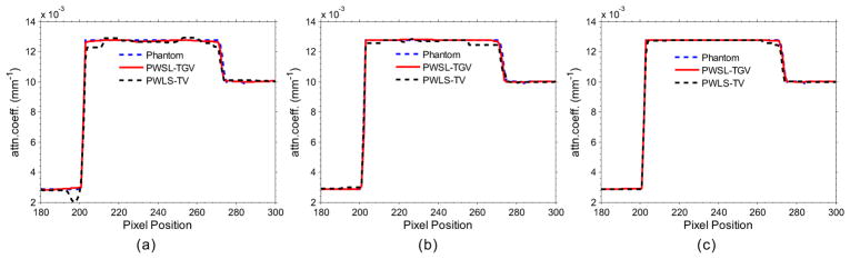
Vertical profiles (296^th column) of the images reconstructed by the PWLS-TV and PWLS-TGV methods from different projections: (a) 30-view projection; (b) 40-view projection; (c) 60-view projection.

Table 1.

Lin’s concordance correlation (CC) coefficient between the profiles from the ideal phantom and those from the image reconstructed by the PWLS-TV and PWLS-TGV methods.

Views	Methods	Sample size	Lin’s CC coefficient	95% confidence interval	p-value
30-view	PWLS-TV	121	0.9964	(0.9948, 0.9974)	p < 0.0001
	PWLS-TGV	121	0.9985	(0.9979, 0.9990)	p < 0.0001
40-view	PWLS-TV	121	0.9987	(0.9981, 0.9991)	p < 0.0001
	PWLS-TGV	121	0.9991	(0.9988, 0.9994)	p < 0.0001
60-view	PWLS-TV	121	0.9992	(0.9988, 0.9994)	p < 0.0001
	PWLS-TGV	121	0.9994	(0.9991, 0.9995)	p < 0.0001

3.1.3. UQI study

To perform the quantitative analysis of the PWLS-TGV method, we studied the UQI, which measures the similarity between reconstructed and true images. The ROI, as indicated by a red rectangular window in figure 1(a), was selected for the calculation of the UQI values. The curves of the UQI values versus the number of projection views for the XCAT phantom are shown in figure 5. The PWLS-TGV method has higher UQI values than the PWLS-TV method, especially in the 30- and 40- view projection.

Figure 5.

The curves of UQI values versus the number of projection views (a), and the zoomed curves from the 30-view projection to the 116-view projection (b).

3.1.4. MTF measure

Figure 6 shows the MTFs obtained by the PWLS-TGV and PWLS-TV methods for the 30-, 40- and 60- view projection. We can observe that the PWLS-TGV method can yield a better image resolution than the PWLS-TV method in all cases.

Figure 6.

MTF curves from the PWLS-TGV and PWLS-TV methods in three cases: (a) 60-view projection; (b) 40-view projection; (c) 30-view projection.

3.2. Anthropomorphic torso phantom study

3.2.1. Visualization-based evaluation

Figures 7 and 8 show the images reconstructed by the different methods at 100 and 40 mAs. To further display the gains of the PWLS-TGV method, the zoomed ROIs (as indicated by the squares in figure 1(c)) are shown in figures 9 and 10. Serious artifacts existed in the FBP results in all cases, and the PWLS-TGV method yielded more noticeable gains than the PWLS-TV method in terms of patchy artifact suppression. To further visualize the difference between the TV- and TGV-based approaches, vertical profiles of the resulting images (figures 11 and 12) were drawn across the 67^th column, that is, from the 236^th row to the 263^th row. The results suggest that compared with the PWLS-TV method, the PWLS-TGV method can achieve better profiles that match the gold standard.

Figure 7.

Images reconstructed by the FBP, PWLS-TV, and PWLS-TGV methods from 58-, 116-, 232-, 290-, 387-, 580-, and 1160- view projection at 100 mAs.

Figure 8.

Images reconstructed by the FBP, PWLS-TV, and PWLS-TGV methods from 58-, 116-, 232-, 290-, 387-, 580-, and 1160- view projection at 40 mAs.

Figure 9.

Zoomed-in views of images reconstructed by the FBP (1^th row), PWLS-TV (2^th row), and PWLS-TGV (3^th row) methods from 58-, 116-, 232-, 290-, 387-, 580-, and 1160-view projection at 100 mAs.

Figure 10.

Zoomed-in views of images reconstructed by the FBP (1^th row), PWLS-TV (2^th row), and PWLS-TGV (3^th row) methods from 58-, 116-, 232-, 290-, 387-, 580-, and 1160-view projection at 40 mAs.

Figure 11.

Vertical profiles (67^th column) of the images reconstructed by the PWLS-TV and PWLS-TGV methods from different projections at 100 mAs: (a) 58-view projection; (b) 116-view projection; (c) 232-view projection; (d) 290-view projection; (e) 387-view projection; (f) 580-view projection.

Figure 12.

Vertical profiles (67^th column) of the images reconstructed by the PWLS-TV and PWLS-TGV methods from different projections at 40 mAs: (a) 58-view projection; (b) 116-view projection; (c) 232-view projection; (d) 290-view projection; (e) 387-view projection; (f) 580-view projection.

3.2.2. Normal vector flow study

To further verify the improvement of the PWLS-TGV method over the PWLS-TV method, small ROI from the results of the 232-view projection were selected and used in the plotting of the normal vector flow (NVF) images (figures 13 and 14) at 100 and 40 mAs. The NVF image of the FBP reconstruction based on the averaged full-view (1160-view) sinogram data of the scans repeated 150 times was drawn as gold standard. The gradual changes in the intensities of the desired image are often shown as ordered arrows in NVF images, whereas the noise in the image is often shown as disordered arrows, as shown in figures 13(b) and 14(c). The NVF image of the PWLS-TGV method illustrates the recovery of a large number of ordered arrows. This condition indicates the good preservation of the small textures of the resulting image, as indicated by the circles in figures 13(d) and 14(c).

Figure 13.

NVF images of the reconstructed images by the PWLS-TV, and PWLS-TGV methods from 232-view projection at 100 mAs: (a) from the FBP with 1160-view (the gold standard); (b) from the FBP; (c) from the PWLS-TV method; and (d) from the PWLS-TGV method.

Figure 14.

NVF images of the reconstructed images by different methods from 232-view projection at 40 mAs: (a) from the FBP; (b) from the PWLS-TV method; and (c) from the PWLS-TGV method.

3.2.3. UQI study

In the UQI evaluation, the gold standard image (figure 1(c)) was reconstructed by the FBP method with ramp filter at full view based on the averaged sinogram data with scans repeated 150 times and at 100 mAs and 120 kVp. Figure 15 shows the curves of the UQI values versus the number of projection views. The PWLS-TGV results have a higher UQI value than the PWLS-TV results. Thus, the PWLS-TV method can produce more closely matching results compared with the PWLS-TV method in the sparse-view case.

Figure 15.

Curves of the UQI values versus the number of projection views from the PWLS-TV and PWLS-TGV methods: (a) 100 mAs; (b) 40 mAs.

4. Discussion

TV-based methods have been widely used in CT image reconstruction based on noisy and/or sparse-view projection measurements with noticeable gains compared with other existing methods. For example, the PWLS-TV method outperforms the quadratic regularization-based PWLS method based on sparse-view projection measurements in terms of streak artifact suppression (Tang et al, 2009, Liu et al, 2013). However, one major drawback of TV-based methods is that the associative results often suffer from patchy artifacts because of the PCA of the TV model (Tang et al, 2009, Liu et al, 2013).

To eliminate the drawback of the original TV-based methods in sparse-view CT image reconstruction, we introduced the TGV model under the PWLS criteria, which considers the first and second derivatives of an image. The effectiveness of the present PWLS-TGV method in sparse-view CT image reconstruction was extensively validated and evaluated in terms of accuracy and resolution properties in section of Results. The PWLS-TGV method can yield satisfactory results at uniform regions with patchy artifact elimination and around the edges with detailed information preservation. The MTF and UQI studies indicate the superiority of the gains from the PWLS-TGV method over those from the PWLS-TV method in terms of the quantitative measurement of image quality. As shown in the studies on the digital XCAT phantom, the proposed method demonstrates impressive performance with regard to quantitative measure and visual inspection. However, in realistic CT imaging, projection data are affected by photon count noise and electrical background noise. Many reconstruction methods have therefore failed to demonstrate their gains in a realistic scanning environment. Hence, we further validated the proposed method in two different scenarios (i.e., normal- and low-dose cases) using physical phantom imaging. In both cases, the PWLS-TGV method outperformed the PWLS-TV method in sparse-view CT image reconstruction in terms of visual inspection and UQI measure. In other words, the present PWLS-TGV method is more suitable than the PWLS-TV method in a realistic scanning environment.

As indicated by the studies on the XCAT phantom, the present algorithm can monotonically converge to a steady solution in terms of rRMSE measure (figure 2). To yield a convergence result, several parameters should be optimally selected. Such requirement is an open problem for all the regularized iterative CT image reconstruction methods (Wang et al, 2011). For the present PWLS-TGV method, six parameters need to be determined, i.e., β₁, β₂, ρ, τ, α₀, and α₁. As β₁ mainly depends on the intensities of the desired image during implementation, it can be optimally selected before running the algorithm. ρ and τ as step variables can be optimized according to the scheme introduced in a previous study (Knoll et al, 2011). β₂ as a hyper-parameter controls the smoothness of the reconstructed image, which can be determined by a broader range of parameter values in terms of rRMSE and eye-appealing visualization compared with the gold standard. For compatibility with the usual TV regularization, α₁ = 1 and α₀ = 3 were used in all the applications throughout the current study. Similar to most SIR methods in CT image reconstruction (Ma et al, 2012a, Lauzier Thériault and Chen, 2013), the computational cost of the present PWLS-TGV method is very large because of the projection and back-projection operations using a huge system matrix. However, with the development of fast computers and dedicated hardware (Xu and Mueller, 2005, Knaup et al, 2006), iterative reconstruction algorithms, including the present PWLS-TGV method, may be used in clinical CT reconstruction in the near future.

The PWLS-TGV method presented in the current work was only focused on CT image reconstruction based on sparse-view projections. The present method can also be used in other X-ray CT applications, including limited angle reconstruction (Persson et al, 2001, Sidky et al, 2006) and interior tomography (Yu and Wang, 2009). In addition, the PWLS-TVG method can be efficiently applied in regularizing many types of inverse problems in tomographic imaging, such as phase-contrast CT (Ma et al, 2010), and SPECT (Wolf et al, 2013). This feature is an interesting topic for future research.

5. Conclusion

With the goal of reducing the radiation dose in CT image examinations, we proposed the PWLS-TGV method, which is a TGV regularization model under the PWLS criteria for CT image reconstruction based on sparse-view projection measurements. The use of the proposed PWLS-TGV method is aimed at relieving the piecewise constant assumption of TV-based methods for sparse-view CT image reconstruction. The proposed PWLS-TGV method can achieve significant gains compared with the PWLS-TV method in terms of the preservation of structural details and the suppression of image noise as well as undesired patchy artifacts. In other words, the proposed PWLS-TGV method has useful potential for radiation dose reduction by lowering the mAs and reducing the number of projection views.

References

- Bian J, Siewerdsen J, Han X, Sidky E, Prince J, Pelizzari C, Pan X. Evaluation of sparse-view reconstruction from flat-panel-detector cone-beam CT. Phys Med Biol. 2010;55:6575–99. doi: 10.1088/0031-9155/55/22/001. [DOI] [PMC free article] [PubMed] [Google Scholar]
- Bian Z, Ma J, Huang J, Zhang H, Niu S, Feng Q, Liang Z, Chen W. SR-NLM: A sinogram restoration induced non-local means image filtering for low-dose computed tomography. Comput Med Imaging Graph. 2013;37:293–303. doi: 10.1016/j.compmedimag.2013.05.004. [DOI] [PMC free article] [PubMed] [Google Scholar]
- Bredies K, Valkonen K. Inverse problems with second-order total generalized variation constraints. Proceedings of SampTA. 2011 ( http://www.uni-graz.at/~bredies/papers/SampTA2011.pdf)
- Bredies K, Kunisch K, Pock T. Total generalized variation. SIAM J Imaging Sci. 2010;3:492–526. [Google Scholar]
- Bredies K, Dong Y, Hintermüller M. Spatially dependent regularization parameter selection in total generalized variation models for image restoration. Int J Comput Math. 2013;90:109–23. [Google Scholar]
- Chambolle A, Pock T. A first-order primal-dual algorithm for convex problems with applications to imaging. J Math Imaging Vis. 2011;40:120–45. [Google Scholar]
- Chen G, Tang J, Leng S. Prior image constrained compressed sensing (PICCS): a method to accurately reconstruct dynamic CT images from highly under sampled projection data sets. Med Phys. 2008;35:660–3. doi: 10.1118/1.2836423. [DOI] [PMC free article] [PubMed] [Google Scholar]
- Chen Z, Jin X, Li L, Wang G. A limited-angle CT reconstruction method based on anisotropic TV minimization. Phys Med Biol. 2013;58:2119–41. doi: 10.1088/0031-9155/58/7/2119. [DOI] [PubMed] [Google Scholar]
- Einstein A, Henzlova M, Rajagopalan S. Estimating risk of cancer associated with radiation exposure from 64-slice CT coronary angiography. J Am Med Assoc. 2007;298:317–23. doi: 10.1001/jama.298.3.317. [DOI] [PubMed] [Google Scholar]
- Elbakri I, Fessler J. Statistical image reconstruction for polyenergetic X-ray computed tomography. IEEE Trans Med Imaging. 2002;21:89–99. doi: 10.1109/42.993128. [DOI] [PubMed] [Google Scholar]
- Fahimian B, Mao Y, Cloetens P, Miao J. Low-dose X-ray phase-contrast and absorption CT using equally sloped tomography. Phys Med Biol. 2010;55:5383–400. doi: 10.1088/0031-9155/55/18/008. [DOI] [PubMed] [Google Scholar]
- Han X, Bian J, Ritman E, Sidky E, Pan X. Optimization based reconstruction of sparse images from few-view projections. Phys Med Biol. 2012;57:5245–73. doi: 10.1088/0031-9155/57/16/5245. [DOI] [PMC free article] [PubMed] [Google Scholar]
- Huang J, Zhang Y, Ma J, Zeng D, Bian Z, Niu S, Feng Q, Liang Z, Chen W. Iterative image reconstruction for sparse-view CT using normal-dose image induced total variation prior. PLOS ONE. 2013;8:e79709. doi: 10.1371/journal.pone.0079709. [DOI] [PMC free article] [PubMed] [Google Scholar]
- Huang Y, Ng M, Wen Y. A fast total variation minimization method for image restoration. SIAM Multiscale Model Simul. 2008;7:774–95. [Google Scholar]
- Jorgensen J, Sidky E, Pan X. Quantifying admissible undersampling for sparsity-exploiting iterative image reconstruction in X-ray CT. IEEE Trans Med Imaging. 2013;32:460–73. doi: 10.1109/TMI.2012.2230185. [DOI] [PMC free article] [PubMed] [Google Scholar]
- Kalra M, Maher M, Toth T, Schmidt B, Westerman B, Morgan H, Saini S. Techniques and applications of automatic tube current modulation for CT. Radiology. 2004;233:649–57. doi: 10.1148/radiol.2333031150. [DOI] [PubMed] [Google Scholar]
- La Riviére P, Bian J, Vargas P. Penalized-likelihood sinogram restoration for computed tomography. IEEE Trans Med Imaging. 2006;25:1022–36. doi: 10.1109/tmi.2006.875429. [DOI] [PubMed] [Google Scholar]
- Lauzier Thériault P, Tang J, Chen G. Prior image constrained compressed sensing: Implementation and performance evaluation. Med Phys. 2012;39:66–80. doi: 10.1118/1.3666946. [DOI] [PMC free article] [PubMed] [Google Scholar]
- Lauzier Thériault P, Chen G. Characterization of statistical prior image constrained compressed sensing (PICCS): II. Application to dose reduction. Med Phys. 2013;40:021902. doi: 10.1118/1.4773866. [DOI] [PMC free article] [PubMed] [Google Scholar]
- Lewis R. Medical phase contrast X-ray imaging: current status and future prospects. Phys Med Biol. 2004;49:3573–83. doi: 10.1088/0031-9155/49/16/005. [DOI] [PubMed] [Google Scholar]
- Li T, Li X, Wang J, Wen J, Lu H, Hsieh J, Liang Z. Nonlinear sinogram smoothing for low-dose X-ray CT. IEEE Trans Nucl Sci. 2004;51:2505–13. [Google Scholar]
- Liu Y, Ma J, Fan Y, Liang Z. Adaptive-weighted total variation minimization for sparse data toward low-dose X-ray computed tomography image reconstruction. Phys Med Biol. 2012;57:7923–56. doi: 10.1088/0031-9155/57/23/7923. [DOI] [PMC free article] [PubMed] [Google Scholar]
- Liu Y, Liang Z, Ma J, Lu H, Wang K, Zhang H, Moore W. Total variation-stokes strategy for sparse-view X-ray CT image reconstruction. IEEE Trans Med Imaging. 2014;33:749–63. doi: 10.1109/TMI.2013.2295738. [DOI] [PMC free article] [PubMed] [Google Scholar]
- Ma J, Feng Q, Feng Y, Huang J, Chen W. Generalized Gibbs priors based positron emission tomography reconstruction. Comput Biol Med. 2010;40:565–71. doi: 10.1016/j.compbiomed.2010.03.012. [DOI] [PubMed] [Google Scholar]
- Ma J, Huang J, Feng Q, Zhang H, Lu H, Liang Z, Chen W. Low-dose computed tomography image restoration using previous normal-dose scan. Med Phys. 2011;38:5713–31. doi: 10.1118/1.3638125. [DOI] [PMC free article] [PubMed] [Google Scholar]
- Ma J, Zhang H, Gao Y, Huang J, Liang Z, Feng Q, Chen W. Iterative image reconstruction for cerebral perfusion CT using pre-contrast scan induced edge-preserving prior. Phys Med Biol. 2012a;57:7519–42. doi: 10.1088/0031-9155/57/22/7519. [DOI] [PMC free article] [PubMed] [Google Scholar]
- Ma J, Liang Z, Fan Y, Liu Y, Huang J, Chen W, Lu H. Variance analysis of X-ray CT sinograms in the presence of electronic noise background. Med Phys. 2012b;39:4051–65. doi: 10.1118/1.4722751. [DOI] [PMC free article] [PubMed] [Google Scholar]
- McCollough C, Bruesewitz M, Kofler J., Jr CT dose reduction and dose management tools: overview of available options. Radiographics. 2006;26:503–12. doi: 10.1148/rg.262055138. [DOI] [PubMed] [Google Scholar]
- Niu T, Zhu L. Accelerated barrier optimization compressed sensing (ABOCS) reconstruction for cone-beam CT: Phantom studies. Med Phys. 2012;39:4588–98. doi: 10.1118/1.4729837. [DOI] [PMC free article] [PubMed] [Google Scholar]
- Panin V, Zeng G, Gullberg G. Total variation regulated EM algorithm. IEEE Trans Nucl Sci. 1999;46:2202–10. [Google Scholar]
- Park J, Song B, Kim J, Park S, Kim H, Liu Z, Suh T, Song W. Fast compressed sensing-based CBCT reconstruction using Barzilai-Borwein formulation for application to on-line IGRT. Med Phys. 2012;39:1207–17. doi: 10.1118/1.3679865. [DOI] [PubMed] [Google Scholar]
- Persson M, Bone D, Elmqvist H. Total variation norm for three-dimensional iterative reconstruction in limited view angle tomography. Phys Med Biol. 2001;46:853–66. doi: 10.1088/0031-9155/46/3/318. [DOI] [PubMed] [Google Scholar]
- Rudin L, Osher S, Fatemi E. Nonlinear total variation based noise removal algorithms. Phys D. 1992;60:259–68. [Google Scholar]
- Segars W, Sturgeon G, Mendonca S, Grimes J, Tsui B. 4D XCAT phantom for multimodality imaging research. Med Phys. 2010;37:4902–15. doi: 10.1118/1.3480985. [DOI] [PMC free article] [PubMed] [Google Scholar]
- Sidky E, Kao C, Pan X. Accurate image reconstruction from few-views and limited-angle data in divergent-beam CT. J X-ray Sci Technol. 2006;14:119–39. [Google Scholar]
- Sidky E, Pan X. Image reconstruction in circular cone-beam computed tomography by constrained, total-variation minimization. Phys Med Biol. 2008;53:4777–807. doi: 10.1088/0031-9155/53/17/021. [DOI] [PMC free article] [PubMed] [Google Scholar]
- Tang J, Nett B, Chen G. Performance comparison between total variation (TV)-based compressed sensing and statistical iterative reconstruction algorithms. Phys Med Biol. 2009;54:5781–804. doi: 10.1088/0031-9155/54/19/008. [DOI] [PMC free article] [PubMed] [Google Scholar]
- Tian Z, Jia X, Yuan K, Pan T, Jiang S. Low-dose CT reconstruction via edge-preserving total variation regularization. Phys Med Biol. 2011;56:5949–67. doi: 10.1088/0031-9155/56/18/011. [DOI] [PMC free article] [PubMed] [Google Scholar]
- Wang Z, Bovik A. A universal image quality index. IEEE Signal Proc Let. 2002;9:81–4. [Google Scholar]
- Wang J, Guan H, Solberg T. Inverse determination of the penalty parameter in penalized weighted least-squares algorithm for noise reduction of low-dose CBCT. Med Phys. 2011;38:4066–72. doi: 10.1118/1.3600696. [DOI] [PubMed] [Google Scholar]
- Wang J, Li T, Lu H, Liang Z. Penalized weighted least-squares approach to sinogram noise reduction and image reconstruction for low-dose X-ray computed tomography. IEEE Trans Med Imaging. 2006;24:1272–83. doi: 10.1109/42.896783. [DOI] [PMC free article] [PubMed] [Google Scholar]
- Wang J, Liang Z, Lu H, Lei X. Recent development of low-dose X-ray cone-beam computed tomography. Curr Med Imaging Rev. 2010;6:72–81. [Google Scholar]
- Wang J, Lu H, Liang Z, Eremina D, Zhang G, Wang S, Chen J, Manzione J. An experimental study on the noise properties of X-ray CT sinogram data in Radon space. Phys Med Biol. 2008;53:3327–41. doi: 10.1088/0031-9155/53/12/018. [DOI] [PMC free article] [PubMed] [Google Scholar]
- Wang J, Li T, Xing L. Iterative image reconstruction for CBCT using edge-preserving prior. Med Phys. 2009;36:252–60. doi: 10.1118/1.3036112. [DOI] [PMC free article] [PubMed] [Google Scholar]
- Wang G, Yu H. The meaning of interior tomography. Phys Med Biol. 2004;58:R161–86. doi: 10.1088/0031-9155/58/16/R161. [DOI] [PMC free article] [PubMed] [Google Scholar]
- Wolf P, Jørgensen J, Schmidt T, Sidky E. Few-view single photon emission computed tomography (SPECT) reconstruction based on a blurred piecewise constant object model. Phys Med Biol. 2013;58:5629–52. doi: 10.1088/0031-9155/58/16/5629. [DOI] [PMC free article] [PubMed] [Google Scholar]
- Xu F, Mueller K. Accelerating popular tomographic reconstruction algorithms on commodity PC graphics hardware. IEEE Trans Nucl Sci. 2005;52:654–63. [Google Scholar]
- Xu Q, Yu H, Mou X, Zhang L, Hsieh J, Wang G. Low-dose X-ray CT reconstruction via dictionary learning. IEEE Trans Med Imaging. 2012;31:1682–97. doi: 10.1109/TMI.2012.2195669. [DOI] [PMC free article] [PubMed] [Google Scholar]
- Yu L, Bruesewitz M, Thomas K, Fletcher J, Kofler J, McCollough C. Optimal tube potential for radiation dose reduction in pediatric CT: principles, clinical implementations, and pitfalls. Radiographics. 2011;31:835–48. doi: 10.1148/rg.313105079. [DOI] [PubMed] [Google Scholar]
- Yu D, Fessler J. Edge-preserving tomographic reconstruction with nonlocal regularization. IEEE Trans Med Imaging. 2002;21:159–73. doi: 10.1109/42.993134. [DOI] [PubMed] [Google Scholar]
- Yu H, Wang G. Compressed sensing based interior tomography. Phys Med Biol. 2009;54:2791–805. doi: 10.1088/0031-9155/54/9/014. [DOI] [PMC free article] [PubMed] [Google Scholar]