Bayesian Semiparametric Density Deconvolution in the Presence of Conditionally Heteroscedastic Measurement Errors

Abstract

We consider the problem of estimating the density of a random variable when precise measurements on the variable are not available, but replicated proxies contaminated with measurement error are available for sufficiently many subjects. Under the assumption of additive measurement errors this reduces to a problem of deconvolution of densities. Deconvolution methods often make restrictive and unrealistic assumptions about the density of interest and the distribution of measurement errors, e.g., normality and homoscedasticity and thus independence from the variable of interest. This article relaxes these assumptions and introduces novel Bayesian semiparametric methodology based on Dirichlet process mixture models for robust deconvolution of densities in the presence of conditionally heteroscedastic measurement errors. In particular, the models can adapt to asymmetry, heavy tails and multimodality. In simulation experiments, we show that our methods vastly outperform a recent Bayesian approach based on estimating the densities via mixtures of splines. We apply our methods to data from nutritional epidemiology. Even in the special case when the measurement errors are homoscedastic, our methodology is novel and dominates other methods that have been proposed previously. Additional simulation results, instructions on getting access to the data set and R programs implementing our methods are included as part of online supplemental materials.

1 Introduction

Many problems of practical importance require estimation of the unknown density of a random variable. The variable, however, may not be observed precisely, observations being subject to measurement errors. Under the assumption of additive measurement errors, the observations are generated from a convolution of the density of interest and the density of the measurement errors. The problem of estimating the density of interest from available contaminated measurements then becomes a problem of deconvolution of densities.

This article proposes novel Bayesian semiparametric approaches for robust estimation of the density of interest when the variability of the measurement errors depends on the associated unobserved value of the variable of interest through an unknown relationship. The proposed methodology is fundamentally different from existing deconvolution methods, relaxes many restrictive assumptions of existing approaches by allowing both the density of interest and the distribution of measurement errors to deviate from standard parametric laws, and significantly outperforms previous methodology.

The literature on the problem of density deconvolution is vast. Most of the early literature on density deconvolution considers scenarios when a single contaminated measurement is available for each subject and assumes that the measurement errors are independently and identically distributed according to some known probability law (often normal) with constant variance. See, for example, Carroll and Hall (1988), Liu and Taylor (1989), Devroye (1989), Fan (1991a, 1991b, 1992) and Hesse (1998) among others. Of course, in reality the distribution of measurement errors is rarely known, and the assumption of constant variance measurement errors is also often unrealistic. The difficulty of a deconvolution problem depends directly on the shape (more specifically the smoothness) of the measurement error distribution (Fan 1991a, 1991b, 1992). Misspecification of the distribution of measurement errors may therefore lead to biased and inefficient estimates of the density of interest. The focus of recent deconvolution literature has thus been on robust deconvolution methods that relax the restrictive assumptions on the error distribution, assuming the availability of replicated proxies for each unknown value of the variable of interest. See, for example, Li and Vuong (1998) and Carroll and Hall (2004) among others.

All the above mentioned papers still assume that the measurement errors are independent of the variable of interest. Staudenmayer, et al. (2008) further relaxed this often unrealistic assumption and considered the problem of density deconvolution in the presence of conditionally heteroscedastic measurement errors. They took a Bayesian route and modeled the density of interest by a penalized positive mixture of normalized quadratic B-splines. Measurement errors were assumed to be normally distributed but the measurement error variance was modeled as a function of the associated unknown value of the variable of interest using a penalized positive mixture of quadratic B-splines.

The focus of this article is also on deconvolution in the presence of conditionally heteroscedastic measurement errors, but the proposed Bayesian semiparametric methods are vastly different from the approach of Staudenmayer, et al. (2008), as well as from other existing methods. The density of interest is modeled by a flexible location-scale mixture of normals induced by a Dirichlet process (Ferguson, 1973; Lo, 1984). For modeling conditionally heteroscedastic measurement errors, it is assumed that the measurement errors can be factored into ‘scaled errors’ that are independent of the variable of interest and have zero mean and unit variance, and a ‘variance function’ component that explains the conditional heteroscedasticity. This multiplicative structural assumption on the measurement errors was implicit in Staudenmayer, et al. (2008), where the scaled errors were assumed to come from a standard normal distribution.

Our approach is based on a more flexible representation of the scaled errors. The density of the scaled measurement errors is modeled using an infinite mixture model induced by a Dirichlet process, each component of the mixture being itself a two-component normal mixture with mean zero. This gives us the flexibility to model other aspects of the distribution of scaled errors. This deconvolution approach, therefore, uses flexible Dirichlet process mixture models twice, first to model the density of interest and second to model the density of the scaled errors, freeing them both from restrictive parametric assumptions, while at the same time accommodating conditional heteroscedasticity through the variance function.

It is important to see that even when the measurement errors are homoscedastic, our methodology is novel and dominates other methods that have been proposed previously. Our methods apply to this problem, allowing flexibility in the density of the variable of interest, flexible representations of the density of the measurement errors, and, if desired, at the same time build modeling robustness lest there be any remaining heteroscedasticity.

The article is organized as follows. Section 2 details the models. Sections 3 discusses some model diagnostic tools. Section 4 presents extensive simulation studies comparing the proposed semiparametric methods with the method of Staudenmayer, et al. (2008) and a possible nonparametric alternative. Section 5 presents an application of the proposed methodology in estimation of the distributions of daily dietary intakes from contaminated 24 hour recalls in a nutritional epidemiologic study. Section 6 contains concluding remarks. Appendices discuss model identifiability (Appendix A), the choice of hyper-parameters (Appendix B) and details of posterior computations (Appendix C). The supplementary materials provide results of additional simulation experiments and R programs implementing our methods.

2 Density Deconvolution Models

2.1 Background

The goal is to estimate the unknown density of a random variable X. There are i = 1, 2, …, n subjects. Precise measurements of X are not available. Instead, for j = 1, 2, …, m_i, replicated proxies W_ij contaminated with heteroscedastic measurement errors U_ij are available for each subject. The replicates are assumed to be generated by the model

$$W_{ij}=X_i+U_{ij},$$ (1)

$$U_{ij}=v^{1/2}(X_i){\epsilon }_{ij},$$ (2)

where X_i is the unobserved true value of X; ε_ij are independently and identically distributed with zero mean and unit variance and are independent of the X_i, and v is an unknown smooth variance function. Identifiability of model (1)–(2) is discussed in Appendix A, where we show that 3 replicates more than suffices. Some simple diagnostic tools that may be employed in practical applications to assess the validity of the structural assumption (2) on the measurement errors are discussed in Section 3.

Of course, a special case of our work is when the measurement errors are homoscedastic, so that v(x) is constant. Even in this case, the use of Dirichlet process mixtures for both the target density and error distribution has not been considered previously.

The density of X is denoted by f_X. The density of ε_ij is denoted by f_ε. The implied conditional distributions of W_ij and U_ij, given X_i, is denoted by the generic notation f_W|X and f_U|X, respectively. The marginal density of W_ij is denoted by f_W.

Model (2), along with the moment restrictions imposed on the scaled errors ε_ij, implies that the conditional heteroscedasticity of the measurement errors is explained completely through the variance function v, while other features of f_U|X are derived from f_ε. In a Bayesian hierarchical framework, model (1)–(2) reduces the problem of deconvolution to three separate problems: (a) modeling the density of interest f_X; (b) modeling the variance function v, and (c) modeling the density of the scaled errors f_ε.

2.2 Modeling the Distribution of X

We use Dirichlet process mixture models (DPMMs) (Ferguson, 1973, Escobar and West, 1995) for modeling f_X. For modeling a density f, a DPMM with concentration parameter α, base measure P₀, and mixture components coming from a parametric family {f_c(· | ϕ): ϕ ~ P₀}, can be specified as

$$f(·)={\sum }_{k=1}^{\infty }{\pi }_k{f}_c(·\mid {\mathit{\varphi }}_k),{\mathit{\varphi }}_k~P_0,{\pi }_k=s_k{\prod }_{j=1}^{k-1}(1-s_j),s_k~\text{Beta}(1,\alpha ).$$

In the literature, this construction of random mixture weights ${\{{\pi }_k\}}_{k=1}^{\infty }$ (Sethuraman, 1994), is often represented as π ~ Stick(α). DPMMs are, therefore, mixture models with a potentially infinite number of mixture components or ‘clusters’. For a given data set of finite size, however, the number of active clusters exhibited by the data is finite and can be inferred from the data.

Choice of the parametric family {f_c(· | ϕ): ϕ ~ P₀} is important. Mixtures of normal kernels are, in particular, very popular for their flexibility and computational tractability (Escobar and West, 1995; West, et al. 1994). In this article also, f_X is specified as a mixture of normal kernels, with a conjugate normal-inverse-gamma (NIG) prior on the location and scale parameters

$$f_X(X)={\sum }_{k=1}^{\infty }{\pi }_k\text{Normal}(X\mid {\mu }_k,{\sigma }_k^2),$$ (3)

$$\pi ~\text{Stick}({\alpha }_X),({\mu }_k,{\sigma }_k^2)~\text{NIG}({\mu }_0,{\sigma }_0^2/{\nu }_0,{\gamma }_0,{\sigma }_0^2).$$ (4)

Here Normal(· | μ, σ²) denotes a normal distribution with mean μ and standard deviation σ. In what follows, the generic notation p₀ will sometimes be used for specifying priors and hyper-priors.

2.3 Modeling the Variance Function

Examples of modeling log-transformed variance functions using flexible mixtures of splines are abundant in the literature when there is no measurement error. Yau and Kohn (2003), for example, modeled log{v(X)} using flexible mixtures of polynomial and thin-plate splines. Liu, et al. (2006) proposed a penalized mixture of smoothing splines, whereas Chan, et al. (2006) considered mixtures of locally adaptive radial basis functions.

In this article we model the variance function as a positive mixture of B-spline basis functions with smoothness inducing priors on the coefficients. For a given positive integer K, partition an interval [A, B] of interest into K subintervals using knot points t₁ = ··· = t_q+1 = A < t_q+2 < t_q+3 < ··· < t_q+K < t_q+K+1 = ··· = t_2q+K+1 = B. For j = (q +1), …, (q + K), define Δ_j = (t_j+1 − t_j) and Δ_max = max_j Δ_j. It is assumed that Δ_max → 0 as K → ∞. Using these knot points, (q + K) = J B-spline bases of degree q, denoted by B_q,J = {b_q,1, b_q,2, …, b_q,J}, can be defined through the recursion relation given on page 90 of de Boor (2000), see Figure S.1 in the supplementary materials. A flexible model for the variance function is

$$v(X)={\sum }_{j=1}^J{b}_{q,j}(X)exp({\xi }_j)={\mathbf{B}}_{q,J}(X)exp(\mathit{\xi }),$$ (5)

$$p_0(\mathit{\xi }\mid J,{\sigma }_{\xi }^2)={\text{MVN}}_J(\mathbf{0},{\sigma }_{\xi }^{-2}P),p_0({\sigma }_{\xi }^2)=\text{IG}(a_{\xi },b_{\xi }).$$ (6)

Here ξ = {ξ₁, ξ₂, …, ξ_J}^T; exp(ξ) = {exp(xi;₁), exp(xi;₂), …, exp(xi;_J)}^T, MVN_J(μ, Σ) denotes a J-variate normal distribution with mean μ and positive semidefinite covariance matrix Σ, and IG(a, b) denotes an inverse-Gamma distribution with shape parameter a and scale parameter b. We choose P = D^TD, where D is a J × (J + 2) matrix such that Dξ computes the second differences in ξ. The prior $p_0(\mathit{\xi }\mid {\sigma }_{\xi }^2)$ induces smoothness in the coefficients because it penalizes ${\sum }_{j=1}^J{({\mathrm{\Delta }}^2{\xi }_j)}^2={\mathit{\xi }}^{\mathrm{T}}P\mathit{\xi }$, the sum of squares of the second order differences in ξ (Eilers and Marx, 1996). The variance parameter ${\sigma }_{\xi }^2$ plays the role of smoothing parameter - the smaller the value of ${\sigma }_{\xi }^2$, the stronger the penalty and the smoother the variance function. The inverse-Gamma hyper-prior on ${\sigma }_{\xi }^2$ allows the data to have strong influence on the posterior smoothness and makes the approach data adaptive.

2.4 Modeling the Distribution of the Scaled Errors

Three different approaches of modeling the density of the scaled errors f_ε are considered here, successively relaxing the model assumptions as we progress.

2.4.1 Model-I: Normal Distribution

We first consider the case where the scaled errors are assumed to follow a standard normal distribution

$$f_{\epsilon }(\epsilon )=\text{Normal}(\epsilon \mid 0,1).$$ (7)

This implies that the conditional density of measurement errors is given by f_U|X(U | X) = Normal{U | 0, v(X)}. Such an assumption was made by Staudenmayer, et al. (2008).

2.4.2 Model-II: Skew-Normal Distribution

The strong parametric assumption of normality of measurement errors may be restrictive and inappropriate for many practical applications. As a first step towards modeling departures from normality, we propose a novel use of skew-normal distributions (Azzalini, 1985) to model the distribution of scaled errors. A random variable Z following a skew-normal distribution with location ξ, scale ω and shape parameter λ has the density f(Z) = (2/ω)ϕ{(Z − xi;)/ω}Φ{λ(Z − ξ)/ω}. Here ϕ and Φ denote the probability density function and cumulative density function of a standard normal distribution, respectively. Positive and negative values of λ result in right and left skewed distributions, respectively. The Normal(· | μ, σ²) distribution is obtained as special cases with λ = 0, whereas the folded normal or half-normal distributions are obtained as limiting cases with λ → ±∞, see Figure S.2 in the supplementary materials. With δ = λ/(1 + λ²)^1/2, the mean and the variance of this density are given by μ = ξ + ωδ(2/π)^1/2 and σ² = ω²(1 − 2δ²/π), respectively. Although the above parametrization is more constructive and intuitive in revealing the relationship with the normal family, we consider a different parametrization in terms of μ, σ² and λ, denoted by SN(· | μ, σ², λ), that is more useful for specifying distributions with moment constraints, namely f(Z) = (2ζ₂/σ)ϕ{ζ₁ + ζ₂(Z − μ)/σ}Φ[λ{ζ₁ + ζ₂(Z − μ)/σ}], where ζ₁ = δ(2/π)^1/2 and ζ₂ = (1 − 2δ²/π)^1/2. For specifying the distribution of the scaled errors we now let

$$f_{\epsilon }(\epsilon )=\text{SN}(\epsilon \mid 0,1,\lambda ),$$ (8)

$$p_0(\lambda )=\text{Normal}(\lambda \mid {\mu }_{0\lambda },{\sigma }_{0\lambda }^2).$$ (9)

The implied conditionally heteroscedastic, unimodal and possibly asymmetric distribution for the measurement errors is given by f_U|X(U | X) = SN{U | 0, v(X), λ}.

2.4.3 Model-III: Infinite Mixture Models

While skew-normal distributions can capture moderate skewness, they are still quite limited in their capacity to model more severe departures from normality. They can not, for example, model multimodality or heavy tails. In the context of regression analysis when there is no measurement error, moment constrained infinite mixture models have recently been used by Pelenis (2014) (see also the references therein) for flexible modeling of error distributions that can capture multimodality and heavy tails. They considered the mixture $f_{U\mid X}(U\mid X)={\sum }_{k=1}^{\infty }{\pi }_k(X)\{p_k\text{Normal}(U\mid {\mu }_{k1},{\sigma }_{k1}^2)+(1-p_k)\text{Normal}(U\mid {\mu }_{k2},{\sigma }_{k2}^2)\}$ , with the moment constraint p_kμ_k1 +(1−p_k)μ_k2 = 0 for all k. Use of a two-component mixture of normals as components with each component constrained to have mean zero restricts the mean of the mixture to be zero while allowing the mixture to model other unconstrained aspects of the error distribution. Incorporating covariate information X in modeling the mixture probabilities, this model allows all aspects of the error distribution, other than the mean, to vary nonparametrically with the covariates, not just the conditional variance. Designed for regression problems, these nonparametric models, however, assume that this covariate information is precise. If X is measured with error, as is the case with deconvolution problems, the subject specific residuals may not be informative enough, particularly when the number of replicates per subject is small and the measurement errors have high conditional variability, making simultaneous learning of X and other parameters of the model difficult.

In this article, we take a different semiparametric middle path. The multiplicative structural assumption (2) on the measurement errors that reduces the problem of modeling f_U|X to the two separate problems of modeling (a) a variance function and (b) modeling an error distribution independent of the variable of interest is retained. The difficult problem of flexible modeling of an error distribution with zero mean and unit variance moment restrictions is avoided through a simple reformulation of model (2) that replaces the unit variance identifiability restriction on the scaled errors by a similar constraint on the variance function. Model (2) is rewritten as

$$U_{ij}=v^{1/2}(X_i){\epsilon }_{ij}=\frac{v^{1/2}(X_i)}{v^{1/2}(X_0)}{v}^{1/2}(X_0){\epsilon }_{ij}={\stackrel{\sim }{v}}^{1/2}(X_i){\stackrel{\sim }{\epsilon }}_{ij},$$ (10)

where X₀ is arbitrary but fixed point, ṽ(X_i) = v(X_i)/v(X₀), and ε̃_ij = v^1/2(X₀)ε_ij. With this specification, ṽ(X₀) = 1, var(ε̃_ij) = v(X₀) and var(U | X) = v(X₀)ṽ(X). The problem of modeling the unrestricted variance function v has now been replaced by the problem of modeling ṽ restricted to have value 1 at X₀. The problem of modeling the density of ε with zero mean and unit variance moment constraints has also been replaced by the easier problem of modeling the density of ε̃_ij with only a single moment constraint of zero mean.

The conditional variance of the measurement errors is now a scalar multiple of ṽ. So ṽ can still be referred to as the ‘variance function’. The variance of ε̃_ij, however, does not equal unity, but is, in fact, unrestricted. With some abuse of nomenclature, ε̃_ij is still referred to as the ‘scaled errors’. For notational convenience ε̃_ij is denoted simply by ε_ij.

The problem of flexibly modeling ṽ is now addressed. For any X, (i) b_q,j(X) ≥ 0 ∀j, (ii) ${\sum }_{j=1}^J{b}_{q,j}(X)=1$, (iii) b_q,j is positive only inside the interval [t_j, t_j+q+1], (iv) for j ∈ {(q + 1), (q+2), …, (q+K)}, for any X ∈ (t_j, t_j+1), only (q+1) B-splines b_q,j−q(X), b_q,j−q+1(X), …, b_q,j(X) are positive, and (v) when X = t_j, b_q,j(X) = 0. We let ṽ(X) = B_q,J (X) exp(ξ), as before, and we use the above mentioned local support properties of the B-spline bases to propose a flexible model for ṽ subject to ṽ(X₀) = 1. When X₀ ∈ (t_j, t_j+1), properties (ii) and (iv) cause the constraint to be simply $\stackrel{\sim }{v}(X_0)={\sum }_{\ell =(q-j)}^j{b}_{q,\ell }(X_0)exp({\xi }_j)=1$. This is a restriction on only (q + 1) of the ξ_j’s, and the coefficients of the remaining B-splines remain unrestricted which makes the model for ṽ very flexible. In a Bayesian framework, the restriction ṽ(X₀) = 1 can be imposed by restricting the support of the prior on ξ to the set { $\mathit{\xi }:{\sum }_{\ell =(q-j)}^j{b}_{q,\ell }(X_0)exp({\xi }_j)=1$}. Choosing X₀ = t_j0 for some j₀ ∈ {(q + 1), …, (q + K)}, we further have b_j0(t_j0) = 0, and the complete model for ṽ is given by

$$\stackrel{\sim }{v}(X)={\mathbf{B}}_{q,J}(X)exp(\mathit{\xi }),$$ (11)

$$p_0(\mathit{\xi }\mid J,{\sigma }_{\xi }^2)={\text{MVN}}_J(\mathbf{0},{\sigma }_{\xi }^{-2}P)\times I\left\{{\sum }_{j=(j_0-q)}^{(j_0-1)}{b}_{q,j}(t_{j0})exp({\xi }_j)=1\right\},$$ (12)

$$p_0({\sigma }_{\xi }^2)=\text{IG}(a_{\xi },b_{\xi }),K~p_0(K),$$ (13)

where I(·) denotes the indicator function.

Now that the variance of ε_ij has become unrestricted and only a single moment constraint of zero mean is required, a DPMM with mixture components as specified in Pelenis (2014) can be used to model f_ε. That is, we let $f_{\epsilon }(\epsilon )={\sum }_{k=1}^{\infty }{\pi }_{\epsilon k}{f}_{c\epsilon }(\epsilon \mid p_k,{\mu }_{k1},{\mu }_{k2},{\sigma }_{k1}^2,{\sigma }_{k2}^2)$, π_ε ~ Stick(α_ε), where $f_{c\epsilon }(\epsilon \mid p,{\mu }_1,{\mu }_2,{\sigma }_1^2,{\sigma }_2^2)=\{p\text{Normal}(\epsilon \mid {\mu }_1,{\sigma }_1^2)+(1-p)\text{Normal}(\epsilon \mid {\mu }_2,{\sigma }_2^2)\}$, subject to the moment constraint pμ₁ + (1 − p)μ₂ = 0. The moment constraint of zero mean implies that each component density can be described by four parameters. One such parametrization that facilitates prior specification is in terms of parameters (p, μ̃, ${\sigma }_1^2,{\sigma }_2^2$), where (μ₁, μ₂) can be retrieved from μ̃ as μ₁ = c₁μ̃, μ₂ = c₂μ̃, where c₁ = (1 − p)/{p² + (1 − p)²}^1/2 and c₂ = −p/{p² + (1 − p)²}^1/2. Clearly the zero mean constraint is satisfied, since pμ₁ + (1 − p) μ₂ = {pc₁ + (1 − p)c₂}μ̃ = 0. The family includes normal densities as special cases with (p, μ̃) = (0.5, 0) or (0, 0) or (1, 0). Symmetric component densities are obtained as special cases when p = 0.5 or μ̃ = 0. The mixture is symmetric when the all components are as well. Specification of the prior for f_ε is completed assuming non-informative priors for (p, μ̃, ${\sigma }_1^2,{\sigma }_2^2$). Letting Unif(ℓ, u) denote a uniform distribution on the interval (ℓ, u), the complete DPMM prior on f_ε can then be specified as

$$f_{\epsilon }(\epsilon )={\sum }_{k=1}^{\infty }{\pi }_{\epsilon k}{f}_{c\epsilon }(\epsilon \mid p_k,{\stackrel{\sim }{\mu }}_k,{\sigma }_{k1}^2,{\sigma }_{k2}^2),$$ (14)

$${\pi }_{\epsilon }~\text{Stick}({\alpha }_{\epsilon }),(p_k,{\stackrel{\sim }{\mu }}_k,{\sigma }_{k1}^2,{\sigma }_{k2}^2)~\text{Unif}(0,1)\text{Normal}(0,{\sigma }_{\stackrel{\sim }{\mu }}^2)\text{IG}(a_{\epsilon },b_{\epsilon })\text{IG}(a_{\epsilon },b_{\epsilon }).$$ (15)

2.5 Choice of Hyper-parameters and Posterior Calculations

Appendix B describes the choice of hyper-parameters, while Appendix C gives the details of posterior computations.

3 Model Diagnostics

In practical deconvolution problems, the basic structural assumptions on the measurement errors may be dictated by prominent features of the data extracted by simple diagnostic tools and expert knowledge of the data generating process. Conditional heteroscedasticity, in particular, is easy to identify from the scatterplot of $S_W^2$ on W̄, where W̄ and $S_W^2$ denote the subject specific sample mean and variance, respectively (Eckert, et al., 1997). The multiplicative structural assumption (2) on the measurement errors provides one particular way of accommodating conditional heteroscedasticity in the model. When at least 4 replicates are available for sufficiently many subjects, one can define the pairs (W_ij1, C_ij2j3j4) for all i and for all j₁ ≠ j₂ ≠ j₃ ≠ j₄, where C_ij2j3j4 = {(W_ij2 − W_ij3)/(W_ij2 − W_ij4)}. When (2) is true, C_j2j3j4= {(ε_j2 − ε_j3)/(ε_j2 − ε_j4)} is independent of W_j1. Therefore, the absence of non-random patterns in the plots of W_j1 against C_j2j3j4 and nonsignificant p-values in nonparametric tests of association between W_j1 and C_j2j3j4 for various j₁ ≠ j₂ ≠ j₃ ≠ j₄ may be taken as indications that (2) is valid or that the departures from (2) are not severe. For those cases with m (≥ 4) replicates per subject, the total number of possible such tests is m!/(m−4)! = L, say, where, for any positive integer r, r! = r ·(r −1) … 2·1. The p-values of these tests can be combined using the truncated product method of Zaykin, et al. (2002). The test statistic of this combined left-sided test is given by $T(\varsigma )={\prod }_{\ell =1}^L{p}_{\ell }^{1(p_{\ell }<\varsigma )}$ , where p_ℓ denotes the p-value of the ℓ^th test and ς is a prespecified truncation limit. If min_ℓ{p_ℓ} ≥ ς, the p-value of the combined test is trivially 1. Otherwise, the bootstrap procedure described in Zaykin, et al. (2002) may be used to estimate it.

4 Simulation Experiments

4.1 Background

The mean integrated squared error (MISE) of estimation of f_X by f̂_X is defined as MISE = ∫ E{f_X(x) − f̂_X(x)}²dx. A Markov chain Monte Carlo (MCMC) algorithm, implemented for drawing samples from the posterior to calculate estimates of f_X and other functions of secondary interest, is detailed in Appendix C. Based on B simulated data sets, a Monte Carlo estimate of MISE is given by ${\mathit{MISE}}_{\mathit{est}}=B^{-1}{\sum }_{b=1}^B{\sum }_{i=1}^N{\{f_X(X_i^{\mathrm{\Delta }})-{\widehat{f}}_X^{(b)}(X_i^{\mathrm{\Delta }})\}}^2{\mathrm{\Delta }}_i$, where ${\{X_i^{\mathrm{\Delta }}\}}_{i=0}^N$ are a set of grid points on the range of X and ${\mathrm{\Delta }}_i=(X_i^{\mathrm{\Delta }}-X_{i-1}^{\mathrm{\Delta }})$ for all i.

The simulation experiments are designed to evaluate the MISE performance of the proposed models for a wide range of possibilities. The Bayesian deconvolution models proposed in this article all take semiparametric routes to model conditional heteroscedasticity assuming a multiplicative structural assumption on the measurement errors. Performance of the proposed models is first evaluated for ‘semiparametric truth scenarios’ when the truth conforms to the assumed multiplicative structure. Efficiency of the proposed models will also be illustrated for ‘nonparametric truth’ scenarios when the truth departs from the assumed multiplicative structure.

The reported estimated MISE are all based on B = 400 simulated data sets. For the proposed methods 5,000 MCMC iterations were run in each case with the initial 3,000 iterations discarded as burn-in. In our R code, with n = 500 subjects and m_i = 3 proxies for each subject, on an ordinary desktop, 5,000 MCMC iterations for models I, II and III required approximately 5 minutes, 10 minutes and 25 minutes, respectively. In comparison, the method of Staudenmayer, et al. (2008) and the nonparametric alternative described below in Section 4.3 took approximately 100 minutes.

4.2 Semiparametric Truth

This subsection presents the results of simulation experiments comparing our methods with the method of Staudenmayer, et al. (2008), referred to as the SRB method. The methods are compared over a factorial combination of three sample sizes (n = 250,500,1000), two densities for $X\{f_X^1(X)=0.5\text{Normal}(X\mid 0,0.75)+0.5\text{Normal}(X\mid 3,0.75)$ and $f_X^2(X)=0.8\text{Normal}(X\mid 0,0.75)+0.2\text{Normal}(X\mid 3,0.75)\}$, nine different types of distributions for the scaled errors (six light-tailed and three heavy-tailed, see Table 1 and Figure 1), and one variance function v(X) = (1 + X/4)². For each subject, m_i = 3 replicates were simulated. The MISE are presented in Table 2. Additional simulation results, where the true f_X is a normalized mixture of B-splines, are presented in the supplementary materials.

Table 1.

The distributions used to generate the scaled errors in the simulation experiment. Let MRTCN(K, π_ε, p, μ̃ ${\mathit{\sigma }}_1^2,{\mathit{\sigma }}_2^2$) denote a K component mixture of moment restricted two-component normals: ${\sum }_{k=1}^K{\pi }_{\epsilon k}{f}_{c\epsilon }(·\mid p_k,{\stackrel{\sim }{\mu }}_k,{\sigma }_{k1}^2,{\sigma }_{k2}^2)$. Then SMRTN denotes a scaled version of MRTCN, scaled to have variance one. Laplace(μ, b) denotes a Laplace distribution with location μ and scale b. SMLaplace(K, π_ε, 0, b) denotes a K component mixture of Laplace densities: ${\sum }_{k=1}^K{\pi }_{\epsilon k}\text{Laplace}(0,b_k)$, scaled to have variance one. With μ_k denoting the k^th order central moments of the scaled errors, the skewness and excess kurtosis of the distribution of scaled errors are measured by the coeficients γ₁ = μ₃ and γ₂ = μ₄ − 3, respectively. The densities (a)–(f) are light-tailed, whereas the densities (g)–(i) are heavy-tailed. The shapes of these distributions are illustrated in Figure 1.

Distribution of scaled errors	Skewness (γ1)	Excess Kurtosis (γ2)
(a) Normal(0,1)	0	0
(b) Skew-normal(0,1,7)	0.917	0.779
(c) SMRTCN(1,1,0.4,2,2,1)	0.499	−0.966
(d) SMRTCN(1,1,0.5,2,1,1)	0	−1.760
(e) SMRTCN{2,(0.3,0.7),(0.6,0.5),(5,0),(1,4),(2,1)}	−0.567	−1.714
(f) SMRTCN{2,(0.3,0.7),(0.6,0.5),(0,4),(0.5,4),(0.5,4)}	0	−1.152
(g) SMRTCN{2,(0.8,0.2),(0.5,0.5),(0,0),(0.25,5),(0.25,5)}	0	7.524
(h) Laplace(0,2−1/2)	0	3
(i) SMLaplace{2,(0.5,0.5),(0,0),(1,4)}	0	7.671

Figure 1.

The distributions used to generate the scaled errors in the simulation experiment, superimposed over a standard normal density. The difierent choices cover a wide range of possibilities - (a) standard normal (not shown separately), (b) asymmetric skew-normal, (c) asymmetric bimodal, (d) symmetric bimodal, (e) asymmetric trimodal, (f) symmetric trimodal, (g) symmetric heavy-tailed, (h) symmetric heavy-tailed with a sharp peak at zero and (i) symmetric heavy-tailed with even a sharper peak at zero. The last six cases demonstrate the flexibility of mixtures of moment restricted two-component normals in capturing widely varying shapes.

Table 2.

Mean integrated squared error (MISE) performance of density deconvolution models described in Section 2 of this article (Models I, II and III) compared with the model of Staudenmayer, et al. (2008) (Model SRB) for different scaled error distributions. The true variance function was v(X) = (1 + X/4)². See Section 4.2 for additional details. The minimum value in each row is highlighted.

True Error Distribution	True X Distribution	Sample Size	MISE × 1000
			SRB	Model1	Model2	Model3
(a)	50–50 mixture of normals	250 500 1000	10.15 6.64 4.50	5.31 3.15 1.96	5.61 3.16 2.08	5.55 3.34 2.21
	80–20 mixture of normals	250 500 1000	9.60 5.30 4.39	4.41 2.34 1.31	4.47 2.39 1.37	4.52 2.62 1.39
(b)	50–50 mixture of normals	250 500 1000	11.79 11.85 8.66	7.80 5.79 4.58	4.41 3.11 1.91	4.55 3.33 2.21
	80–20 mixture of normals	250 500 1000	10.74 7.94 6.16	6.97 4.17 3.08	4.52 2.27 1.26	4.54 2.60 1.39
(c)	50–50 mixture of normals	250 500 1000	12.61 9.27 9.15	8.74 4.91 4.13	5.31 3.57 2.53	4.60 3.39 1.91
	80–20 mixture of normals	250 500 1000	9.27 6.67 5.04	6.46 3.18 2.26	4.65 2.77 1.40	4.03 2.37 1.26
(d)	50–50 mixture of normals	250 500 1000	10.10 6.54 6.02	7.71 4.26 3.41	9.94 7.01 5.58	4.40 2.70 1.40
	80–20 mixture of normals	250 500 1000	8.18 4.45 4.40	5.32 2.67 1.74	5.92 4.30 3.31	3.43 2.21 1.60
(e)	50–50 mixture of normals	250 500 1000	10.03 9.38 8.39	6.01 3.87 2.42	5.92 3.57 2.25	4.03 2.99 1.75
	80–20 mixture of normals	250 500 1000	7.82 7.62 6.82	3.97 3.00 1.74	4.44 2.40 1.45	3.38 2.01 1.17
(f)	50–50 mixture of normals	250 500 1000	9.35 7.18 4.63	5.82 3.47 2.46	6.52 3.67 2.62	5.37 3.62 2.10
	80–20 mixture of normals	250 500 1000	9.17 7.35 3.86	4.75 2.58 1.53	4.80 2.65 1.60	4.10 2.52 1.45
(g)	50–50 mixture of normals	250 500 1000	15.68 23.27 49.77	11.78 15.57 18.91	10.38 14.85 21.00	3.30 2.07 1.12
	80–20 mixture of normals	250 500 1000	20.05 36.46 48.70	8.18 10.83 18.53	15.99 17.23 17.77	3.10 1.63 0.92
(h)	50–50 mixture of normals	250 500 1000	11.29 15.07 18.79	6.62 8.07 12.04	7.01 7.24 8.41	5.18 3.29 1.99
	80–20 mixture of normals	250 500 1000	11.34 13.23 22.03	7.18 7.43 8.64	7.05 7.53 7.56	2.91 1.67 1.03
(i)	50–50 mixture of normals	250 500 1000	19.34 28.79 54.03	7.69 17.32 26.78	9.90 11.02 11.64	3.10 2.14 0.94
	80–20 mixture of normals	250 500 1000	29.81 48.41 57.87	16.45 20.94 23.80	14.76 14.99 16.59	2.74 1.60 0.83

4.2.1 Results for Light-tailed Error Distributions

This section discusses MISE performances of the models for the 36 (3×2×6) cases where the scaled errors were light-tailed, distributions (a)–(f), see Table 1 and Figure 1. Results of the simulation experiments show that all three models proposed in this article significantly out-performed the SRB model in all 36 cases considered. When measurement errors are normally distributed, the reductions in MISE over the SRB method for all three models and for all six possible combination of sample sizes and true X distributions are more than 50%. This is particularly interesting, since the SRB method was originally proposed for normally distributed errors, even more so because our Model-II and Model-III relax the normality assumption on the measurement errors.

4.2.2 Results for Heavy-tailed Error Distributions

This section discusses MISE performances of the models for the 18 (3 × 2 × 3) cases where the distribution of scaled errors were heavy-tailed, distributions (g), (h) and (i), see Table 1 and Figure 1. Results for the error distribution (g) are summarized in Figure 2. The SRB model and Model-I assume normally distributed errors; Model-II assumes skew-normal errors whose tail behavior is similar to that of normal distributions. The results show the MISE performances of these three models to be very poor for heavy-tailed error distributions and the MISE increased with an increase in sample size due to the presence of an increasing number of outliers. Model-III, on the other hand, can accommodate heavy-tails in the error distributions and is, therefore, very robust to the presence of outliers. MISE patterns produced by Model-III for heavy-tailed errors were similar to that for light-tailed errors, and improvements in MISE over the other models were huge. For example, when the density for the scaled was (i), a mixture of Laplace densities with a very sharp peak at zero, for n = 1000, the improvements in MISEs over the SRB model were 54.03/0.94 ≈ 57 times for the 50–50 mixture of normals and 57.87/0.83 ≈ 70 times for the 80–20 mixture of normals.

Figure 2.

Results for heavy-tailed error distribution (g) with sample size n=1000 corresponding to 25^th percentile MISE. The top panel shows the estimated densities under different models. The bottom left panel shows estimated densities of scaled errors under Model-II (dashed line) and Model-III (solid bold line) superimposed over a standard Normal density (solid line). The bottom right panel shows estimated variance functions under different models. For the top panel and the bottom right panel, the solid thin line is for Model-I; the dashed line is for Model-II; the solid bold line is for Model-III; and the dot-dashed line is for the Model of Staudenmayer, et al. (2008). In all three panels the bold gray lines represent the truth.

In simpler settings, when the measurement errors are independent of the variable of interest and have a known density, Fan (1991a, 1991b, 1992) showed that the dificulty of a deconvolution problem depends directly on the shape (more specifically the smoothness) of the measurement error distribution. The results of our simulation experiments provide empirical evidence in favor of a similar conclusion in more complicated and realistic deconvolution scenarios, where the measurement errors show strong patterns of conditional heteroscedasticity, and illustrate the importance of modeling the shape of the error distribution when it is unknown.

4.3 Nonparametric Truth

This subsection is aimed at providing some empirical support to the claim made in Section 2.4.3, where it was argued that for deconvolution problems the proposed semiparametric route to model the distribution of conditionally heteroscedastic measurement errors will often be more efficient than possible nonparametric alternatives, even when the truth departs from the assumed multiplicative structural assumption (2) on the measurement errors. This is done by comparing our Model III with a method that also models the density of interest by a DPMM like ours but employs the formulation of Pelenis (2014) to model the density of the measurement errors. This possible nonparametric alternative was reviewed in Section 2.4.3 and will be referred to as the NPM method. Recall that by modeling the mixture probabilities as functions of X the NPM model allows all aspects of the distribution of errors to vary with X, not just the conditional variance. In theory, the NPM model is, therefore, more flexible than Model-III as it can also accommodate departures from (2). However, in practice, for reasons described in Section 2.4.3, Model-III will often be more efficient than the NPM model, as is shown here.

In the simulation experiments the true conditional distributions that generate the measurement errors are designed to be of the form $f_{U\mid X}(U\mid X)={\sum }_{k=1}^K{\pi }_k(X)f_{cU}(U\mid {\sigma }_{Uk}^2,{\mathit{\theta }}_{Uk})$, where each component density has mean zero, the k^th component has variance ${\sigma }_{Uk}^2$, and θ_Uk denotes additional parameters. For the true and the fitted mixture probabilities we used the formulation of Chung and Dunson (2009) that allows easy posterior computation through data augmentation techniques. That is, we took ${\pi }_k(X)=V_k(X){\prod }_{\ell =1}^{k-1}\{1-V_{\ell }(X)\}$ with $V_k(X)=\mathrm{\Phi }({\alpha }_k-{\beta }_k\mid X-X_k^{\ast }\mid )$ for k = 1; 2;…; (K − 1) and ${\pi }_K(X)=\{1-{\sum }_{k=1}^{K-1}{\pi }_k(X)\}$. The truth closely resembles the NPM model and clearly departs from the assumptions of Model III. The conditional variance is now given by $var(U\mid X)={\sum }_{k=1}^K{\pi }_k(X){\sigma }_{UK}^2$. The two competing models are then compared over a factorial combination of three sample sizes (n = 250, 500, 1000), two densities for $X-f_X^1$ and $f_X^2$, as defined in Section 4.2, and three different choices for the component densities $f_{cU}-(\mathrm{j})\text{Normal}(0,{\sigma }_{Uk}^2),(\mathrm{k})\text{SN}(·\mid 0,{\sigma }_{Uk}^2,{\lambda }_U)$ and (l) $SN(·\mid 0,{\sigma }_{Uk}^2,{\lambda }_{Uk})$. In each case, K = 8 and the parameters specifying the true mixture probabilities are set at α_k = 2, β_k = 1/2 for all k with $X_k^{\ast }$ taking values in {−1.9, −1, 0, 1, 2.5, 4, 5.5} in that order. We chose the priors for α_k; β_k and $X_k^{\ast }$ as in Chung and Dunson (2009). The component specific variance parameters ${\sigma }_{Uk}^2$ are set by minimizing the sum of squares of $g(X)=\{{(1+X/4)}^2-{\sum }_{k=1}^K{\pi }_k(X){\sigma }_{Uk}^2\}$ on a grid. For the density (k) we set λ_U = 7. For the density (l) λ_Uk take values in {7, 3, 1, 0, −1, −3, −7}, with λ_Uk decreasing as X increases. For each subject, m_i = 3 replicates were simulated.

The estimated MISE are presented in Table 3. The results show that Model III vastly outperforms the NPM model in all 18 (3 × 2 × 3) cases even though the truth actually conforms to the NPM model closely. The reductions in MISE are particularly significant when the true density of interest is a 50–50 mixture of normals. The results further emphasize the need for flexible and efficient semiparametric deconvolution models such as the ones proposed in this article.

Table 3.

Mean integrated squared error (MISE) performance of Models III compared with the NPM model for different measurement error distributions. See Section 4.3 for additional details. The minimum value in each row is highlighted.

True Error Distribution	True X Distribution	Sample Size	MISE × 1000
			NPM	Model3
(j)	50–50 mixture of normals	250 500 1000	29.25 23.83 20.11	5.25 3.61 2.45
	80–20 mixture of normals	250 500 1000	8.09 6.71 7.34	4.62 3.12 2.05
(k)	50–50 mixture of normals	250 500 1000	23.18 20.45 20.37	4.81 3.18 2.13
	80–20 mixture of normals	250 500 1000	11.62 8.26 8.01	4.42 2.77 1.43
(l)	50–50 mixture of normals	250 500 1000	21.69 17.72 16.43	5.65 3.86 2.67
	80–20 mixture of normals	250 500 1000	5.67 3.67 3.37	4.71 2.98 2.01

5 Application in Nutritional Epidemiology

5.1 Data Description and Model Validation

Dietary habits are known to be leading causes of many chronic diseases. Accurate estimation of the distributions of dietary intakes is important in nutritional epidemiologic surveillance and epidemiology. One large scale epidemiologic study conducted by the National Cancer Institute, the Eating at America’s Table (EATS) study (Suber, et al., 2001), serves as the motivation for this paper. In this study n = 965 participants were interviewed m_i = 4 times over the course of a year and their 24 hour dietary recalls (W_ij’s) were recorded. The goal is to estimate the distribution of true daily intakes (X_i’s).

Figure 3 shows diagnostic plots (as described in Section 3) for daily intakes of folate. Conditional heteroscedasticity of measurements errors is one salient feature of the data, clearly identifiable from the plot of subject-specific means versus subject-specific variances. We did not see any non-random pattern in the scatterplots of W_j1 vs C_j2j3j4 for various j₁ ≠ j₂ ≠ j₃ ≠ j₄. A combined p-value of 1 given by nonparametric tests of association combined by the truncated product method of Zaykin, et al. (2002) with truncation limit as high as 0.50 is also strong evidence in favor of independence of W_j1 and C_j2j3j4 for all j₁ ≠ j₂ ≠ j₃ ≠ j₄. By the arguments presented in Section 3, model (1)–(2) may therefore be assumed to be valid for reported daily intakes of folate. Data on many more dietary components were recorded in the EATS study. Due to space constraints, it is not possible to present diagnostic plots for other dietary components. However, it should be noted that the combined p-values for nonparametric tests of association between W_j1 and C_j2j3j4 for various j₁ ≠ j₂ ≠ j₃ ≠ j₄ for all 25 dietary components, for which daily dietary intakes were recorded in the EATS study, are greater than 0.50 even for a truncation limit as high as 0.50, see Table S.1 of the supplementary materials.

Figure 3.

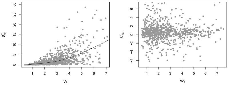
Diagnostic plots for reported daily intakes of folate. The left panel shows the plot of W̄ vs $S_W^2$ with a simple lowess fit superimposed. The right panel shows the plot of W₄ vs C₁₂₃.

5.2 Results for Daily Intakes of Folate

Estimates of the density of daily intakes of folate and other nuisance functions of secondary importance produced by different deconvolution models are summarized in Figure 4. When the density of scaled errors is allowed to be flexible, as in Model-III, the estimated density of daily folate intakes is visibly very different from the estimates when the measurement errors are assumed to be normally or skew-normally distributed, as in Model-I, Model-II or the SRB model, particularly in the interval of 3–6 mcg. Estimated 90% credible intervals for f_X(3.7) for Model-I is (0.167, 0.283), for Model-II is (0.237, 0.375), and for Model-III is (0.092, 0.163). Since the credible interval for Model-III is disjoint from the credible intervals for the other models, the differences in the estimated densities at 3.7 may be considered to be significant.

Figure 4.

Results for data on daily folate intakes from EATS example. The top panel shows the estimated densities of daily folate intake under different models. The bottom left panel shows estimated densities of scaled errors under Model-II (dashed line) and Model-III (solid bold line) superimposed over a standard Normal density (solid line). The bottom right panel shows estimated variance functions under different models. The gray dots represent subject-specific sample means (x-axis) and variances (y-axis). For the top panel and the bottom right panel, the solid thin line is for Model-I; the dashed line is for Model-II; the solid bold line is for Model-III; and the dot-dashed line is for the Model of Staudenmayer, et al. (2008).

Our analysis also showed that the measurement error distributions of all dietary components included in the EATS study deviate from normality and exhibit strong conditional heteroscedasticity. These findings emphasize the importance of flexible conditionally heteroscedastic error distribution models in nutritional epidemiologic studies.

6 Summary and Discussion

6.1 Summary

We have considered the problem of Bayesian density deconvolution in the presence of conditionally heteroscedastic measurement errors. Attending to the specific needs of deconvolution problems, three different approaches were considered for modeling the distribution of measurement errors. The first model made the conventional normality assumption about the measurement errors. The next two models allowed, with varying degrees of flexibility, the distribution of measurement errors to deviate from normality. In all these models conditional heteroscedasticity was also modeled nonparametrically. The proposed methodology, therefore, makes important contributions to the density deconvolution literature, allowing both the distribution of interest and the distribution of measurement errors to deviate from standard parametric laws, while at the same time accommodating conditional heteroscedasticity. Efficiency of the models in recovering the true density of interest was illustrated through simulation experiments, and in particular we showed that our method vastly dominates that of Staudenmayer, et al. (2008). Results of the simulation experiments suggested that all the models introduced in this article out-perform previously existing methods, even while relaxing some of the restrictive assumptions of previous approaches. Simulation experiments also showed that our Bayesian semiparametric deconvolution approaches proposed in this article will often be more efficient than possible nonparametric alternatives, even when the true data generating process deviates from the assumed semiparametric framework.

6.2 Data Transformation and Homoscedasticity

In our application area of nutrition, many researchers assume that W is unbiased for X in the original scale that the nutrient is measured, i.e., E(WjX) = X as in our model, see Willett (1998), Spiegelman, et al. (1997, 2001, 2005) and Kipnis, et al. (2009). It is this original scale of X then that is of scientific interest in this instance. An alternative technique is a transform-retransform method: attempt to transform the W_ij data to make it additive and with homoscedastic measurement error, fit in the transformed scale, and then back-transform the density. For example, if $W_{ij}=X_{i}exp(U_{ij}-{\sigma }_u^2/2)$ where $U_{ij}=\text{Normal}(0,{\sigma }_u^2)$, then $log(W_{ij})=log(X_i)-{\sigma }_u^2/2+U_{ij}$, the classical homoscedastic deconvolution problem with target $X_{\ast }=log(X)-{\sigma }_u^2/2$. One could then use any homoscedastic deconvolution method to estimate the density of X_*, and then from that estimate the density of X. Our methods obviously apply to such a problem. We have used the kernel deconvolution R package “decon” (Wang and Wang, 2011), the only available set of programs, and compared it to our method both using transform-retransform with homoscedasticity and by working in the original scale, using Model III. In a variety of target distributions for X and a variety of sample sizes, our methods consistently have substantially lower MISE.

It is also the case though that transformations to a model such as h(W) = h(X) + U with $U=\text{Normal}(0,{\sigma }_u^2)$ do not satisfy the unbiasedness condition in the original scale. In the log-transformation case, there is a multiplicative bias, but in the cube-root case, $E(W)=E(X)+3{\sigma }_u^{2}E(X^{1/3})$, a model that many in nutrition would find uncomfortable and, indeed, objectionable.

Of course, other fields would be amenable to unbiasedness on a transformed scale, and hope that the measurement error is homoscedastic on that scale. Even in this problem, our methodology is novel and dominates other methods that have been proposed previously. Our methods apply to this problem, allowing flexible Bayesian semiparametric models for the density of X in the transformed scale, flexible Bayesian semiparametric models for the density of the measurement errors, and, if desired, at the same time build modeling robustness lest there be any remaining heteroscedasticity. We have experimented with this ideal case, and even here our methods substantially dominate those currently in the literature. It also must be remembered too that it is often not possible to transform to additivity with homoscedasticity: one example in the EATS data of Section 5, where this occurs with vitamin B for the Box-Cox family. Details are available from the first author.

6.3 Extensions

Application of the Bayesian semiparametric methodology, introduced in this article for modeling conditionally heteroscedastic errors with unknown distribution where the conditioning variable is not precisely measured, is not limited to deconvolution problems. An important extension of this work and the subject of an ongoing research project is an application of the proposed methodology to errors-in-variables regression problems.

Appendix A Model Identifiability

Hu and Schennach (2008) showed that models such as ours are identified under very weak conditions. They show that when four variables, (Y, W, Z, X), where X is the only unobserved variate, are continuously distributed, their joint distribution is identified under the following conditions; their conditions are even weaker, but these suffice for our case.

Conditions 1

1. f_Y|W,Z,X = f_Y|X. 2. f_W|Z,X = f_W|X. 3. (W | X) = X. 4. The set {Y: f_Y|X(Y | X₁) ≠ f_Y|X(Y | X₂)} has positive probability under the marginal of Y for all X₁ ≠ X₂. 5. The marginal, joint and conditional densities of (Y, W, Z, X) are bounded.

They also have a highly technical assumption about injectivity of operators, which is satisfied if the distributions of W given X and Z given X are complete. This means, for example, that if ∫ g(W)f_W|X(W | X)dW = 0 for all X, then g ≡ 0. This is a weak assumption and we comment upon it no further.

When m_i ≥ 3, identifiability of our model (1)–(2) is assured as it falls within the general framework of Hu and Schennach (2008). To see this, replace their Y_i by our W_i1, their W_i by our W_i2, their Z_i by our W_i3 and their X_i by our X_i. Conditions 3.1–3.4 then follow from the fact that (ε_i1, ε_i2, ε_i3, X_i) have a continuous distribution and are mutually independent with E(ε_ij) = 0. Condition 3.5 follows assuming the variance function v is continuous.

We conjecture that model (1)–(2) is identifiable even with m_i ≥ 2 under very weak assumptions. We have numerical evidence to support the claim.

Appendix B Choice of Hyper-Parameters

For the DPMM prior for f_X, the prior variance of each ${\sigma }_k^2$ is ${\sigma }_0^4/\{{({\gamma }_0-2)}^2({\gamma }_0-1)\}$, whereas the prior variance of each μ_k, given ${\sigma }_k^2$ is ${\sigma }_k^2/{\nu }_0$. Small values of γ₀ and ν₀ imply large prior variance and hence non-informativeness. We chose γ₀ = 3 and ν₀ = 1/5. The prior marginal mean and variance of X, obtained by integrating out all but the hyper-parameters, are given by μ₀ and ${\sigma }_0^2(1+1/{\nu }_0)/({\gamma }_0-1)$ respectively. Taking an empirical Bayes type approach, we set μ₀ = W̄ and ${\sigma }_0^2=S_{\mathbf{W}}^2({\gamma }_0-1)/(1+1/{\nu }_0)$, where W̄ is the mean of the subject-specific sample means W̄_1:n, and $S_{\mathbf{W}}^2$ is an estimate of the across subject variance from a one way random effects model. To ensure noninformativeness, hyper-parameters appearing in the prior for f_ε are chosen as σ_μ̃ = 3, a_ε = 1 and b_ε = 1. For real world applications, the values of A and B may not be known. We set [A, B] = [min(W̄_1:n) − 0.1 range(W̄_1:n), max(W̄_1:n) + 0.1 range(W̄_1:n)]. The DP concentration parameters α_X and α_ε could have been assigned gamma hyper-priors (Escobar and West, 1995), but in this article we kept them fixed at α_X = 0.1 and α_ε = 1, respectively. The prior mean and standard deviation of λ were set at μ_0λ= 0 and σ_0λ = 4. For modeling the variance functions v and ṽ, quadratic (q=2) B-splines based are used. See the supplementary materials for detailed expressions. The B-splines are based on (2 × 2 + 10 + 1) = 15 knot points that divide the interval [A, B] into K = 10 subintervals of equal length. We take X₀ = t₅. The identifiability restriction on the variance function for Model III now becomes {exp(ξ₃) + exp(ξ₄)} = 2. The inverse-gamma hyper-prior on the smoothing parameter ${\sigma }_{\xi }^2$ is non-informative if b_ξ is small relative to ξ^TPξ. We chose a_ξ = b_ξ = 0.1.

Appendix C Posterior Inference

Define cluster labels C_1:n, where C_i = k if X_i is associated with the k^th component of the DPMM. Similarly for Model-III, define cluster labels ${\{Z_{ij}\}}_{i,j=1}^{n,m_i}$, where Z_ij = k if ε_ij comes from the k^th component of (14). Let $N={\sum }_{i=1}^n{m}_i$ denote the total number of observations. With a slight abuse of notation, define ${\mathbf{W}}_{1:N}={\{W_{ij}\}}_{i,j=1}^{n,m_i}$ and ${\mathbf{Z}}_{1:N}={\{Z_{ij}\}}_{i,j=1}^{n,m_i}$. Then for Model-I, f_W|X(W_ij | X_i, ξ) = Normal {W_ij | X_i, v(X_i, ξ)}; for Model-II, f_W|X(W_ij | X_i, ξ, λ) = SN{W_ij | X_i, v(X_i, ξ), λ}; and for Model-III, given Z_ij = k, $f_{W\mid X}(W_{ij}\mid X_i,\mathit{\xi },p_k,{\mu }_{k1},{\mu }_{k2},{\sigma }_{k1}^2,{\sigma }_{k2}^2)=p_k\text{Normal}\{W_{ij}\mid X_i+\stackrel{\sim }{v}{(X_i,\mathit{\xi })}^{1/2}{\mu }_{k1},\stackrel{\sim }{v}(X_i,\mathit{\xi }){\sigma }_{k1}^2\}+(1-p_k)\text{Normal}\{W_{ij}\mid X_i+\stackrel{\sim }{v}{(X_i,\mathit{\xi })}^{1/2}{\mu }_{k2},\stackrel{\sim }{v}(X_i,\mathit{\xi }){\sigma }_{k2}^2\}$. In what follows ζ denotes a generic variable that collects all other parameters of a model, including X_1:n, that are not explicitly mentioned.

It is possible to integrate out the random mixture probabilities from the prior and posterior full conditionals of the cluster labels. Classical algorithms for fitting DPMMs make use of this and work with the resulting Polya urn scheme. Neal (2000) provided an excellent review of this type of algorithm for both conjugate and non-conjugate cases. In this article, the parameters specific to DPMMs are updated using algorithms specific to those models and other parameters are updated using the Metropolis-Hastings algorithm. In what follows, the generic notation q(current → proposed) denotes the proposal distributions of the Metropolis-Hastings steps proposing a move from the current value to the proposed value.

The starting values of the MCMC chain are determined as follows. Subject-specific sample means W̄_1:n are used as starting values for X_1:n. Each C_i is initialized at i with each X_i coming from its own cluster with mean μ_i = X_i and variance ${\sigma }_i^2={\sigma }_0^2$. In addition, ${\sigma }_{\xi }^2$ is initialized at 0.1. The initial value of ξ is obtained by maximizing ℓ(ξ | 0.1, W̄_1:n) with respect to ξ, where $\ell (\mathit{\xi }\mid {\sigma }_{\xi }^2,{\mathbf{X}}_{1:n})$ denotes the conditional log-posterior of ξ. The parameters of the distribution of scaled errors are initialized at values that correspond to the special standard normal case. For example, for Model-II, λ is initialized at zero. For Model-III, Z_ij’s are all initialized at 1 with $(p_1,{\stackrel{\sim }{\mu }}_1,{\sigma }_{11}^2,{\sigma }_{12}^2)=(0.5,0,1,1)$. The MCMC iterations comprise the following steps.

1. Updating the parameters of the distribution of X: Conditionally given X_1:n, the parameters specifying the DPMM for f_X can be updated using a Gibbs sampler (Neal, 2000, Algorithm 2). The full conditional of C_i is given by

   $$\begin{array}{c}p(C_i=k,k\in {\mathbf{C}}_{-i}\mid {\mathbf{X}}_{1:n},{\mathbf{C}}_{-i},\mathit{\zeta })=b\frac{n_{-i,k}}{n-1+{\alpha }_X}\text{Normal}(X_i\mid {\mu }_k,{\sigma }_k^2),\\ p(C_i\notin {\mathbf{C}}_{-i}\mid {\mathbf{X}}_{1:n},{\mathbf{C}}_{-i},\mathit{\zeta })=b\frac{{\alpha }_X}{n-1+{\alpha }_X}{\mathrm{t}}_{2{\gamma }_0}(t_i),\end{array}$$

   where b denotes the appropriate normalizing constant; for each i, C_−i = C_1:n −{C_i}; n_−i,k =Σ_{l:l≠i}1_{cl=k} is the number of c_l’s that equal k in C_−i; and $t_i={\gamma }_0^{1/2}(X_i-{\mu }_0)/\{{\sigma }_0{(1+1/{\nu }_0)}^{1/2}\}$. t_m denotes the density of a t-distribution with m degrees of freedom.

   For all k ∈ C_1:n, we update (μ_k, ${\sigma }_k^2$) using the closed-form joint full conditional given by $\{({\mu }_k,{\sigma }_k^2\mid {\mathbf{X}}_{1:n},\mathit{\zeta })\}=\text{NIG}({\mu }_{nk},{\sigma }_{nk}^2/{\nu }_{nk},{\gamma }_{nk},{\sigma }_{nk}^2)$, where $n_k={\sum }_{i=1}^n{1}_{\{C_i=k\}}$is the number of X_i’s associated with the k^th cluster; ν_nk = (ν₀ + n_k); γ_nk = (γ₀ + n_k/2); μ_nk = (ν₀μ₀ + n_kΣ_{i:Ci=k} X_i)/(ν₀ + n_k) and ${\sigma }_{nk}^2={\sigma }_0^2+({\sum }_{\{i:C_i=k\}}{X}_i^2+{\nu }_0{\mu }_0^2-{\nu }_{nk}{\mu }_{nk}^2)/2$.

2. Updating X_1:n: Because the X_i’s are conditionally independent, the full conditional of X_i is given by $p(X_i\mid {\mathbf{W}}_{1:N},\mathit{\zeta })\propto {\widehat{f}}_X(X_i\mid \mathit{\zeta })\times {\prod }_{j=1}^{m_i}{f}_{W\mid X}(W_{ij}\mid X_i,\mathit{\zeta })$. We use a Metropolis-Hastings sampler to update the X_i’s with proposal $q(X_i\to X_{i,\mathit{new}})=TN(X_{i,\mathit{new}}\mid X_i,{\sigma }_X^2,[A,B])$, where σ_X = (the range of W̄_1:n)/6 and TN(· | m, s², [ℓ,u]) denotes a truncated normal distribution with location m and scale s restricted to the interval [ℓ, u].

3. Updating the parameters of the distribution of scaled errors: For Model-II and Model-III, the parameters involved in the distribution of scaled errors have to be updated.

   For Model-II, the distribution of scaled error is SN(0, 1, λ), involving only the parameter λ. The full conditional of λ is given by $p(\lambda \mid {\mathbf{W}}_{1:N},\mathit{\zeta })\propto p_0(\lambda )\times {\prod }_{i=1}^n{\prod }_{j=1}^{m_i}{f}_{W\mid X}(W_{ij}\mid \lambda ,\mathit{\zeta })$. We use Metropolis-Hastings sampler to update λ with random walk proposal $q(\lambda \to {\lambda }_{\mathit{new}})=\text{Normal}({\lambda }_{\mathit{new}}\mid \lambda ,{\sigma }_{\lambda }^2)$.

   For Model-III, we use Metropolis-Hastings samplers to update the latent parameters Z_1:N as well as the component specific parameters (p_k, μ̃_k, ${\sigma }_{k1}^2,{\sigma }_{k2}^2$)’s (Neal, 2000, Algorithm 5). We propose a new value of Z_ij, say Z_ij,_new, according to its marginalized conditional prior

   $$\begin{array}{c}p(Z_{ij}=k,k\in {\mathbf{Z}}_{-ij}\mid {\mathbf{Z}}_{-ij})=N_{-ij,k}/(N-1+{\alpha }_{\epsilon }),\\ p(Z_{ij}\notin {\mathbf{Z}}_{-ij}\mid {\mathbf{Z}}_{-ij})={\alpha }_{\epsilon }/(N-1+{\alpha }_{\epsilon }),\end{array}$$
   where, for each (i, j) pair, Z_−ij = Z_1:N − {Z_ij}; N_−ij,k = Σ_[rs:rs≠ij} 1_{Zrs=k}, the number of Z_rs’s in Z_−ij that equal k. If Z_ij,_new ∉ Z_−ij, we draw (pZ_ij,_new, μ̃Z_ij,_new, ${\sigma }_{Z_{ij,\mathit{new}}1}^2,{\sigma }_{Z_{ij,\mathit{new}}2}^2$) from the prior p₀(p, μ̃, ${\sigma }_1^2,{\sigma }_2^2$. We update Z_ij to its proposed value with probability

   $$min\left\{1,\frac{f_{W\mid X}(W_{ij}\mid p_{Z_{ij,\mathit{new}}},{\stackrel{\sim }{\mu }}_{Z_{ij,\mathit{new}}},{\sigma }_{Z_{ij,\mathit{new}}1}^2,{\sigma }_{Z_{ij,\mathit{new}}2}^2,\mathit{\zeta })}{f_{W\mid X}(W_{ij}\mid p_{Z_{ij}},{\stackrel{\sim }{\mu }}_{Z_{ij}},{\sigma }_{Z_{ij}1}^2,{\sigma }_{Z_{ij}2}^2,\mathit{\zeta })}\right\}.$$
   For all k ∈ Z_1:N, we propose a new value for (p_k, μ̃_k, ${\sigma }_{k1}^2,{\sigma }_{k2}^2$) with the proposal $q\{{\mathit{\theta }}_k=(p_k,{\stackrel{\sim }{\mu }}_k,{\sigma }_{k1}^2,{\sigma }_{k2}^2)\to (p_{k,\mathit{new}},{\stackrel{\sim }{\mu }}_{k,\mathit{new}},{\sigma }_{k1,\mathit{new}}^2,{\sigma }_{k2,\mathit{new}}^2)={\mathit{\theta }}_{k,\mathit{new}}\}=\text{TN}(p_{k,\mathit{new}}\mid p_k,{\sigma }_p^2,[0,1])\times \text{Normal}({\stackrel{\sim }{\mu }}_{k,\mathit{new}}\mid {\stackrel{\sim }{\mu }}_k,{\sigma }_{\stackrel{\sim }{\mu }}^2)\times \text{TN}({\sigma }_{k1,\mathit{new}}^2\mid {\sigma }_{k1}^2,{\sigma }_{\sigma }^2,[max\{0,{\sigma }_{k1}^2-1\},{\sigma }_{k1}^2+1])\times \text{TN}({\sigma }_{k2,\mathit{new}}^2\mid {\sigma }_{k2}^2,{\sigma }_{\sigma }^2,[max\{0,{\sigma }_{k2}^2-1\},{\sigma }_{k2}^2+1])$. We update θ_k to the proposed value θ_k,new with probability

   $$min\left\{1,\frac{q({\mathit{\theta }}_{k,\mathit{new}}\to {\mathit{\theta }}_k)}{q({\mathit{\theta }}_k\to {\mathit{\theta }}_{k,\mathit{new}})}\frac{{\prod }_{\{ij:z_{ij}=k\}}{f}_{W\mid X}(W_{ij}\mid {\mathit{\theta }}_{k,\mathit{new}},\mathit{\zeta })p_0({\mathit{\theta }}_{k,\mathit{new}})}{{\prod }_{\{ij:z_{ij}=k\}}{f}_{W\mid X}(W_{ij}\mid {\mathit{\theta }}_k,\mathit{\zeta })p_0({\mathit{\theta }}_k)}\right\}.$$

4. Updating the parameters of the variance function: The full conditional for ξ is given by $p(\mathit{\xi }\mid {\mathbf{W}}_{1:N},\mathit{\zeta })\propto p_0(\mathit{\xi })\times {\prod }_{i=1}^n{\prod }_{j=1}^{m_i}{f}_{W\mid X}(W_{ij}\mid \mathit{\xi },\mathit{\zeta })$. We use Metropolis-Hastings sampler to update ξ with random walk proposal q(ξ → ξ_new) = MVN(ξ_new | ξ, Σ_ξ). For Model III, the identifiability restriction is imposed by replacing ξ_new,₃ = log{2 − exp(ξ_new,4)}.

   Finally, we update the hyper-parameter ${\sigma }_{\xi }^2$ using its closed-form full conditional $({\sigma }_{\xi }^2\mid \mathit{\xi },\mathit{\zeta })=\text{IG}\{a_{\xi }+(J+2)/2,b_{\xi }+{\mathit{\xi }}^{\prime }P\mathit{\xi }/2\}$.

The covariance matrix Σ_ξ of the proposal distribution for ξ is taken to be the inverse of the negative Hessian matrix of l(ξ | 0.1, W̄_1:n) evaluated at the chosen initial value of ξ. See Appendix D for more details. Other variance parameters appearing in the proposal distributions are tuned to get good acceptance rates for the Metropolis-Hastings samplers, the values σ_λ = 1, σ_p = 0.01 and σ_σ = 0.1 working well in the examples considered. In simulation experiments, 5,000 MCMC iterations with the initial 3,000 discarded as burn-in produced very stable estimates of the density and the variance function.

The posterior estimate of f_X is given by the unconditional predictive density f_X(· | W_1:N). A Monte Carlo estimate of f_X(· | W_1:N), based on M samples from the posterior, is given by

$${\widehat{f}}_X(X\mid {\mathbf{W}}_{1:N})=M^{-1}{\sum }_{m=1}^M[{\sum }_{k=1}^{k^{(m)}}\{n_k^{(m)}/({\alpha }_X+n)\}\text{Normal}(X\mid {\mu }_k^{(m)},{\sigma }_k^{(m)2})+\{{\alpha }_X/({\alpha }_X+n)\}{\mathrm{t}}_{2{\gamma }_0}(t_X)],$$

where $t_X=t(X)={\gamma }_0^{1/2}(X-{\mu }_0)/\{{\sigma }_0{(1+1/{\nu }_0)}^{1/2}\},({\mu }_k^{(m)},{\sigma }_k^{(m)2})$ is the sampled value of (μ_k, ${\sigma }_k^2$) in the m^th sample, $n_k^{(m)}$ is the number of X_i’s associated with the k^th cluster, and k^(m) is the total number of active clusters. With $(p_k^{(m)},{\stackrel{\sim }{\mu }}_k^{(m)},{\sigma }_{k1}^{(m)2},{\sigma }_{k2}^{(m)2}),N_k^{(m)}$ and $k_{\epsilon }^{(m)}$ defined in a similar fashion, the posterior Monte Carlo estimate of f_ε for Model-III is

$$\widehat{f_{\epsilon }}(\epsilon \mid {\mathbf{W}}_{1:N})=M^{-1}{\sum }_{m=1}^M[{\sum }_{k=1}^{k_{\epsilon }^{(m)}}\{N_k^{(m)}/({\alpha }_{\epsilon }+N)\}{f}_{c\epsilon }(\epsilon \mid p_k^{(m)},{\stackrel{\sim }{\mu }}_k^{(m)},{\sigma }_{k1}^{(m)2},{\sigma }_{k2}^{(m)2})+\{{\alpha }_{\epsilon }/({\alpha }_{\epsilon }+N)\}\int f_{c\epsilon }(\epsilon \mid p,\stackrel{\sim }{\mu },{\sigma }_{k1}^2,{\sigma }_{k2}^2){dp}_0(p,\stackrel{\sim }{\mu },{\sigma }_{k1}^2,{\sigma }_{k2}^2)],$$

The integral above can not be exactly evaluated. Monte Carlo approximation may be used. If N ≫ α_ε, the term may simply be neglected. For Model II, f_ε can be estimated by ${\widehat{f}}_{\epsilon }(\epsilon \mid {\mathbf{W}}_{1:N})={\sum }_{m=1}^M\text{SN}(\epsilon \mid 0,1,{\lambda }^{(m)})/M$. For Models I and II, an estimate of the variance function v can similarly be obtained as $\widehat{v}(X\mid {\mathbf{W}}_{1:N})={\sum }_{m=1}^{M}v(X\mid {\mathit{\xi }}^{(m)})/M$. An estimate of the restricted variance function ṽ for Model III can be obtained using a similar formula. For Model III, v̂ and a scaled version of $\widehat{f_{\epsilon }}$, scaled to have unit variance, can be obtained using the estimate of ṽ(X₀).

Appendix D Initial Values and Proposals for ξ

The conditional posterior log-likelihood of ξ for Model-I is given by

$$\ell (\mathit{\xi }\mid {\sigma }_{\xi }^2,{\mathbf{X}}_{1:n})=-\frac{1}{2{\sigma }_{\xi }^2}{\mathit{\xi }}^{\mathrm{T}}P\mathit{\xi }-\sum _{i=1}^n\left\{\frac{m_i}{2}logv(X_i,\mathit{\xi })+\sum _{j=1}^{m_i}\frac{1}{2v(X_i,\mathit{\xi })}{(W_{ij}-X_i)}^2\right\}.$$

The initial values for the M-H sampler for ξ is obtained as ξ ⁽⁰⁾ = arg max ℓ(ξ | 0.1, W̄_1:n). Numerical optimization is performed using the optim routine in R with the analytical gradient supplied.

The covariance matrix of the random walk proposal for ξ is taken to be the inverse of the negative of the matrix of second partial derivatives of ℓ(ξ | 0.1, W̄_1:n) evaluated at ξ ⁽⁰⁾. Expressions for the gradient and the second derivatives are given below.

$$\begin{array}{l}\frac{\partial \ell (\mathit{\xi }\mid {\sigma }_{\xi }^2,{\mathbf{X}}_{1:n})}{\partial {\xi }_k}=-\frac{{(P\mathit{\xi })}_k}{{\sigma }_{\xi }^2}-\sum _{i=1}^n\left\{m_i-\sum _{j=1}^{m_i}\frac{{(W_{ij}-X_i)}^2}{v(X_i,\mathit{\xi })}\right\}\frac{b_{2,k}(X_i)exp({\xi }_k)}{2v(X_i,\mathit{\xi })},\\ \frac{{\partial }^2\ell (\mathit{\xi }\mid {\sigma }_{\xi }^2,{\mathbf{X}}_{1:n})}{\partial {\xi }_k^2}=-\frac{{(P)}_{kk}}{{\sigma }_{\xi }^2}-\sum _{i=1}^n\left\{\sum _{j=1}^{m_i}\frac{{(W_{ij}-X_i)}^2}{v(X_i,\mathit{\xi })}-\frac{m_i}{2}\right\}\frac{b_{2,k}{(X_i)}^2}{v{(X_i,\mathit{\xi })}^2}exp(2{\xi }_k)-\sum _{i=1}^n\left\{m_i-\sum _{j=1}^{m_i}\frac{{(W_{ij}-X_i)}^2}{v(X_i,\mathit{\xi })}\right\}\frac{b_{2,k}(X_i)exp({\xi }_k)}{2v(X_i,\mathit{\xi })},\\ \frac{{\partial }^2\ell (\mathit{\xi }\mid {\sigma }_{\xi }^2,{\mathbf{X}}_{1:n})}{\partial {\xi }_k\partial {\xi }_{k^{\prime }}}=-\frac{{(P)}_{k{k}^{\prime }}}{{\sigma }_{\xi }^2}-\sum _{i=1}^n\left\{\sum _{j=1}^{m_i}\frac{{(W_{ij}-X_i)}^2}{v(X_i,\mathit{\xi })}-\frac{m_i}{2}\right\}\frac{b_{2,k}(X_i)b_{2,k^{\prime }}(X_i)}{v{(X_i,\mathit{\xi })}^2}exp({\xi }_k+{\xi }_{k^{\prime }}).\end{array}$$

References

- Azzalini A. A class of distributions which includes the Normal ones. Scandinavian Journal of Statistics. 1985;12:171–178. [Google Scholar]
- Carroll RJ, Hall P. Optimal rates of convergence for deconvolving a density. Journal of the American Statistical Association. 1988;83:1184–1186. [Google Scholar]
- Carroll RJ, Hall P. Low order approximations in deconvolution and regression with errors in variables. Journal of the Royal Statistical Society, Series B. 2004;66:31–46. [Google Scholar]
- Carroll RJ, Roeder K, Wasserman L. Flexible parametric measurement error models. Biometrics. 1999;55:44–54. doi: 10.1111/j.0006-341x.1999.00044.x. [DOI] [PubMed] [Google Scholar]
- Chan D, Kohn R, Nott D, Kirby C. Locally adaptive semiparametric estimation of the mean and variance functions in regression models. Journal of Computational and Graphical Statistics. 2006;15:915–936. [Google Scholar]
- Chung Y, Dunson DB. Nonparametric Bayes conditional distribution modeling with variable selection. Journal of the American Statistical Association. 2009;104:1646–1660. doi: 10.1198/jasa.2009.tm08302. [DOI] [PMC free article] [PubMed] [Google Scholar]
- de Boor C. A Practical Guide to Splines. New York: Springer; 2000. [Google Scholar]
- Devroye L. Consistent deconvolution in density estimation. Canadian Journal of Statistics. 1989;17:235–239. [Google Scholar]
- Eckert RS, Carroll RJ, Wang N. Transformations to additivity in measurement error models. Biometrics. 1997;53:262–272. [PubMed] [Google Scholar]
- Eilers PHC, Marx BD. Flexible smoothing with B-splines and penalties. Statistical Science. 1996;11:89–121. [Google Scholar]
- Escobar MD, West M. Bayesian density estimation and inference using mixtures. Journal of the American Statistical Association. 1995;90:577–588. [Google Scholar]
- Fan J. On the optimal rates of convergence for nonparametric deconvolution problems. Annals of Statistics. 1991a;19:1257–1272. [Google Scholar]
- Fan J. Global behavior of deconvolution kernel estimators. Statistica Sinica. 1991b;1:541–551. [Google Scholar]
- Fan J. Deconvolution with supersmooth distributions. Canadian Journal of Statistics. 1992;20:155–169. [Google Scholar]
- Ferguson TF. A Bayesian analysis of some nonparametric problems. Annals of Statistics. 1973;1:209–230. [Google Scholar]
- Hesse CH. Data driven deconvolution. Journal of Nonparametric Statistics. 1998;10:343–373. [Google Scholar]
- Hu Y, Schennach SM. Instrumental variable treatment of nonclassical measurement error models. Econometrica. 2008;76:195–216. [Google Scholar]
- Kipnis V, Midthune D, Buckman DW, Dodd KW, Guenther PM, Krebs-Smith SM, Subar AF, Tooze JA, Carroll RJ, Freedman LS. Modeling data with excess zeros and measurement error: application to evaluating relationships between episodically consumed foods and health outcomes. Biometrics. 2009;65:1003–1010. doi: 10.1111/j.1541-0420.2009.01223.x. [DOI] [PMC free article] [PubMed] [Google Scholar]
- Li T, Vuong Q. Nonparametric estimation of the measurement error model using multiple indicators. Journal of Multivariate Analysis. 1998;65:139–165. [Google Scholar]
- Liu A, Tong T, Wang Y. Smoothing spline estimation of variance functions. Journal of Computational and Graphical Statistics. 2006;16:312–329. [Google Scholar]
- Liu MC, Taylor RL. A consistent nonparametric density estimator for the decon-volution problem. Canadian Journal of Statistics. 1989;17:427–438. [Google Scholar]
- Lo AY. On a class of Bayesian nonparametric estimates. I: Density estimates. Annals of Statistics. 1984;12:351–357. [Google Scholar]
- Neal RM. Markov chain sampling methods for Dirichlet process mixture models. Journal of Computational and Graphical Statistics. 2000;9:249–265. [Google Scholar]
- Pelenis J. Semiparametric Bayesian regression. Journal of Econometrics. 2014;178:624–638. [Google Scholar]
- Sethuraman J. A constructive definition of Dirichlet priors. Statistica Sinica. 1994;4:639–650. [Google Scholar]
- Spiegelman D, McDermott A, Rosner B. The regression calibration method for correcting measurement error bias in nutritional epidemiology. American Journal of Clinical Nutrition. 1997;65 (supplement):1179S–1186S. doi: 10.1093/ajcn/65.4.1179S. [DOI] [PubMed] [Google Scholar]
- Spiegelman D, Carroll RJ, Kipnis V. Efficient regression calibration for logistic regression in main study/internal validation study designs with an imperfect reference instrument. Statistics in Medicine. 2001;20:139–160. doi: 10.1002/1097-0258(20010115)20:1<139::aid-sim644>3.0.co;2-k. [DOI] [PubMed] [Google Scholar]
- Spiegelman D, Zhao B, Kim J. Correlated errors in biased surrogates: study designs and methods for measurement error correction. Statistics in Medicine. 2005;24:1657–1682. doi: 10.1002/sim.2055. [DOI] [PubMed] [Google Scholar]
- Staudenmayer J, Ruppert D, Buonaccorsi JP. Density estimation in the presence of heteroscedastic measurement error. Journal of the American Statistical Association. 2008;103:726–736. [Google Scholar]
- Suber AF, Thompson FE, Kipnis V, Midthune D, Hurwitz P, McNutt S, McIntosh A, Rosenfeld S. Comparative validation of the block, Willet, and National Cancer Institute food frequency questionnaires. American Journal of Epidemiology. 1990;154:1089–1099. doi: 10.1093/aje/154.12.1089. [DOI] [PubMed] [Google Scholar]
- Wang X, Wang B. Deconvolution estimation in measurement error models: the R package decon. Journal of Statistical Software. 2011;39:1–24. [PMC free article] [PubMed] [Google Scholar]
- West M, Müller P, Escobar MD. Hierarchical priors and mixture models, with application in regression and density estimation. In: Smith AFM, Freeman P, editors. Aspects of uncertainty: a tribute to D. V. Lindley. New York: Wiley; 1994. pp. 363–386. [Google Scholar]
- Willett W. Nutritional Epidemiology. 2. Oxford University Press; 1998. [Google Scholar]
- Yau P, Kohn R. Estimation and variable selection in nonparametric heteroscedastic regression. Statistics and Computing. 2003;13:191–208. [Google Scholar]
- Zaykin DV, Zhivotovsky LA, Westfall PH, Weir BS. Truncated product method for combining p-values. Genetic Epidemiology. 2002;22:170–185. doi: 10.1002/gepi.0042. [DOI] [PubMed] [Google Scholar]
Associated Data
This section collects any data citations, data availability statements, or supplementary materials included in this article.