A unification of mediation and interaction: a four-way decomposition

Abstract

It is shown that the overall effect of an exposure on an outcome, in the presence of a mediator with which the exposure may interact, can be decomposed into four components: (i) the effect of the exposure in the absence of the mediator, (ii) the interactive effect when the mediator is left to what it would be in the absence of exposure, (iii) a mediated interaction, and (iv) a pure mediated effect. These four components, respectively, correspond to the portion of the effect that is due to neither mediation nor interaction, to just interaction (but not mediation), to both mediation and interaction, and to just mediation (but not interaction). This four-way decomposition unites methods that attribute effects to interactions and methods that assess mediation. Certain combinations of these four components correspond to measures for mediation, while other combinations correspond to measures of interaction previously proposed in the literature. Prior decompositions in the literature are in essence special cases of this four-way decomposition. The four-way decomposition can be carried out using standard statistical models, and software is provided to estimate each of the four components. The four-way decomposition provides maximum insight into how much of an effect is mediated, how much is due to interaction, how much is due to both mediation and interaction together, and how much is due to neither.

Methodology for assessing mediation and interaction has developed rapidly over the past decade. Methods for effect decomposition to assess direct and indirect effects have shed light on mechanisms and pathways.^1–19 Other methods and measures have been useful in assessing how much of the effect of one exposure is due to its interaction with another.^20–24 This paper provides theory and methods to unite these effect-decomposition and effect-attribution methods for mediation and interaction. The paper’s central result is that the total effect of an exposure on an outcome, in the presence of a mediator with which the exposure may interact, can be decomposed into components due to just mediation, to just interaction, to both mediation and interaction, and to neither mediation nor interaction.

After presenting this four-way decomposition, this paper discusses assumptions for identifying these four components from data and relates this four-way decomposition approach to various statistical models. The paper discusses the relations between existing measures of mediation and interaction and each of the four components, and shows how existing measures of mediation and interaction consist of different combinations of these four components. Different effect decomposition and attribution approaches for mediation and interaction can in fact be united within this four-fold framework. When some of the components are combined, the framework presented here essentially collapses into approaches used previously. The greatest insight, however, is arguably gained when the four-fold approach is employed as illustrated with an example from genetic epidemiology.

Notation

Let A denote the exposure of interest, Y the outcome, and M a potential mediator, and let C denote a set of baseline covariates. Suppose we want to compare two levels of the exposure, a and a^*; for binary exposure we would have a = 1 and a^* = 0. For simplicity, consider the setting of a binary exposure and binary mediator; more general results that are applicable to arbitrary exposures and mediators are given in the Appendix. Let Y_a and M_a denote respectively the potentially counterfactual values of the outcome and mediator that would have been observed had the exposure A been set to level a. The total effect (TE) of the exposure A on the outcome Y is defined as Y₁ − Y₀; the total effect of the exposure A on the mediator M is defined as M₁ − M₀. We will not, in general, ever know what these effects are at the individual level but we might hope to be able to estimate them on average for a population. For the first part of this paper, however, will be concerned with concepts, and will later address what can be identified with data and under what assumptions.

Counterfactuals of another form will also be needed. Let Y_am denote the value of the outcome that would have been observed had A been set to level a, and M to m. The controlled direct effect, comparing exposure level A = 1 to A = 0 and fixing the mediator to level m, is defined by Y_1m − Y_0m and captures the effect of exposure A on outcome Y, intervening to fix M to m; it may be different for different levels of m.^1,2 It may also be different for persons. Finally we will also later consider counterfactuals of the form Y_aMa³ which is the outcome Y that would have occurred if A were fixed to a, and if M were fixed to the level it would have taken if A had been a^*. Some technical assumptions referred to as consistency and composition are also needed to relate the observed data to counterfactual quantities. The consistency assumption in this context is that when A = a, the counterfactual outcomes Y_a and M_a are equal to the observed outcomes Y and M, respectively, and that when A = a and M = m, the counterfactual outcome Y_am is equal to Y. The composition assumption is that Y_a = Y_aMa. Further discussion of these assumptions is given elsewhere.^4,18,25

A Four-Fold Decomposition

In the Appendix it is shown that a total effect (TE) of A on Y can be decomposed into the following four components:

$$Y_1-Y_0=(Y_{10}-Y_{00})+(Y_{11}-Y_{10}-Y_{01}+Y_{00})(M_0)+(Y_{11}-Y_{10}-Y_{01}+Y_{00})(M_1-M_0)+(Y_{01}-Y_{00})(M_1-M_0).$$ (1)

The first component, (Y₁₀ −Y₀₀), is the direct effect of the exposure A if the mediator were removed, i.e. fixed to M = 0. This effect is sometimes referred to as a “controlled direct effect” (CDE).^1,2 The second component, (Y₁₁ − Y₁₀ − Y₀₁ + Y₀₀)(M₀), will be referred to as a “reference interaction” (INT_ref). The term (Y₁₁ − Y₁₀ − Y₀₁ + Y₀₀) is an additive interaction. It can be rewritten as (Y₁₁ − Y₀₀) − {(Y₁₀ − Y₀₀) + (Y₀₁ − Y₀₀)} and will be non-zero for a person if the effect on the outcome of setting both the exposure and the mediator to present differs from the sum of the effect of having only the exposure present and the effect of having only the mediator present; additive interaction is generally considered of greatest public health importance.^20–22 The second component in the decomposition in (1) is the product of this additive interaction and M₀. Thus this second component, (Y₁₁ − Y₁₀ − Y₀₁ + Y₀₀)(M₀), is an additive interaction that operates only if the mediator is present in the absence of exposure i.e. when M₀ = 1. The third component, (Y₁₁ − Y₁₀ − Y₀₁ + Y₀₀)(M₁ − M₀), will be referred to as a “mediated interaction” (INT_med). It is the same additive interaction contrast multiplied by (M₁ − M₀). In other words, it is an additive interaction that operates only if the exposure has an effect on the mediator so that M₁ − M₀ ≠ 0. The final component, (Y₀₁ − Y₀₀)(M₁ − M₀), is the effect of the mediator in the absence of the exposure, Y₀₁ − Y₀₀, multiplied by the the effect of the exposure on the mediator itself, M₁ − M₀. It will be non-zero only if the mediator affects the outcome when the exposure is absent, and the exposure itself affects the mediator. This final component could be referred to as a “mediated main effect” or (as explained below) a “pure indirect effect” (PIE).^1,2

The intuition behind this decomposition is that if the exposure affects the outcome for a particular individual, then at least one of four things must be the case. One, the exposure might affect the outcome through pathways that do not require the mediator (i.e. the exposure affects the outcome even when the mediator is absent); in other words the first component is non-zero. Two, the exposure effect might operate only in the presence of the mediator (i.e. there is an interaction), with the exposure itself not necessary for the mediator to be present (i.e. the mediator itself would be present in the absence of the exposure, though the mediator is itself necessary for the exposure to have an effect on the outcome); in other words, the second component is non-zero. A third possibility is that the exposure effect might operate only in the presence of the mediator (i.e. there is an interaction), with the exposure itself needed for the mediator to be present (i.e. the exposure causes the mediator, and the presence of the mediator is itself necessary for the exposure to have an effect on the outcome); in other words, the third component in non-zero. The fourth possibility is that the mediator can cause the outcome in the absence of the exposure, but the exposure is necessary for the mediator itself to be present; in other words, the fourth component is non-zero. The decomposition above, proved in the Appendix, provides a mathematical formalization of this intuition. We could thus rewrite our decomposition as:

$$TE=\mathit{CDE}+{\mathit{INT}}_{\mathit{ref}}+{\mathit{INT}}_{\mathit{med}}+\mathit{PIE}.$$

As with the total effect of the exposure on the outcome, Y₁ − Y₀, it is not in general possible to know the value of each of the four components for a particular individual, but (as discsussed below) there are assumptions under which measures of these four components on average can be estimated for a particular population. As shown below, there are certain assumptions about confounding under which the average value of each of four components is given by the following empirical expressions:

$$\begin{array}{l}E[\mathit{CDE}]=(p_{10}-p_{00})\\ E[{\mathit{INT}}_{\mathit{ref}}]=(p_{11}-p_{10}-p_{01}+p_{00})P(M=1\mid A=0)\\ E[{\mathit{INT}}_{\mathit{med}}]=(p_{11}-p_{10}-p_{01}+p_{00})\{P(M=1\mid A=1)-P(M=1\mid A=0)\}\\ E[\mathit{PIE}]=(p_{01}-p_{00})\{P(M=1\mid A=1)-P(M=1\mid A=0)\}.\end{array}$$

where p_am = E(Y|A = a, M = m). Letting p_a = E(Y|A = a) produces the following empirical decomposition:

$$\begin{array}{l}{p}_{a=1}-p_{a=0}=(p_{10}-p_{00})+(p_{11}-p_{10}-p_{01}+p_{00})P(M=1\mid A=0)\\ +(p_{11}-p_{10}-p_{01}+p_{00})\{P(M=1\mid A=1)-P(M=1\mid A=0)\}\\ +(p_{01}-p_{00})\{P(M=1\mid A=1)-P(M=1\mid A=0)\}\end{array}$$ (1b)

With such average measures it is possible to assess how much of the total effect is due to neither mediation nor interaction (the first component); how much is due to interaction but not mediation (the second component); how much is due to both mediation and interaction (the third component); and how much of the effect is due to mediation but not interaction (the fourth component). The four components of the total effect are summarized in Table 1. Letting E[TE] denote the average total effect for the population (equal to p_a=1 − p_a=0 = E(Y|A = 1) − E(Y|A = 0) in the absence of confounding), then the proportion of the total effect that is due to each of these four components can be expressed using the ratios $\frac{E[\mathit{CDE}]}{E[TE]},\frac{E[{\mathit{INT}}_{\mathit{ref}}]}{E[TE]},\frac{E[{\mathit{INT}}_{\mathit{med}}]}{E[TE]}$, and $\frac{E[\mathit{PIE}]}{E[TE]}$. We could also assess the overall proportion due to mediation by summing the proportions due to the mediated interaction and to the pure indirect effect, i.e. $\frac{E[{\mathit{INT}}_{\mathit{med}}]+E[\mathit{PIE}]}{E[TE]}$. Similarly, the overall proportion due to interaction can be assessed by summing the proportions due to the reference interaction and to the mediated interaction, i.e. $\frac{E[{\mathit{INT}}_{\mathit{ref}}]+E[{\mathit{INT}}_{\mathit{med}}]}{E[TE]}$. Reporting such proportion measures, however, generally makes sense only if all of the components are in the same direction (e.g. all positive or all negative). The statistical properties of such proportion measures can also be highly variable (and hence problematic) if the total effect is close to zero, as might be the case if some of the components were positive and others negative. Similar comments pertain to other proportion measures described below.

Table 1.

The Four Basic Components of the Total Effect (the following four components sum to the total effect TE = Y₁ − Y₀)

Effect	Counterfactual Definition	Empirical Analogue	Interpretation
Controlled Direct Effect (CDE)	(Y10 − Y00)	(p10 − p00)	Due Neither to Mediation nor Interaction
Reference Interaction (INTref)	(Y11 − Y10 − Y01 + Y00)(M0)	(p11 − p10 − p01 + p00)P(M = 1|A = 0)	Due to Interaction Only
Mediated Interaction (INTmed)	(Y11 − Y10 − Y01 + Y00)(M1 − M0)	(p11 − p10 − p01 + p00){P(M = 1|A = 1) − P(M = 1|A = 0)}	Due to Mediation and Interaction
Pure Indirect Effect (PIE)	(Y01 − Y00)(M1 − M0) = (Y0M1 − Y0M0)	(p01 − p00){P(M = 1|A = 1) − P(M = 1|A = 0)}.	Due to Mediation Only

The following section considers the no-confounding assumptions that allow estimation of these four components on average, and the sections after that the statistical methods to carry out such estimation. Later sections consider the relationships between this four-fold decomposition and other concepts from the literatures on mediation and interaction that involve effect decomposition and attribution.

Identification of the Effects

The discussion thus far has been primarily conceptual. As noted, the individual-level effects in the four-way decomposition cannot be identified from the data, but under certain no-confounding assumptions the four components can be identified from the data on average for a population. As discussed further in the Appendix, for a causal diagram interpreted as non-parametric structural equation models of Pearl,¹⁸ the following four assumptions suffice to identify each of the four components from the data: (i) the effect the exposure A on the outcome Y is unconfounded conditional on C; (ii) the effect the mediator M on the outcome Y is unconfounded conditional on (C, A); (iii) the effect the exposure A on the mediator M is unconfounded conditional on C; and (iv) none of the mediator-outcome confounders are themselves affected by the exposure. These are the same four assumptions often used in the literature on mediation.^2,4,5 Letting X ⫫ Y|Z denote that X is independent of Y conditional on Z, then these four assumptions stated formally in terms of counterfactual independence are: (i) Y_am ⫫ A|C, (ii) Y_am ⫫ M|{A, C}, (iii) M_a ⫫ A|C, and (iv) Y_am ⫫ M_a^*|C. Note that assumption (iv) requires that none of the mediator-outcome confounders are themselves affected by the exposure. This assumption would hold in Figure 1 but would be violated in Figure 2. If these four assumptions held without covariates, then we would have the empirical formulae given above:

$$\begin{array}{l}E[\mathit{CDE}]=(p_{10}-p_{00})\\ E[{\mathit{INT}}_{\mathit{ref}}]=(p_{11}-p_{10}-p_{01}+p_{00})P(M=1\mid A=0)\\ E[{\mathit{INT}}_{\mathit{med}}]=(p_{11}-p_{10}-p_{01}+p_{00})\{P(M=1\mid A=1)-P(M=1\mid A=0)\}\\ E[\mathit{PIE}]=(p_{01}-p_{00})\{P(M=1\mid A=1)-P(M=1\mid A=0)\}.\end{array}$$

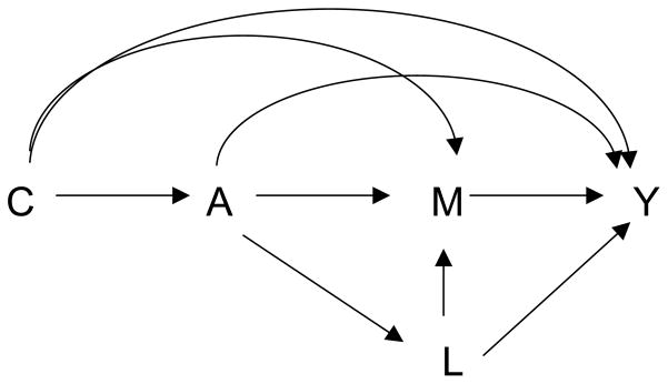
Figure 1.

Mediation with exposure A, outcome Y, mediator M, and confounders C.

Figure 2.

Mediation with a mediator-outcome confounder L that is affected by the exposure.

More general formulae involving covariates and with arbitrary exposures and mediator (rather than binary) are given in the Appendix.

The counterfactual statement of assumption (iv), Y_am ⫫ M_a^*|C, is somewhat controversial as it involves what are sometimes called “cross-world” independencies. It would hold in Figure 1 interpreted as a non-parametric structural equation model,¹⁸ but may not hold under other interpretations of causal diagrams.¹⁹ As noted above, the empirical equivalent of the four-way decomposition was (1b). As shown in the Appendix, this decomposition holds without any assumptions about confounding. However, to interpret each of the components causally does require assumptions about confounding. Assumptions (i)–(iv) above allow each of the components to be interpreted as population-average causal effects of each of the four components in the four-way individual-level counterfactual decomposition: CDE, INT_ref, INT_med, and PIE. The Appendix discusses how a slightly weaker interpretation is also valid under just assumptions (i)–(iii) alone, without requiring the more controversial assumptions (iv).

Also of interest is the fact that the controlled direct effect, CDE, requires only assumption (i) and (ii) to be identified.^1,2 This does not require the more controversial cross-world independence assumptions. The average controlled direct effect is sometimes subtracted from the average total effect to get a portion-eliminated measure E[PE] := E[TE] − E[CDE]. Whenever the total effect and the controlled direct effect can be identified, it is possible to calculate this portion-eliminated measure. Interestingly, as described further below, the four-way decomposition gives a more mechanistic interpretation of this portion-eliminated measure: the portion eliminated is the sum of the reference interaction, the mediated interaction, and the pure indirect effect (PE = INT_ref +INT_med +PIE) i.e. it is the portion due to either mediation or interaction or both. These three components cannot be empirically separated without using stronger assumptions such as (i)–(iv) above. However, whenever the total effect and the controlled direct effect can be identified (which can be done under much weaker assumptions), it is possible also to obtain also the sum of the three other components since they are simply the difference between the total effect and the controlled direct effect.

Relation to Statistical Models

Suppose that assumptions (i)–(iv) hold, that Y and M are continuous, and that the following regression models for Y and M are correctly specified:

$$E[Y\mid a,m,c]={\theta }_0+{\theta }_{1}a+{\theta }_{2}m+{\theta }_{3}am+{\theta }_4^{\prime }cE[M\mid a,c]={\beta }_0+{\beta }_{1}a+{\beta }_2^{\prime }c.$$

It is shown in the eAppendix that for exposure levels a and a^*, and setting the mediator to 0 in the controlled direct effect (see the eAppendix for other settings of mediator for the CDE), the four components are given by:

$$\begin{array}{l}E[\mathit{CDE}\mid c]={\theta }_1(a-a^{\ast })\\ E[{\mathit{INT}}_{\mathit{ref}}\mid c]={\theta }_3({\beta }_0+{\beta }_1{a}^{\ast }+{\beta }_2^{\prime }c)(a-a^{\ast })\\ E[{\mathit{INT}}_{\mathit{med}}\mid c]={\theta }_3{\beta }_1(a-a^{\ast })(a-a^{\ast })\\ E[\mathit{PIE}\mid c]=({\theta }_2{\beta }_1+{\theta }_3{\beta }_1{a}^{\ast })(a-a^{\ast })\end{array}$$

If the exposure were binary, the pure direct, reference interaction, mediated interaction, and pure indirect effects would, respectively, simply be: θ₁, ${\theta }_3({\beta }_0+{\beta }_2^{\prime }c)$}, θ₃β₁, and θ₂β₁. Standard errors for estimators of these quantities could be derived using the delta method along the lines of VanderWeele and Vansteelandt⁴ or by using bootstrapping. SAS code to implement this approach to obtain estimates and confidence intervals is provided in the eAppendix. The eAppendix likewise provides a straightforward modeling approach (with SAS code) when the mediator is binary rather than continuous.

Binary Outcomes and the Ratio Scale

The definitions of these four components has, thus far, been considered on a difference scale. Often in epidemiology, risk ratios or odds ratios are used for convenience or ease of interpretation, or to account for study design. By dividing the decomposition in (1b) by p_a=0 we can rewrite this decomposition on the ratio scale as

$$\begin{array}{l}R{R}_{a=1}-1=\kappa (R{R}_{10}-1)+\kappa (R{R}_{11}-R{R}_{10}-R{R}_{01}+1)P(M=1\mid A=0)\\ +\kappa (R{R}_{11}-R{R}_{10}-R{R}_{01}+1)\{P(M=1\mid A=1)-P(M=1\mid A=0)\}\\ +\kappa (R{R}_{01}-1)\{P(M=1\mid A=1)-P(M=1\mid A=0)\}\end{array}$$ (2)

where $R{R}_{a=1}=\frac{p_{a=1}}{p_{a=0}}$ is the relative risk for exposure A comparing A = 1 to the reference category A = 0, and $R{R}_{am}=\frac{p_{am}}{p_{00}}$ is the relative risk for comparing categories A = a, M = m to the reference category A = 0, M = 0, and where κ is a scaling factor which is given by $\kappa =\frac{p_{00}}{p_{a=0}}$. Note also that the term, (RR₁₁ − RR₁₀ − RR₀₁ + 1), is Rothman’s excess relative risk due to interaction (RERI), and is a measure of additive interaction using ratios.²⁰

The decomposition in (2) involves decomposing the excess relative risk for the exposure A, RR_a=1 − 1, into four components on the excess-relative-risk scale involving, as before, (i) the controlled direct effect of A when M = 0, (ii) a reference interaction, (iii) a mediated interaction, and (iv) a mediated main effect. Although the right-hand side of the decomposition involves a scaling factor κ, if what we are interested in is the proportion of the effect attributable to each of the components, then if out if we take any particular component and divide it by the sum of all the components, the scaling factor drops out. The proportion of the effect attributable to each of the four components is thus given by the expressions in Table 2.

Table 2.

Proportion attributable to the controlled direct effect (PA_CDE), the reference interaction (PA_INTref), the mediated interaction (PA_INTmed) and the pure indirect effect (PA_PIE) when using a ratio scale.

$$\begin{array}{l}P{A}_{\mathit{CDE}}=\frac{(R{R}_{10}-1)}{(R{R}_{10}-1)+(\mathit{RERI})P(M=1\mid A=1)+(R{R}_{01}-1)\{P(M=1\mid A=1)-P(M=1\mid A=0)\}}\\ P{A}_{\mathit{INTref}}=\frac{(\mathit{RERI})P(M=1\mid A=0)}{(R{R}_{10}-1)+(\mathit{RERI})P(M=1\mid A=1)+(R{R}_{01}-1)\{P(M=1\mid A=1)-P(M=1\mid A=0)\}}\\ P{A}_{\mathit{INTmed}}=\frac{(\mathit{RERI})\{P(M=1\mid A=1)-P(M=1\mid A=0)\}}{(R{R}_{10}-1)+(\mathit{RERI})P(M=1\mid A=1)+(R{R}_{01}-1)\{P(M=1\mid A=1)-P(M=1\mid A=0)\}}\\ P{A}_{\mathit{PIE}}=\frac{(R{R}_{01}-1)\{P(M=1\mid A=1)-P(M=1\mid A=0)\}}{(R{R}_{10}-1)+(\mathit{RERI})P(M=1\mid A=1)+(R{R}_{01}-1)\{P(M=1\mid A=1)\}-P(M=1\mid A=0)}.\end{array}$$

The four-fold proportion-attributable measures given in Table 2 allow us to estimate the proportion of the total effect attributable only to mediation (PA_PIE), due only to interaction (PA_INTref), due to both mediation and interaction (PA_INTmed), or due to neither mediation nor interaction (PA_CDE). The eAppendix provides further technical details concerning the four-way decomposition on the ratio scale and for obtaining estimates and confidence intervals using logistic regression for the outcome, along with linear regression for a continuous mediator or a second logistic regression for a binary mediator. SAS code to implement this approach is also given in the eAppendix.

Illustration

The concepts and methods described above for the four-way decomposition are illustrated here with example from genetic epidemiology. Specifically, we consider the extent to which the effect of chromosome 15q25.1 rs8034191 C alleles on lung cancer risk is due to mediation by or interaction with cigarettes smoked per day. rs8034191 C alleles are known to be associated with both smoking^26,27 and lung cancer^28–30 but there had been debate as to whether the effects on lung cancer were direct or mediated by smoking. VanderWeele et al.³¹ used methods from the causal-mediation-analysis literature to assess whether the effect was direct or indirect, and found that most of the effect was not mediated by cigarettes per day (the total indirect effect was very small and the pure direct effect was large). In large meta-analyses, Truong et al.³² found no association between the genetic variants among never-smokers, suggesting strong interaction between the variants and smoking behavior; VanderWeele et al.³¹ likewise reported statistical evidence of interaction. Here we will use the four-way decomposition to assess how much of the effect is due to each of the components.

Data are from 1836 cases and 1452 controls from a lung cancer case-control study at Massachusetts General Hospital.^31,33 As the exposure we compare 2 versus 0 C alleles, and use cigarettes per day as the mediator (the square root of this measure is used to make the measure more normally distributed). Covariates adjusted for in the analysis include sex, age, education, and smoking duration. Analyses are restricted to Caucasians. Because the outcome (lung cancer) is rare, odds ratios approximate risk ratios. A logistic regression model is fit for lung cancer on the variants, smoking, their interaction, and the covariates; and a linear regression model for smoking is fit on the variants and covariates. Confidence intervals are obtained using the delta method. Details of this modeling approach in the context of the four-way decomposition are given in the eAppendix; SAS code is also provided. Results are summarized in Table 3. The overall risk ratio comparing 2 versus 0 C alleles was 1.77 (95% confidence interval [CI]= 1.33 to 2.21) for an excess relative risk of 1.77 – 1 = 0.77 (95% CI = 0.33 to 1.21). This excess relative risk decomposes into the four components. The component due to the pure indirect effect is 0.014 (−0.01 to 0.04); the component due to the mediated interaction is 0.034 (−0.02 to 0.09); the component due to the reference interaction is 0.42 (0.11 to 0.73); and the component due to the controlled direct effect (if smoking were fixed to 0) is 0.30 (−0.19 to 0.79). The four components sum to the excess relative risk: 0.014 + 0.034 + 0.42 + 0.30 ≈ 0.77. Of these four components, the reference interaction is most substantial, highlighting the important role of interaction in this context. The overall proportion mediated (the sum of the pure indirect effect and the mediated interaction, divided by the excess relative risk) is quite small at 6% (−3% to 15%), as had been indicated in the analyses of VanderWeele et al.³¹ The overall proportion attributable to interaction (the reference interaction plus the mediated interaction, divided by the excess relative risk) is relatively substantial, 59% (9% to 109%). Mediation may play a role here (and probably does, as the variants do affect smoking and smoking affects lung cancer), but interaction, between the variants and smoking, is clearly much more important.

Table 3.

Proportions of the effect of genetic variants on lung cancer due to mediation and interaction with smoking (cigarettes per day)

Component	Excess Relative Risk	(95% CI)	Proportion Attributable	(95% CI)
CDE	0.30	(−0.19 to 0.79)	39%	(−11% to 89%)
INTref	0.42	(0.11 to 0.73)	55%	(8% to 101%)
INTmed	0.034	(−0.02 to 0.09)	4%	(−3% to 11%)
PIE	0.014	(−0.01 to 0.04)	2%	(−1% to 5%)
Total	0.77	(0.33 to 1.21)	100%

Relation to Mediation Decompositions

This section discusses the relations between the four components above and concepts from the mediation-analysis literature, and the next the relations with the interaction-analysis literature. As above, the four-fold decomposition is:

$$\begin{array}{l}{Y}_1-Y_0=(Y_{10}-Y_{00})+(Y_{11}-Y_{10}-Y_{01}+Y_{00})(M_0)\\ +(Y_{11}-Y_{10}-Y_{01}+Y_{00})(M_1-M_0)+(Y_{01}-Y_{00})(M_1-M_0).\end{array}$$

The first component, (Y₁₀ − Y₀₀), is referred to in the mediation-analysis literature as a “controlled direct effect” (CDE) of the exposure when fixing the mediator to level M = 0. Other controlled direct effects can also be considered which set M to a level other than 0; the Discussion section and Appendix consider four-way decompositions involving these alternative controlled direct effects. The fourth component in the four-way decomposition, (Y₀₁ − Y₀₀)(M₁ − M₀), which was referred to above as a “mediated main effect” is in fact equivalent to what in the mediation-analysis literature is sometimes referred to as a “pure indirect effect” (PIE). It is shown in the Appendix that:

$$\mathit{PIE}:=Y_{0M_1}-Y_{0M_0}=(Y_{01}-Y_{00})(M_1-M_0).$$

The counterfactual contrast, Y_0M1 − Y_0M0, in the mediation-analysis literature is referred to as a “pure indirect effect”¹ or as a type of “natural direct effect.”² This contrast Y_0M1 − Y_0M0 compares what would happen to the outcome if the mediator were changed from the level M₀ (the level it would be in the absence of the exposure) to M₁ (the level it would be in the presence of exposure) while in both counterfactual scenarios fixing the exposure itself to be absent. This pure indirect effect will be non-zero if and only if the exposure changes the mediator (so that M₀ and M₁ are different) and the mediator itself has an effect on the outcome even in the absence of the exposure. However, this is, in fact, the same quantity as in our decomposition above, namely (Y₀₁ − Y₀₀)(M₁ − M₀). Note that writing the pure indirect effect as (Y₀₁ − Y₀₀)(M₁ − M₀) gives a representation of the pure indirect effect that does not require nested counterfactuals of the form Y_0M1. This may be of interest as sometimes objections are made to the pure indirect effect on the grounds that nested counterfactuals of the form Y_0M1 are difficult to interpret. The third component, (Y₁₁ − Y₁₀ − Y₀₁ + Y₀₀)(M₁ − M₀), was recently considered in the mediation-analysis literature and called a “mediated interaction” (INT_med).³⁴ As discussed in the Appendix and elsewhere,³⁴ this mediated interaction can also be written as (Y_1M1 − Y_0M1 − Y_1M0 + Y_0M0). The component not yet considered is the second component, (Y₁₁ − Y₁₀ − Y₀₁ + Y₀₀)(M₀), referred to above as a “reference interaction” (INT_ref), for which there is no analog in the current literature. However, as shown in the Appendix, the sum of the first and second component does have an analog in the mediation analysis literature - it is equal to what is sometimes called the “pure direct effect” (PDE), defined as Y_1M0 − Y_0M0. This compares what would happen to the outcome in the presence versus the absence of the exposure if, in both cases, the mediator were set to whatever it would be for that individual in the absence of exposure. Expressed algebraically, we have that

$$\begin{array}{l}\mathit{PDE}:=Y_{1M_0}-Y_{0M_0}=(Y_{10}-Y_{00})+(Y_{11}-Y_{10}-Y_{01}+Y_{00})(M_0)\\ =\mathit{CDE}+{\mathit{INT}}_{\mathit{ref}}.\end{array}$$

The pure direct effect is the sum of a controlled direct effect (our first component) and the reference interaction (our second component). If in the four-way decomposition above the first two components are replaced with the pure direct effect, and the fourth component is written as the pure indirect effect, then we obtain:

$$Y_1-Y_0=\mathit{PDE}+{\mathit{INT}}_{\mathit{med}}+\mathit{PIE}.$$ (3)

In other words, the total effect can be decomposed into a pure direct effect, a pure indirect effect, and a mediated interaction. This decomposition was the three-way decomposition provided by VanderWeele³⁴ in 2013. Prior to this, a two-way decomposition was the norm in the mediation analysis literature. As discussed in the Appendix and in VanderWeele,³⁴ the sum of the mediated interaction and the pure indirect effect is equal to what in the mediation analysis literature is sometimes called a “total indirect effect” (TIE), defined as Y_1M1 − Y_1M0. Whereas the pure indirect effect, Y_0M1 − Y_0M0, compares changing the mediator from M₀ to M₁ while fixing the exposure itself to be absent, the total indirect effect, Y_1M1 − Y_1M0, compares changing the mediator from M₀ to M₁ fixing the exposure to present. With the total indirect so defined, we have TIE = PIE + INT_med i.e. (Y_1M1 − Y_1M0) = (Y_0M1 − Y_0M0) + (Y₁₁ − Y₁₀ − Y₀₁ + Y₀₀)(M₁ − M₀). It is possible then combine the mediated interaction and the pure indirect effect in the decomposition in (3) into a total indirect effect to obtain the more standard 2-way decomposition in the mediation-analysis literature:

$$Y_1-Y_0=\mathit{PDE}+\mathit{TIE}.$$ (4)

This is the decomposition used most often in the causal-inference literature when assessing direct and indirect effects; this two-way decomposition was first proposed in 1992 by Robins and Greenland¹; and it is the decomposition on which most of the software packages for causal mediation analysis have focused.^8,16 This two-way decomposition also provides the counterfactual formalization for the decompositions typically employed in the social-science literature on mediation.³⁵ However, as seen above, the pure direct effect is itself a combination of two components: a controlled direct effect and the reference interaction (PDE = CDE + INT_ref ); and the total indirect effect is a combination of two components, the pure indirect effect and the mediated interaction (TIE = PIE + INT_med). When these effects are estimated on average, a proportion-mediated measure, $\frac{E[\mathit{TIE}]}{E[TE]}$, is sometimes used; this can also be re-written as $\frac{E[\mathit{TIE}]}{E[TE]}=\frac{E[{\mathit{INT}}_{\mathit{med}}]+E[\mathit{PIE}]}{E[TE]}$.

Yet another decomposition is worth noting in the mediation analysis literature. Sometimes the mediated interaction in the decomposition in (3) is combined with the pure direct effect, rather than with the pure indirect effect, for an alternative two-way decomposition. As discussed in the Appendix and in VanderWeele,³⁴ the sum of the mediated interaction and the pure direct effect is equal to what is sometimes called a “total direct effect” (TDE),¹ defined as Y_1M1 − Y_0M1. The total and the pure direct effects are sometimes also called “natural direct effects”² and the total and the pure indirect effects are sometimes called “natural indirect effects.”² A summary of the various composite effects is given in Table 4.

Table 4.

Composite Effects

Effect	Counterfactual Definition	Composite Reliationship
Total Indirect Effect (TIE)	(Y1M1 − Y1M0)	TIE = PIE + INTmed
Pure Direct Effect (PDE)	(Y1M0 − Y0M0)	PDE = CDE + INTref
Total Direct Effect (TDE)	(Y1M1 − Y0M1)	TDE = CDE + INTref + INTmed
Portion Eliminated (PE)	(Y1 − Y0) − (Y10 − Y00)	PE = PIE + INTref + INTmed
Portion Attributable to Interaction (PAI)	(Y11 − Y10 − Y01 + Y00)(M1)	PAI = INTref + INTmed

Of interest here is that the total direct effect contains three components: the controlled direct effect, the reference interaction, and the mediated interaction. Moving from the first to the third of these components, the components involve the mediator in increasingly more substantial ways. The controlled direct effect, (Y₁₀ − Y₀₀), operates completely independent of the mediator; for this to be non-zero, the direct effect must be present even when the mediator is absent. The reference interaction, (Y₁₁ − Y₁₀ − Y₀₁ + Y₀₀)(M₀), requires the mediator to operate, but the effect does not come about by the exposure changing the mediator - it simply requires that the mediator is present even when the exposure is absent; the effect is “unmediated” in the sense that it does not operate by the exposure changing the mediator, but it requires the presence of the mediator nonetheless. The third component, the mediated interaction, (Y₁₁ − Y₁₀ − Y₀₁ + Y₀₀)(M₁ − M₀), is a type of mediated effect; it requires that the exposure change the mediator, but it is also a direct effect insofar as an interaction must also be present (the effect of the exposure is different for different levels of the mediator); the third component thus not only involves the mediator but it is a mediated effect, and a direct effect as well. For this reason, this component is sometimes combined with the pure indirect effect to obtain the total indirect effect, and sometimes combined with the pure direct effect to obtain the total direct effect.

Combining the pure direct effect and mediated interaction to get the total direct effect, TDE := Y_1M1 − Y_0M1= PDE + INT_med, gives an alternative 2-way decomposition of the total effect into the sum of the total direct effect and the pure indirect effect:

$$Y_1-Y_0=\mathit{TDE}+\mathit{PIE}.$$ (5)

This decomposition was likewise proposed by Robins and Greenland¹ in 1992. Relatively easy-to-use software is available to estimate the components of the two-way decompositions in Equations (4) and (5) on average for a population, under the assumptions described later in the paper. Note that in the decomposition in (5), the total direct effect consists of three of the four basic components (the controlled direct effect, the reference interaction, and the mediated interaction), whereas the pure indirect effect constitutes a single component. The mediated interaction is, however, arguably part of the effect that is mediated and thus, when questions of mediation are of interest, it is arguably (4), rather than (5), that is to be preferred when assessing the extent of mediation.^9,10,34 However, whether the pure indirect effect or the total indirect effect is of interest may depend upon the context.⁶

A final measure used in the mediation-analysis literature is sometimes referred to as the “portion eliminated” (PE).^1,12 As noted above, this is generally defined as the difference between the total effect and the controlled direct effect: PE := (Y₁ − Y₀) − CDE. This is the portion of the effect of the exposure that would remain if the mediator were fixed to 0. The portion eliminated may be of interest insofar as it allows one to assess how much of the effect of the exposure can be eliminated or prevented by intervening on the mediator; for this reason it is sometimes regarded as of policy interest.^1,6,12 The four-way decomposition, above, in fact shows that this portion-eliminated measure is equal to the sum of the other three components: the reference interaction, the mediated interaction, and the pure indirect effect, i.e. PE = INT_ref +INT_med+PIE; the total effect can then be written as TE = CDE + PE. The four-way decomposition provides a causal interpretation for the difference between the total effect and the controlled direct effect: it is the portion of the effect attributable to mediation, or interaction, or both. When the portion eliminated is estimated at the population level, sometimes a proportion-eliminated measure is also calculated as $\frac{E[TE]-E[\mathit{CDE}]}{E[TE]}$ which could also be rewritten as $\frac{E[{\mathit{INT}}_{\mathit{ref}}]+E[{\mathit{INT}}_{\mathit{med}}]+E[\mathit{PIE}]}{E[TE]}$. This is different from the proportion-mediated measure considered earlier, which was $\frac{E[\mathit{NIE}]}{E[TE]}=\frac{E[{\mathit{INT}}_{\mathit{med}}]+E[\mathit{PIE}]}{E[TE]}$. The proportion-eliminated includes in the numerator the reference interaction (since this part of the effect is eliminated if the mediator is removed); the proportion mediated does not include the reference interaction in the numerator (since this is not part of the mediated effect).¹²

There are thus a number of possible decompositions. However, for addressing questions of mediation, there is no need to choose between the two-way decompositions, or even the three-way decomposition; the four-way decomposition provides four components capturing all of the subtleties: the portion of the total effect that is attributable just to mediation, just to interaction, to both mediation and interaction, or to neither mediation nor interaction. The various decompositions within the context of mediation are summarized in Table 5, but the four-way decomposition here essentially provides a framework which encompasses them all.

Table 5.

Mediation Decompositions

Number of Components	Decomposition
2-Way Decompositiona	TE = TIE + PDE
2-Way Decompositionb	TE = TDE + PIE
2-Way Decompositionc	TE = CDE + PE
3-Way Decompositiond	TE = PDE + PIE + INTmed
4-Way Decompositione	TE = CDE + INTref + INTmed + PIE

^a(Y₁ − Y₀) = (Y_1M1 − Y_1M0) + (Y_1M0 − Y_0M0)

^b(Y₁ − Y₀) = (Y_1M1 − Y_0M1) + (Y_0M1 − Y_0M0)

^c(Y₁ − Y₀) = (Y₁₀ − Y₀₀) + [(Y₁ − Y₀) − (Y₁₀ − Y₀₀)]

^d(Y₁ − Y₀) = (Y_0M1 − Y_0M0) + (Y_1M0 − Y_0M0) + (Y₁₁ − Y₁₀ − Y₀₁ + Y₀₀)(M₁ − M₀)

^eY₁ − Y₀ = (Y₁₀ − Y₀₀) + (Y₁₁ − Y₁₀ − Y₀₁ + Y₀₀)(M₀) + (Y₁₁ − Y₁₀ − Y₀₁ + Y₀₀)(M₁ − M₀) + (Y₀₁ − Y₀₀)(M₁ − M₀)

Relation to Interaction Decompositions

VanderWeele and Tchetgen Tchetgen²⁴ recently considered attributing a portion of the total effect of one exposure on an outcome that is due to an interaction with a second exposure. This is related to the four-way decomposition as follows. The four-way decomposition above was expressed as:

$$Y_1-Y_0=(Y_{10}-Y_{00})+(Y_{11}-Y_{10}-Y_{01}+Y_{00})(M_0)+(Y_{11}-Y_{10}-Y_{01}+Y_{00})(M_1-M_0)+(Y_{01}-Y_{00})(M_1-M_0).$$ (1)

which can also be written as: TE = CDE + INT_ref + INT_med + PIE. Suppose now that instead of considering how much of the total effect is mediated versus direct, as in the previous section, we were interested in the portion due to interaction. In the four-way decomposition, two of the four components (the second and the third) involve an interaction. The portion due to interaction can thus be defined as their sum: PAI := INT_ref + INT_med = (Y₁₁ − Y₁₀ − Y₀₁ + Y₀₀)(M₀) + (Y₁₁ − Y₁₀ − Y₀₁ + Y₀₀)(M₁ − M₀) = (Y₁₁ − Y₁₀ − Y₀₁ + Y₀₀)(M₁), resulting in the following three-way decomposition:

$$\begin{array}{l}TE=\mathit{CDE}+\mathit{PAI}+\mathit{PIE}\\ =(Y_{10}-Y_{00})+(Y_{11}-Y_{10}-Y_{01}+Y_{00})(M_1)+(Y_{01}-Y_{00})(M_1-M_0).\end{array}$$ (6)

The total effect can be decomposed into the effect of A with M absent (CDE), a pure indirect effect (PIE), and a portion due to interaction (PAI). Consider now the empirical analog of this decomposition using the expressions in (1b). Let p_am = E[Y|A = a, M = m] and, p_a = E[Y|A = a], and p_m = E[Y|M = m]. It follows from (1b) that: (p_a=1 − p_a=0) =

$$(p_{10}-p_{00})+(p_{11}-p_{10}-p_{01}+p_{00})P(M=1\mid A=1)+(p_{01}-p_{00})\{P(M=1\mid A=1)-P(M=1\mid A=0)\}.$$ (7)

This again decomposes the average total effect of A into what is essentially the average controlled direct effect, the average portion attributable to interaction, and the average pure indirect effect. The middle component is the component due to interaction, and the proportion of the effect due to interaction could then be assessed by: (p₁₁ − p₁₀ − p₀₁ + p₀₀)P(M = 1|A = 1)/(p_a=1 − p_a=0).

In fact, the decomposition given above in (7) is that which VanderWeele and Tchetgen²⁴ used when attributing effects to interactions. Several points are worth noting. First, the decomposition in (6) and (7) for the portion attributable to interaction follows clearly from the four-way decomposition. The decomposition in (6) is the decomposition at the individual counterfactual level analogous to the empirical decomposition in (7) given by VanderWeele and Tchetgen Tchetgen.²⁴ Second, VanderWeele and Tchetgen Tchetgen considered two cases, one in which A and M were independent and one in which they are not. The decomposition in (7) was that which was proposed when A affected M. When A and M are independent, the decomposition in (7) reduces to (p_a=1 − p_a=0) = (p₁₀ − p₀₀) + (p₁₁ − p₁₀ − p₀₁ + p₀₀)P(M = 1), with a similar decomposition for the total effect of M on Y : (p_m=1 − p_m=0) = (p₀₁ − p₀₀) + (p₁₁ − p₁₀ − p₀₁ + p₀₀)P(A = 1). Similarly, on a ratio scale, when A does not affect M, the third and fourth components in Table 2 become 0, leaving $P{A}_{\mathit{CDE}}=\frac{(R{R}_{10}-1)}{(R{R}_{10}-1)+(\mathit{RERI})P(M=1)}$ and $P{A}_{\mathit{INTref}}=\frac{(\mathit{RERI})P(M=1)}{(R{R}_{10}-1)+(\mathit{RERI})P(M=1)}$, which are also the expressions given by VanderWeele and Tchetgen Tchetgen²⁴ for attributing effects to interactions on a ratio scale. When A affects M, the decomposition for the total effect of A on Y is altered, and we must use the decomposition in (7). Finally, when A does not affect Y, there is an analogous individual counterfactual-level decomposition, as (6) then reduces to: TE = (Y₁₀ − Y₀₀) + (Y₁₁ − Y₁₀ − Y₀₁ + Y₀₀)(M) since when A does not affect M, M₁ = M₀ = M. All of this also follows from the four-way decomposition, which encompasses all of the prior decompositions. These decompositions are summarized in Table 6.

Table 6.

Interaction Decompositions

Number of Components	Decomposition
2-Way Decomposition (No Mediation)a	TE = CDE + PAI
3-Way Decompositionb	TE = CDE + PAI + PIE
4-Way Decompositionc	TE = CDE + INTref + INTmed + PIE

^a(Y₁ − Y₀) = (Y₁₀ − Y₀₀) + (Y₁₁ − Y₁₀ − Y₀₁ + Y₀₀)(M)

^b(Y₁ − Y₀) = (Y₁₀ − Y₀₀) + (Y₁₁ − Y₁₀ − Y₀₁ + Y₀₀)(M₁) + (Y₀₁ − Y₀₀)(M₁ − M₀)

^c(Y₁ − Y₀) = (Y₁₀ − Y₀₀) + (Y₁₁ − Y₁₀ − Y₀₁ + Y₀₀)(M₀) + (Y₁₁ − Y₁₀ − Y₀₁ + Y₀₀)(M₁ − M₀) + (Y₀₁ − Y₀₀)(M₁ − M₀)

In the more general setting, when A affects M, it is possible to estimate the portion due to interaction on the average level using the three-way decomposition in (7). But there is no need to use only a three-way decomposition; we can instead use the four-way decomposition in (1) and the empirical expressions in (1b) to further divide the portion due to interaction into that which is due to interaction but not mediation (the reference interaction, E[INT_ref ]) and the portion due to interaction and mediation (the mediated interaction E[INT_med]). Such a four-way decomposition, in which the portion attributed to interaction is itself further divided, may shed additional insight.

Perhaps most importantly, this four-way decomposition, which helps better understand the portions of a total effect due to interaction, is exactly the same decomposition that was used above to shed insight into what portions of the total effect were mediated and which portions were direct. The same four-way decomposition was useful in assessing both mediation and interaction. The same four components are used in assessing mediation and interaction, but the components are combined in different ways to assess these different phenomena. The four-way decomposition itself provides a unification of mediation and interaction. The four-fold decomposition underlies the various more specific decompositions in assessing both mediation and interaction. As illustrated in Figure 3, the four components form the backbone of both the various mediation decompositions (Figures 3–5) and the interaction decomposition (Figure 3). Once, again, however, the greatest insight is gained when the four-fold approach is used to assess simultaneously the portions of the total effect that are due only to mediation, only to interaction, to both mediation and interaction, and to neither mediation nor interaction.

Figure 3.

The four-fold decomposition encompasses both decompositions for mediation and interaction. For interaction, the reference interaction (INT_ref) and the mediated interaction (INT_med) combine to the portion attributable to interaction (PAI). The portion attributable to interaction (PAI) combine with the controlled direct effect (CDE) and the pure indirect effect (PIE) to give the total effect (TE). For mediation, the controlled direct effect and the reference interaction (INT_ref) combine to give the pure direct effect (PDE); the pure indirect effect (PIE) combines with the mediated interaction (INT_med) to give the total indirect effect (TIE); and the pure direct effect (PDE) combines with total indirect effect (TIE) to give the total effect (TE).

Figure 5.

As an alternative mediation decomposition, the difference between the total effect (TE) and the controlled direct effect (PE) is sometimes called the portion eliminated (PE) and it is equal to the sum of the reference interaction (INT_ref), the mediated interaction (INT_med), and the pure indirect effect (PIE).

Discussion

A four-way decomposition has been given here that encompasses and unites previous decompositions in the literature, both concerning mediation and concerning interaction. The results provide a mechanistic interpretation of the difference between a total effect and a controlled direct effect; this contrast has been used to assess policy implications, and it is more easily identified than many other causal quantities concerning mediation; the results here show that it also has a mechanistic interpretation as well. The four-way decomposition can be carried out on a difference scale and on a ratio scale; its components can be related to standard statistical models; and software code is provided in the eAppendix to estimate the various components of the decomposition using regression models. In addition to reporting the four components, an investigator can also easily report the overall proportion attributable to interaction, the overall proportion mediated, and the proportion of the effect that would be eliminated if the mediator were removed. As seen in the empirical example in genetic epidemiology, this approach can shed considerable insight into the relationships between an exposure and a mediator with an outcome, and into the role of both mediation and interaction in these relationships.

The focus here has been on a binary exposure and binary mediator, with the controlled direct effect being that in which the mediator is fixed to be absent. More general results are given in the Appendix, and the approach in fact applies to arbitrary exposures and mediators. Moreover, instead of focusing on a controlled direct effect with the mediator absent, one can consider controlled direct effects that fix the mediator to some other level, m^*. Similar four-way decompositions can be carried out wherein the first component is the controlled direct effect with the mediator fixed to level m^*. When this is done, the reference interaction term changes because, with the mediator fixed to m^* (rather than 0), the controlled direct effect picks up some of the effect of the interaction between the exposure and the mediator. With a controlled direct effect in which the mediator is fixed to m^*, the interpretation of the reference interaction is then the portion of the effect due to the interaction between the exposure and the mediator that is not mediated, and also not captured by the controlled direct effect. Again, the results in the Appendix cover more general settings and will thus likely be of use in a variety of contexts. The code in the eAppendix likewise provides practical and relatively easy-to-use software tools to implement the approaches here in a wide range of settings.

The central limitations of the approach developed here is the strong assumptions about confounding. These assumptions are, however, the same assumptions to those made in the literature on mediation that focuses only on simpler decompositions. Future research could examine the robustness of each of the four components to confounding and measurement error. For example, recent work indicates that interaction terms may be more robust to confounding,³⁶ but that interaction terms when the two exposures are correlated may be particularly sensitive to measurement error^37,38; different components may be robust to different forms of bias. Future work could also extend existing sensitivity-analysis techniques for mediation and interaction^7,8,36–38 to each of the four components.

Prior work on mediation within the counterfactual framework has accommodated potential interaction. The present approach clarifies the role of interaction, and its separate contribution beyond mediation, and unites, within a single framework, the phenomena of mediation and interaction.

Figure 4.

As an alternative mediation decomposition, the controlled direct effect and the reference interaction (INT_ref) combine to give the pure direct effect (PDE); the pure direct effect (PDE) and the mediated interaction (INT_med) combine to give the total direct effect (TDE); and the total direct effect (TDE) and the pure indirect effect (PIE) combine to give the total effect (TE).

Appendix

In the Appendix we will no longer restrict attention to binary exposure and mediator and will consider an arbitrary exposure and mediator. We will assume we are comparing two exposure levels a and a^*. We give the general four-way decomposition result in Proposition 1.

Proposition 1

For any level m^* of M we have Y_a − Y_a^*

$$\begin{array}{l}=(Y_{a{m}^{\ast }}-Y_{a^{\ast }{m}^{\ast }})+{\sum }_m(Y_{am}-Y_{a^{\ast }m}-Y_{a{m}^{\ast }}+Y_{a^{\ast }{m}^{\ast }})1(M_{a^{\ast }}=m)\\ +{\sum }_m(Y_{am}-Y_{a^{\ast }m})\{1(M_a=m)-1(M_{a^{\ast }}=m)\}+(Y_{a^{\ast }{M}_a}-Y_{a^{\ast }{M}_{a^{\ast }}})\end{array}$$

Proof

We have that Y_a − Y_a^*

$$\begin{array}{l}=Y_{a{M}_a}-Y_{a^{\ast }{M}_{a^{\ast }}}\\ =(Y_{a{M}_a}-Y_{a^{\ast }{M}_a})+(Y_{a^{\ast }{M}_a}-Y_{a^{\ast }{M}_{a^{\ast }}})\\ =(Y_{a{M}_{a^{\ast }}}-Y_{a^{\ast }{M}_{a^{\ast }}})+(Y_{a^{\ast }{M}_a}-Y_{a^{\ast }{M}_{a^{\ast }}})+(Y_{a{M}_a}-Y_{a^{\ast }{M}_a}-Y_{a{M}_{a^{\ast }}}+Y_{a^{\ast }{M}_{a^{\ast }}})\\ =(Y_{a{m}^{\ast }}-Y_{a^{\ast }{m}^{\ast }})+\{(Y_{a{M}_{a^{\ast }}}-Y_{a^{\ast }{M}_{a^{\ast }}})-(Y_{a{m}^{\ast }}-Y_{a^{\ast }{m}^{\ast }})\}\\ +(Y_{a{M}_a}-Y_{a^{\ast }{M}_a}-Y_{a{M}_{a^{\ast }}}+Y_{a^{\ast }{M}_{a^{\ast }}})+(Y_{a^{\ast }{M}_a}-Y_{a^{\ast }{M}_{a^{\ast }}})\\ =(Y_{a{m}^{\ast }}-Y_{a^{\ast }{m}^{\ast }})+{\sum }_m\{(Y_{am}-Y_{a^{\ast }m})-(Y_{a{m}^{\ast }}-Y_{a^{\ast }{m}^{\ast }})\}1(M_{a^{\ast }}=m)\\ +{\sum }_m\{(Y_{am}-Y_{a^{\ast }m})1(M_a=m)-(Y_{am}-Y_{a^{\ast }m})1(M_{a^{\ast }}=m)\}+(Y_{a^{\ast }{M}_a}-Y_{a^{\ast }{M}_{a^{\ast }}})\\ =(Y_{a{m}^{\ast }}-Y_{a^{\ast }{m}^{\ast }})+{\sum }_m(Y_{am}-Y_{a^{\ast }m}-Y_{a{m}^{\ast }}+Y_{a^{\ast }{m}^{\ast }})1(M_{a^{\ast }}=m)\\ +{\sum }_m(Y_{am}-Y_{a^{\ast }m})\{1(M_a=m)-1(M_{a^{\ast }}=m)\}+(Y_{a^{\ast }{M}_a}-Y_{a^{\ast }{M}_{a^{\ast }}}).\end{array}$$

This completes the proof.

The four components of the decomposition in general form are thus

$$\begin{array}{l}\mathit{CDE}(m^{\ast }):=(Y_{a{m}^{\ast }}-Y_{a^{\ast }{m}^{\ast }})\\ {\mathit{INT}}_{\mathit{ref}}(m^{\ast }):={\sum }_m(Y_{am}-Y_{a^{\ast }m}-Y_{a{m}^{\ast }}+Y_{a^{\ast }{m}^{\ast }})1(M_{a^{\ast }}=m)\\ {\mathit{INT}}_{\mathit{med}}:={\sum }_m(Y_{am}-Y_{a^{\ast }m})\{1(M_a=m)-1(M_{a^{\ast }}=m)\}\\ \mathit{PIE}:=(Y_{a^{\ast }{M}_a}-Y_{a^{\ast }{M}_{a^{\ast }}}).\end{array}$$

Note we can also rewrite INT_med = Σ_m(Y_am − Y_a^*m − Y_am^* + Y_a^*m^*){1(M_a = m) − 1(M_a^* = m)} and we can rewrite PIE = Σ_m(Y_a^*m − Y_a^*m^*){1(M_a = m) − 1(M_a^* = m)}. Doing so with binary A and M and setting a = 1, a^* = 0, m^* = 0 gives us the decomposition in (1) in the text:

$$Y_1-Y_0=(Y_{10}-Y_{00})+(Y_{11}-Y_{10}-Y_{01}+Y_{00})(M_0)+(Y_{11}-Y_{10}-Y_{01}+Y_{00})(M_1-M_0)+(Y_{01}-Y_{00})(M_1-M_0).$$ (1)

The decomposition also has an empirical analogue given in the next Proposition.

Proposition 2

For any level m^* of M we have E[Y|a, c] − E[Y|a^*, c] =

$$\begin{array}{l}=\{E[Y\mid a,m^{\ast },c]-E[Y\mid a^{\ast },m^{\ast },c]\}\\ +\int \{E[Y\mid a,m,c]-E[Y\mid a^{\ast },m,c]-E[Y\mid a,m^{\ast },c]+E[Y\mid a^{\ast },m^{\ast },c]\}dP(m\mid a^{\ast },c)\\ +\int \{E[Y\mid a,m,c]-E[Y\mid a^{\ast },m,c]\}\{dP(m\mid a,c)-dP(m\mid a^{\ast },c)\}\\ +\int E[Y\mid a^{\ast },m,c]\{dP(m\mid a,c)-dP(m\mid a^{\ast },c)\}.\end{array}$$

Proof

We have that E[Y|a, c] − E[Y|a^*, c]

$$\begin{array}{l}=E[Y\mid a,m^{\ast },c]-E[Y\mid a^{\ast },m^{\ast },c]+\{E[Y\mid a,c]-E[Y\mid a,m^{\ast },c]\}-\{E[Y\mid a^{\ast },c]-E[Y\mid a^{\ast },m^{\ast },c]\}\\ =E[Y\mid a,m^{\ast },c]-E[Y\mid a^{\ast },m^{\ast },c]+\int \{E[Y\mid a,m,c]-E[Y\mid a,m^{\ast },c]\}dP(m\mid a,c)\\ -\int \{E[Y\mid a^{\ast },m,c]-E[Y\mid a^{\ast },m^{\ast },c]\}dP(m\mid a^{\ast },c)\\ =\{E[Y\mid a,m^{\ast },c]-E[Y\mid a^{\ast },m^{\ast },c]\}\\ +\int \{E[Y\mid a,m,c]-E[Y\mid a^{\ast },m,c]\}-\{E[Y\mid a,m^{\ast },c]-E[Y\mid a^{\ast },m^{\ast },c]\}dP(m\mid a,c)\\ +\int \{E[Y\mid a^{\ast },m,c]-E[Y\mid a^{\ast },m^{\ast },c]\}\{dP(m\mid a,c)-dP(m\mid a^{\ast },c)\}\\ =\{E[Y\mid a,m^{\ast },c]-E[Y\mid a^{\ast },m^{\ast },c]\}\\ +\int \{E[Y\mid a,m,c]-E[Y\mid a^{\ast },m,c]\}-\{E[Y\mid a,m^{\ast },c]-E[Y\mid a^{\ast },m^{\ast },c]\}dP(m\mid a^{\ast },c)\\ +\int \{E[Y\mid a,m,c]-E[Y\mid a^{\ast },m,c]\}-\{E[Y\mid a,m^{\ast },c]-E[Y\mid a^{\ast },m^{\ast },c]\}\{dP(m\mid a,c)-dP(m\mid a^{\ast },c)\}\\ +\int \{E[Y\mid a^{\ast },m,c]-E[Y\mid a^{\ast },m^{\ast },c]\}\{dP(m\mid a,c)\}-dP(m\mid a^{\ast },c)\}.\\ =\{E[Y\mid a,m^{\ast },c]-E[Y\mid a^{\ast },m^{\ast },c]\}\\ +\int \{E[Y\mid a,m,c]-E[Y\mid a^{\ast },m,c]-E[Y\mid a,m^{\ast },c]+E[Y\mid a^{\ast },m^{\ast },c]\}dP(m\mid a^{\ast },c)\\ +\int \{E[Y\mid a,m,c]-E[Y\mid a^{\ast },m,c]\}\{dP(m\mid a,c)-dP(m\mid a^{\ast },c)\}\\ +\int E[Y\mid a^{\ast },m,c]\{dP(m\mid a,c)-dP(m\mid a^{\ast },c)\}.\end{array}$$

Note we can also rewrite the third term as ∫ {E[Y|a, m, c] − E[Y|a^*, m, c]} − {E[Y|a, m^*, c] − E[Y|a^*, m^*, c]}{dP(m|a, c) − dP(m|a^*, c)} and the fourth term as ∫ {E[Y|a^*, m, c] − E[Y|a^*, m^*, c]}{dP(m|a, c) − dP(m|a^*, c)}. Doing so with binary A and M, and setting a = 1, a^* = 0, m^* = 0 gives decomposition (1b) in the text:

$$\begin{array}{l}{p}_{a=1}-p_{a=0}=(p_{10}-p_{00})+(p_{11}-p_{10}-p_{01}+p_{00})P(M=1\mid A=0)\\ +(p_{11}-p_{10}-p_{01}+p_{00})\{P(M=1\mid A=1)-P(M=1\mid A=0)\}\\ +(p_{01}-p_{00})\{P(M=1\mid A=1)-P(M=1\mid A=0)\}\end{array}$$ (1b)

Note the decomposition in Proposition 2 is a property of the expectations and probabilities. It does not require confounding assumptions. However, to interpret the components as causal effects, confounding assumptions are required. We will begin our discussion of confounding by first considering non-parametric structural equations.¹⁸ Consider the following four confounding assumptions: (i) the effect the exposure A on the outcome Y is unconfounded conditional on C; (ii) the effect the mediator M on the outcome Y is unconfounded conditional on (C, A); (iii) the effect the exposure A on the mediator M is unconfounded conditional on C; and (iv) none of the mediator-outcome confounders are themselves affected by the exposure. If we let X ⫫ Y|Z denote that X is independent of Y conditional on Z, then these four assumptions stated formally in terms of counterfactual independence are: (i) Y_am ⫫ A|C, (ii) Y_am ⫫ M|{A, C}, (iii) M_a ⫫ A|C, and (iv) Y_am ⫫ M_a^*|C.

Proposition 3

Under assumptions (i)–(iv) we have:

$$\begin{array}{l}E[\mathit{CDE}(m^{\ast })\mid c]=\{E[Y\mid a,m^{\ast },c]-E[Y\mid a^{\ast },m^{\ast },c]\}\\ E[{\mathit{INT}}_{\mathit{ref}}(m^{\ast })\mid c]=\int \{E[Y\mid a,m,c]-E[Y\mid a^{\ast },m,c]-E[Y\mid a,m^{\ast },c]+E[Y\mid a^{\ast },m^{\ast },c]dP(m\mid a^{\ast },c)\\ E[{\mathit{INT}}_{\mathit{med}}\mid c]=\int \{E[Y\mid a,m,c]-E[Y\mid a^{\ast },m,c]\}\{dP(m\mid a,c)-dP(m\mid a^{\ast },c)\}\\ E[\mathit{PIE}\mid c]=\int E[Y\mid a^{\ast },m,c]\{dP(m\mid a,c)-dP(m\mid a^{\ast },c)\}.\end{array}$$

Proof

The first equality is established by Robins,³⁹ the fourth by Pearl,² and the third by VanderWeele.³⁴ For the second equality we have E[INT_ref (m^*)|c]

$$\begin{array}{l}=E\left[{\sum }_m(Y_{am}-Y_{a^{\ast }m}-Y_{a{m}^{\ast }}+Y_{a^{\ast }{m}^{\ast }})1(M_{a^{\ast }}=m)\mid c\right]\\ ={\int }_{m}E[Y_{am}-Y_{a^{\ast }m}-Y_{a{m}^{\ast }}+Y_{a^{\ast }{m}^{\ast }}\mid c]dP(M_{a^{\ast }}=m\mid c)\\ ={\int }_m\{E[Y_{am}\mid c]-E[Y_{a^{\ast }m}\mid c]-E[Y_{a{m}^{\ast }}\mid c]+E[Y_{a^{\ast }{m}^{\ast }}\mid c]\}dP(M_{a^{\ast }}=m\mid c)\\ ={\int }_m\{E[Y_{am}\mid a,m,c]-E[Y_{a^{\ast }m}\mid a^{\ast },m,c]-E[Y_{a{m}^{\ast }}\mid a,m^{\ast },c]+E[Y_{a^{\ast }{m}^{\ast }}\mid a^{\ast },m^{\ast },c]\}dP(M_{a^{\ast }}=m\mid a^{\ast },c)\\ ={\int }_m\{E[Y\mid a,m,c]-E[Y\mid a^{\ast },m,c]-E[Y\mid a,m^{\ast },c]+E[Y\mid a^{\ast },m^{\ast },c]\}dP(M=m\mid a^{\ast },c)\end{array}$$

where the second equality follows by assumption (iv) and the fourth by assumptions (i)–(iii). In fact, the other three equalities in Proposition 3 can be established in much the same way. This completes the proof.

We can also interpret the terms in the decomposition in Proposition 2 causally under assumptions (i)–(iii) alone, though the causal interpretation is slightly weaker.

Proposition 4

Under assumptions (i)–(iii) we have:

$$\begin{array}{l}\{E[Y\mid a,m^{\ast },c]-E[Y\mid a^{\ast },m^{\ast },c]\}=E[Y_{a{m}^{\ast }}-Y_{a^{\ast }{m}^{\ast }}\mid c]\\ \int \{E[Y\mid a,m,c]-E[Y\mid a^{\ast },m,c]-E[Y\mid a,m^{\ast },c]+E[Y\mid a^{\ast },m^{\ast },c]\}dP(m\mid a^{\ast },c)\\ =\int E[Y_{am}-Y_{a^{\ast }m}-Y_{a{m}^{\ast }}+Y_{a^{\ast }{m}^{\ast }}\mid c]dP(M_{a^{\ast }}\mid c)\\ \int \{E[Y\mid a,m,c]-E[Y\mid a^{\ast },m,c]\}\{dP(m\mid a,c)-dP(m\mid a^{\ast },c)\}\\ =\int E[Y_{am}-Y_{a^{\ast }m}\mid c]\{dP(M_a\mid c)-dP(M_{a^{\ast }}\mid c)\\ \int E[Y\mid a^{\ast },m,c]\{dP(m\mid a,c)-dP(m\mid a^{\ast },c)\}=\int E[Y_{a^{\ast }m}\mid c]\{dP(M_a\mid c)-dP(M_{a^{\ast }}\mid c)\}.\end{array}$$

Proof

The first equality is established by Robins,³⁹ the second in the final four lines of the proof of Proportion 3 above, the third in VanderWeele,³⁴ and the fourth, using slightly different notation, by Didelez et al.⁴⁰ This completes the proof.

Note we can also rewrite the right side of the third equality as ∫ {E[Y_am − Y_a^*m|c] − E[Y_am^* − Y_a^*m^*|c]}{dP(M_a|c)−dP(M_a^*|c) and the right side of the fourth equality as ∫ {E[Y_a^*m − Y_a^*m^*}c]}{dP(M_a|c)− dP(M_a^*|c)}. The right side of the equalities in Proposition 4 are causal quantities, but rather than directly taking population averages of the four components of the decomposition, the effects of A and M on Y are integrated over the distribution of M under different exposure settings. As discussed further in the eAppendix, these effects can be interpreted as randomized interventional analogs of the four components of the decomposition. They require only assumptions (i)–(iii) for identification (i.e. they do not require the more controversial cross-world independence assumption (iv)), but the causal interpretation of these randomized interventional analogues is somewhat weaker.

Finally, we note that some earlier literature on interaction with binary exposures made use of different response types where individuals were classified according to their joint counterfactual outcomes (Y₀₀, Y₀₁, Y₁₀, Y₁₁). Under the response-type classification for mediation given by Hafeman and VanderWeele⁴¹ (in which it is assumed that the monotonicity assumption that Y_am is non-decreasing in a and in m holds), the four components of the four-decomposition could be written as CDE(0) = Y₍₂₎+ Y₍₄₎, INT_ref (0) = M₍₁₎(Y₍₈₎ − Y₍₂₎), INT_med = M₍₂₎(Y₍₈₎ − Y₍₂₎), and PIE = M₍₂₎(Y₍₂₎ + Y₍₆₎) where M₍₁₎ is a binary indicator such that M₍₁₎ = 1 if M₀ = M₁ = 1 and M₍₁₎ = 0 otherwise; M₍₂₎ is a binary indicator such that M₍₂₎ = 1 if M₀ = 0, M₁ = 1 and M₍₂₎ = 0 otherwise; Y₍₂₎ is a binary indicator such that Y₍₂₎ = 1 if (Y₀₀ = 0, Y₀₁ = 1, Y₁₀ = 1, Y₁₁ = 1) and Y₍₂₎ = 0 otherwise; Y₍₄₎ is a binary indicator such that Y₍₄₎ = 1 if (Y₀₀ = 0, Y₀₁ = 0, Y₁₀ = 1, Y₁₁ = 1) and Y₍₄₎ = 0 otherwise; Y₍₆₎ is a binary indicator such that Y₍₆₎ = 1 if (Y₀₀ = 0, Y₀₁ = 1, Y₁₀ = 0, Y₁₁ = 1) and Y₍₆₎ = 0 otherwise; and Y₍₈₎ is a binary indicator such that Y₍₈₎ = 1 if (Y₀₀ = 0, Y₀₁ = 1, Y₁₀ = 1, Y₁₁ = 1) and Y₍₈₎ = 0 otherwise.

References

- 1.Robins JM, Greenland S. Identifiability and exchangeability for direct and indirect effects. Epidemiology. 1992;3:143–155. doi: 10.1097/00001648-199203000-00013. [DOI] [PubMed] [Google Scholar]
- 2.Pearl J. Direct and indirect effects. Proceedings of the Seventeenth Conference on Uncertainty and Artificial Intelligence; San Francisco: Morgan Kaufmann; 2001. pp. 411–420. [Google Scholar]
- 3.Avin C, Shpitser I, Pearl J. Identifiability of path-specific effects. Proceedings of the International Joint Conferences on Artificial Intelligence; 2005. pp. 357–363. [Google Scholar]
- 4.VanderWeele TJ, Vansteelandt S. Conceptual issues concerning mediation, interventions and composition. Statistics and Its Interface - Special Issue on Mental Health and Social Behavioral Science. 2009;2:457–468. [Google Scholar]
- 5.VanderWeele TJ, Vansteelandt S. Odds ratios for mediation analysis with a dichotomous outcome. American Journal of Epidemiology. 2010;172:1339–1348. doi: 10.1093/aje/kwq332. [DOI] [PMC free article] [PubMed] [Google Scholar]
- 6.Hafeman D, Schwartz S. Opening the black box: a motivation for the assessment of mediation. International Journal of Epidemiology. 2009;38:838–845. doi: 10.1093/ije/dyn372. [DOI] [PubMed] [Google Scholar]
- 7.VanderWeele TJ. Bias formulas for sensitivity analysis for direct and indirect effects. Epidemiology. 2010;21:540–551. doi: 10.1097/EDE.0b013e3181df191c. [DOI] [PMC free article] [PubMed] [Google Scholar]
- 8.Imai K, Keele L, Tingley D. A general approach to causal mediation analysis. Psychological Methods. 2010;15:309–334. doi: 10.1037/a0020761. [DOI] [PubMed] [Google Scholar]
- 9.VanderWeele TJ. Subtleties of explanatory language: what is meant by “mediation”? European Journal of Epidemiology. 2011;26:343–346. doi: 10.1007/s10654-011-9588-z. [DOI] [PMC free article] [PubMed] [Google Scholar]
- 10.Suzuki E, Yamamoto E, Tsuda T. Identification of operating mediation and mechanism in the sufficient-component cause framework. European Journal of Epidemiology. 2011;26:347–57. doi: 10.1007/s10654-011-9568-3. [DOI] [PubMed] [Google Scholar]
- 11.VanderWeele TJ. Causal mediation analysis with survival data. Epidemiology. 2011;22:582–585. doi: 10.1097/EDE.0b013e31821db37e. [DOI] [PMC free article] [PubMed] [Google Scholar]
- 12.VanderWeele TJ. Policy-relevant proportions for direct effects. Epidemiology. 2013;24:175–176. doi: 10.1097/EDE.0b013e3182781410. [DOI] [PMC free article] [PubMed] [Google Scholar]
- 13.Lange T, Hansen JV. Direct and indirect effects in a survival context. Epidemiology. 2011;22:575–581. doi: 10.1097/EDE.0b013e31821c680c. [DOI] [PubMed] [Google Scholar]
- 14.Tchetgen Tchetgen EJ. On causal mediation analysis with a survival outcome. International Journal of Biostatistics. 2011;7:Article 33, 1–38. doi: 10.2202/1557-4679.1351. [DOI] [PMC free article] [PubMed] [Google Scholar]
- 15.Tchetgen Tchetgen EJ, Shpitser I. Semiparametric theory for causal mediation analysis: efficiency bounds, multiple robustness, and sensitivity analysis. Annals of Statistics. 2012;40(3):1816–1845. doi: 10.1214/12-AOS990. [DOI] [PMC free article] [PubMed] [Google Scholar]
- 16.Valeri L, VanderWeele TJ. Mediation analysis allowing for exposure-mediator interactions and causal interpretation: theoretical assumptions and implementation with SAS and SPSS macros. Psychological Methods. 2013;18:137–150. doi: 10.1037/a0031034. [DOI] [PMC free article] [PubMed] [Google Scholar]
- 17.Robins JM. Semantics of causal DAG models and the identification of direct and indirect effects. In: Green P, Hjort NL, Richardson S, editors. Highly Structured Stochastic Systems. Oxford University Press; New York: 2003. pp. 70–81. [Google Scholar]
- 18.Pearl J. Causality: Models, Reasoning, and Inference. 2. Cambridge: Cambridge University Press; 2009. [Google Scholar]
- 19.Robins JM, Richardson TS. Alternative graphical causal models and the identification of direct effects. In: Shrout P, editor. Causality and Psychopathology: Finding the Determinants of Disorders and Their Cures. Oxford University Press; 2010. [Google Scholar]
- 20.Rothman KJ. Modern Epidemiology. 1. Little, Brown and Company; Boston, MA: 1986. [Google Scholar]
- 21.Hosmer DW, Lemeshow S. Confidence interval estimation of interaction. Epidemiology. 1992;3:452–56. doi: 10.1097/00001648-199209000-00012. [DOI] [PubMed] [Google Scholar]
- 22.Rothman KJ, Greenland S, Lash TL. Modern Epidemiology. 3. chapter 5. Philadelphia: Lippincott Williams and Wilkins; 2008. Concepts of interaction. [Google Scholar]
- 23.VanderWeele TJ. Reconsidering the denominator of the attributable proportion for interaction. European Journal of Epidemiology. 2013;28:779–784. doi: 10.1007/s10654-013-9843-6. [DOI] [PMC free article] [PubMed] [Google Scholar]
- 24.VanderWeele TJ, Tchetgen Tchetgen EJ. Attributing effects to interactions. Epidemiology. doi: 10.1097/EDE.0000000000000096. in press. [DOI] [PMC free article] [PubMed] [Google Scholar]
- 25.VanderWeele TJ. Concerning the consistency assumption in causal inference. Epidemiology. 2009;20:880–883. doi: 10.1097/EDE.0b013e3181bd5638. [DOI] [PubMed] [Google Scholar]
- 26.Saccone SF, Hinrichs AL, Saccone NL, et al. Cholinergic nicotinic receptor genes implicated in a nicotine dependence association study targeting 348 candidate genes with 3713 SNPs. Hum Mol Genet. 2007;16(1):36–49. doi: 10.1093/hmg/ddl438. [DOI] [PMC free article] [PubMed] [Google Scholar]
- 27.Spitz MR, Amos CI, Dong Q, et al. The CHRNA5-A3 region on chromosome 15q24-25.1 is a risk factor both for nicotine dependence and for lung cancer. J Natl Cancer Inst. 2008;100(21):1552–1556. doi: 10.1093/jnci/djn363. [DOI] [PMC free article] [PubMed] [Google Scholar]
- 28.Hung RJ, McKay JD, Gaborieau V, et al. A susceptibility locus for lung cancer maps to nicotinic acetylcholine receptor subunit genes on 15q25. Nature. 2008;452(7187):633–637. doi: 10.1038/nature06885. [DOI] [PubMed] [Google Scholar]
- 29.Amos CI, Wu X, Broderick P, et al. Genome-wide association scan of tag SNPs identifies a susceptibility locus for lung cancer at 15q25.1. Nat Genet. 2008;40(5):616–622. doi: 10.1038/ng.109. [DOI] [PMC free article] [PubMed] [Google Scholar]
- 30.Thorgeirsson TE, Geller F, Sulem P, et al. A variant associated with nicotine dependence, lung cancer and peripheral arterial disease. Nature. 2008;452(7187):638–642. doi: 10.1038/nature06846. [DOI] [PMC free article] [PubMed] [Google Scholar]
- 31.VanderWeele TJ, Asomaning K, Tchetgen Tchetgen EJ, Han Y, Spitz MR, Shete S, Wu X, Gaborieau V, Wang Y, McLaughlin J, Hung RJ, Brennan P, Amos CI, Christiani DC, Lin X. Genetic variants on 15q25. 1, smoking and lung cancer: an assessment of mediation and interaction. American Journal of Epidemiology. 2012;175:1013–1020. doi: 10.1093/aje/kwr467. [DOI] [PMC free article] [PubMed] [Google Scholar]
- 32.Truong T, Hung RJ, Amos CI, et al. Replication of lung cancer susceptibility loci at chromosomes 15q25, 5p15, and 6p21: a pooled analysis from the International Lung Cancer Consortium. J Natl Cancer Inst. 2010;102(13):959–971. doi: 10.1093/jnci/djq178. [DOI] [PMC free article] [PubMed] [Google Scholar]
- 33.Miller DP, Liu G, De Vivo I, et al. Combinations of the variant genotypes of GSTP1, GSTM1, and p53 are associated with an increased lung cancer risk. Cancer Res. 2002;62(10):2819–2823. [PubMed] [Google Scholar]
- 34.VanderWeele TJ. A three-way decomposition of a total effect into direct, indirect, and interactive effects. Epidemiology. 2013;24:224–232. doi: 10.1097/EDE.0b013e318281a64e. [DOI] [PMC free article] [PubMed] [Google Scholar]
- 35.MacKinnon DP. Introduction to Statistical Mediation Analysis. New York: Erlbaum; 2008. [Google Scholar]
- 36.VanderWeele TJ, Mukherjee B, Chen J. Sensitivity analysis for interactions under unmeasured confounding. Statistics in Medicine. 2012;31:2552–2564. doi: 10.1002/sim.4354. [DOI] [PMC free article] [PubMed] [Google Scholar]
- 37.Valeri L, Lin X, VanderWeele TJ. Mediation analysis when a continuous mediator is measured with error and the outcome follows a generalized linear model. Statistics in Medicine. doi: 10.1002/sim.6295. [DOI] [PMC free article] [PubMed] [Google Scholar]
- 38.Valeri L, Vander Weele TJ. The estimation of direct and indirect causal effects in the presence of a misclassified binary mediator. Biostatistics. doi: 10.1093/biostatistics/kxu007. in press. [DOI] [PMC free article] [PubMed] [Google Scholar]
- 39.Robins JM. A new approach to causal inference in mortality studies with sustained exposure period - application to control of the healthy worker survivor effect. Mathematical Modelling. 1986;7:1393–1512. [Google Scholar]
- 40.Didelez V, Dawid AP, Geneletti S. Direct and indirect effects of sequential treatments. Proceedings of the Twenty-Second Conference on Uncertainty in Artificial Intelligence; Arlington, VA: AUAI Press; 2006. pp. 138–146. [Google Scholar]
Associated Data
This section collects any data citations, data availability statements, or supplementary materials included in this article.