Correction of Gradient Nonlinearity Artifacts in Prospective Motion Correction for 7T MRI

Abstract

Purpose

To demonstrate the effect of gradient nonlinearity and develop a method for correction of gradient non-linearity artifacts in prospective motion correction (Mo-Co).

Methods

Non-linear gradients can induce geometric distortions in MRI, leading to pixel shifts with errors of up to several millimeters, thereby interfering with precise localization of anatomical structures. Prospective Mo-Co has been extended by conventional gradient warp correction applied to individual phase encoding steps/groups during the reconstruction. The gradient-related displacements are approximated using Spherical Harmonic (SPH) functions. In addition, the combination of this method with a retrospective correction of the changes in the coil sensitivity profiles relative to the object (augmented SENSE) was evaluated in simulation and experimental data.

Results

Prospective Mo-Co under gradient fields and coils sensitivity inconsistencies results in residual blurring, spatial distortion, and coil sensitivity mismatch artifacts. These errors can be considerably mitigated by the proposed method. High image quality with very little remaining artifacts was achieved after a few iterations. The relative image errors decreased from 25.7% to below 17.3% after 10 iterations.

Conclusion

The combined correction of gradient non-linearity and sensitivity map variation leads to a pronounced reduction of residual motion artifacts in prospectively motion-corrected data.

Introduction

Numerous motion correction techniques have been presented. They can be categorized into methods for retrospective and prospective corrections based on motion information that originates from MR-data, i.e. navigator echoes (1) and self-navigated (2) or from external motion detection devices (3). When motion occurred only infrequently during an examination, the image quality can be improved after either the corrupted signals were rejected or replaced by resampled signals (2,4). Retrospective correction (5,6) was applied in the image reconstruction process by reversing the motion effects on the corrupted signals. As a way of preventing inconsistent k-space data, real-time prospective correction (7-9) has been proposed with continuous or repeated position determination followed by gradient and RF adjustment immediately before each excitation to result in data as if no movement had occurred. Not only can spin history effects be avoided but also no extra imaging time is required when an external tracking system is used (9).

With large motion, even if prospective motion tracking is perfectly accurate and delays are minimal, the acquired images can be contaminated by residual artifacts that cannot be corrected for with rigid body pose updates alone (10). The acquired raw data of the imaged object can become inconsistent if, despite prospective correction of the object pose, the MR-image of the object changes. The main reasons for such image variations with object pose are intensity variations due to coil sensitivities that change relative to the object (11-13) and spatial distortions, including object-dependent chemical shift and susceptibility changes, hardware-related sources such as static field inhomogeneity and gradient field non-linearity that deform the reconstructed image depending on the object pose. These issues need to be addressed to further improve image quality and extend the range of motion that can be corrected. A correction technique to address the changes in coil sensitivities was proposed by Bammer et al (13) and is termed augmented SENSE. A solution to the gradient non-linearity is the focus of this study. Unlike the effect in static imaging (14-17), with motion during prospectively corrected acquisitions the gradient non-linearities manifest as blurring in addition to spatial distortion because the pixel values in the reconstructed image are formed from data acquired at multiple locations within the gradient fields and thus the k-space data of the object are inconsistent between phase encoding steps similarly to the problem in moving table acquisitions (18, 19). However, up to now no such correction technique has been applied on MRI data after prospective Mo-Co.

In this work, prospective Mo-Co has been extended by 3D gradient warp correction applied to individual phase encoding steps/groups as given by the current object pose. In addition, for motion within multi-receiver coil arrays, the sensitivity map error has to be considered (20). Therefore, the augmented SENSE reconstruction (13) was also included. The results demonstrate the potential of the proposed method in simulation and experimental data.

Methods

Model of the problem

A rigid motion correction assuming geometrically perfectly linear gradients but considering a coil sensitivity profile correction was proposed by Bammer et al (13). The corrupted MR signal was expressed for an object that moves in a stationary coil array. The signal from coil element γ will relate to the images of the object as

$${\mathrm{m}}_{\mathrm{\gamma }}=\mathbf{G}\mathbf{\Lambda }\mathbf{F}\text{diag}({\mathbf{\Omega }}_{\text{inv}}{\mathrm{c}}^{\mathrm{\gamma }}){\mathrm{v}}_0$$ [1]

where G: inverse gridding, F: fast Fourier transformation (FFT), c^γ : complex spatial sensitivity map of coil element γ. The variable v₀ is the unperturbed image. Motion of the object is described by a matrix Ω and its inversion Ω_inv while Λ is the corresponding transformation rule to Ω in k-space.

Ideally, when applying prospective motion correction for sequences with Cartesian sampling, the image can be obtained directly by inverse Fourier transformation (iFFT) without gridding. In addition, when the effect of gradient nonlinearity is considered, the signal becomes

$${\mathrm{m}}_{\mathrm{\gamma },\mathrm{p}}={\mathbf{F}}_{\mathrm{p}}{\mathbf{W}}_{\mathrm{p}}(\text{diag}({\mathbf{\Omega }}_{\text{inv}}{\mathrm{c}}_{\mathrm{p}}^{\mathrm{\gamma }}){\mathrm{v}}_0)$$ [2]

where W_p is a spatial mapping operator. It maps true object locations (scanner's coordinate) to distorted image locations at pose p.

In the case of imperfect prospective correction this extends to:

$${\mathrm{m}}_{\mathrm{\gamma },\mathrm{p}}=\mathbf{G}{\mathbf{\Lambda }}_{\mathrm{p}}^{\text{res}}{\mathbf{F}}_{\mathrm{p}}{\mathbf{W}}_{\mathrm{p}}(\text{diag}({\mathbf{\Omega }}_{\text{inv}}{\mathrm{c}}_{\mathrm{p}}^{\mathrm{\gamma }}){\mathrm{v}}_0)$$ [3]

where ${\mathbf{\Lambda }}_{\mathrm{p}}^{\text{res}}$ is the small residual rigid motion that corrupts k-space data. Eq. 3 shows that, in principle, the exact unperturbed image v₀ is obtained after the two transformations in spatial and Fourier space are taken into account. In the following, it will be referred to the three different processes of retrospective correction involving GΛ^res, W_p, and Ω_invc^γ as signal, gradient non-linearity, and sensitivity map corrections, respectively.

Reconstruction

We extended the existing technique (13) for constructing the inversion of the encoding matrix E,

$$\mathbf{E}=\mathbf{G}{\mathbf{\Lambda }}_{\mathrm{p}}^{\text{res}}{\mathbf{F}}_{\mathrm{p}}{\mathbf{W}}_{\mathrm{p}}(\text{diag}({\mathbf{\Omega }}_{\text{inv}}{\mathrm{c}}_{\mathrm{p}}^{\mathrm{\gamma }}))$$ [4]

Because of the computation times, a direct inversion is impractical. Therefore, the unperturbed image is recovered by a least-squares solution (v₁).

$${\mathrm{v}}_1=min{\Vert ({\mathbf{E}}^{\mathrm{H}}\mathbf{E}){\mathrm{v}}_0-{\mathbf{E}}^{\mathrm{H}}\mathrm{m}\Vert }_2^2$$ [5]

The iterative conjugate gradient (CG) method (21) was applied to the large linear problem above. The encoding matrix (E) and the proper reconstruction matrix (complex conjugate transpose of E, E^H) in Fig.1 can be briefly explained as follows. Initially, the MR data acquired by prospective Mo-Co from n receive channels are divided into zero-padded volumes corresponding to each motion pose. The partial k-space data are gridded before transformation into partial images by iFFT (FT1). The results are weighted by the complex conjugate of the coil sensitivities $({\mathbf{\Omega }}_{\text{inv}}{\mathrm{c}}_{\mathrm{p}}^{\mathrm{\gamma }\ast })$. The partial images from all coil elements are then summed, followed by gradient warp correction (W_{p_}unwarp) and final summation over all poses. The CG iteratively calculates an improvement of intermediate images (appendix C of ref. 21). For each iteration, this residuum is distorted by the gradient non-linearity (W_{p_}warp), followed by multiplication with the individual coil sensitivities $({\mathbf{\Omega }}_{\text{inv}}{\mathrm{c}}_{\mathrm{p}}^{\mathrm{\gamma }})$. Note that the sensitivity maps $({\mathbf{\Omega }}_{\text{inv}}{\mathrm{c}}_{\mathrm{p}}^{\mathrm{\gamma }})$ are already in the warped space, therefore, only the residuum needs to be distorted. This is equivalent to ${\mathbf{W}}_{\mathrm{p}}(\text{diag}({\mathbf{\Omega }}_{\text{inv}}{\mathrm{c}}_{\mathrm{p}}^{\mathrm{\gamma }}){\mathrm{v}}_0)$ in Eq. 2-3. The results are then transformed to k-space by FFT and inverse-gridded onto the non-uniform Cartesian grid (FT2). One iteration comprises all the steps above.

Fig. 1.

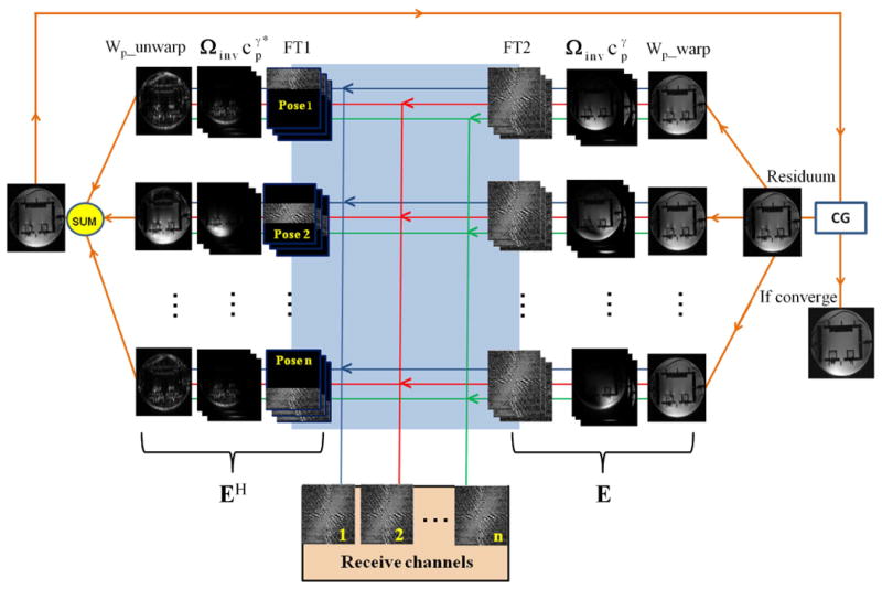
Flow diagram of the augmented SENSE reconstruction algorithm for combined correction of gradient distortions and sensitivity map variations.

The gridding was calculated using a Matlab toolbox provided by Fessler et al (22). The pose-dependent sensitivity maps were calculated as the division of individual-coil images (from constant pose data) by their sum-of-squares and further smoothed by performing 2D median filtering in a 3x3 window. The Cartesian coordinates (x_n y_n z_n) from tracking log files (each pose n) were transformed to spherical coordinates (r_n θ_n ϕ_n) and then directly applied to the SPH function to generate the gradient warping fields (23)

$$\mathrm{W}(\mathrm{r},\mathrm{\theta },\mathrm{\varphi })=\sum _{\ell }^{\mathrm{n}}\sum _{\mathrm{m}}^{\ell }{\mathrm{r}}^{\ell }[{\mathrm{a}}_{\ell }^{\mathrm{m}}cos(\mathrm{m}\mathrm{\varphi })+{\mathrm{b}}_{\ell }^{\mathrm{m}}sin(\mathrm{m}\mathrm{\varphi })]\times {\mathrm{P}}_{\ell }^{\mathrm{m}}(cos\mathrm{\theta })$$ [6]

where ${\mathrm{P}}_{\ell }^{\mathrm{m}}(cos\mathrm{\theta })$ is the associated Legendre polynomial. The variables ${\mathrm{a}}_{\ell }^{\mathrm{m}}$ and ${\mathrm{a}}_{\ell }^{\mathrm{m}}$ are the SPH coefficients of order ℓ and degree m which were provided by the scanner manufacturer. An unwarped image is obtained by interpolating the gray values in the warped image using a cubic interpolation (24) and vice versa as performed in the iterative loop (Fig. 1).

Reconstruction was performed using Matlab (version 12, The MathWorks Inc.), running on a Linux system. The residual errors of the reconstruction were depicted as a difference image (diff) between corrected images (at each iteration, im) and the reference (isocenter pose with gradient warp correction, ref) (i.e. diff = im - ref: pixel-wise subtraction of entire volume). Further quantitative analysis was done by considering the percentage error:

$$\%\text{error}={\text{RMS}}_{\text{diff}}/{\text{RMS}}_{\text{ref}}\times 100$$ [7]

where RMS_diff and RMS_ref are the root mean square of the difference and the reference images, respectively.

Simulations

The combined approach was tested in numerical simulations. The simulations were performed using the 3D Shepp-Logan phantom (25). The resolution was (1 mm)³ and the simulation volume (256 mm)³. Perfect prospective Mo-Co was assumed. Thus, the sensitivity maps and the gradient warp distortion moved relative to a stationary phantom. The eight sensitivity maps (c^γ) corresponding to each pose were approximated using 3D elliptic Gaussian functions:

$${\mathrm{c}}^{\mathrm{\gamma }}=exp(-([{(({\mathrm{x}}_{\mathrm{n}}-({\mathrm{x}}_0+\mathrm{\Delta }{\mathrm{x}}_{\mathrm{n}}))/\mathrm{a}]}^2+[{(({\mathrm{y}}_{\mathrm{n}}-({\mathrm{y}}_0+\mathrm{\Delta }{\mathrm{y}}_{\mathrm{n}}))/\mathrm{b}]}^2+[{(({\mathrm{z}}_{\mathrm{n}}-({\mathrm{z}}_0+\mathrm{\Delta }{\mathrm{z}}_{\mathrm{n}}))/\mathrm{a}]}^2))$$ [8]

The center points of the ellipses were defined by x₀ = 0, y₀ =FOV_y/2, and z₀ = 0 and shifted by Δx, Δy, and Δz. The values x_n, y_n, and z_n were obtained after rotating the xyz points of the initial pose (at isocenter) around the origin using R_xyzn, which is a product of rotation operators R_xn, R_yn, and R_zn of each pose n.

$${[{\mathrm{x}}_{\mathrm{n}}{\mathrm{y}}_{\mathrm{n}}{\mathrm{z}}_{\mathrm{n}}]}^{\mathrm{T}}={\mathbf{R}}_{\text{xyzn}}{[\text{xyz}]}^{\mathrm{T}}$$ [9]

The centers of the eight maps were equally separated. The ellipses were tilted such that the y-axis always pointed to the center of the volume. The gradient warp functions at the different poses were calculated using SPH as described in the previous section. The same 256 random numbers with standard deviation (SD) = 1 were used in every simulation. Thereby, any bias effect of different random motion generation on the motion artifacts was avoided. Three types of motion were generated as followed: Δx_n, Δy_n, Δz_n, and R_xn, R_yn, R_zn were set to be mild, moderate, and large motions by multiplying the normalized random numbers with 5, 10, and 30 mm or degrees, respectively. To assess the applicability of motion correction to more realistic situations than random motion, these numbers were rearranged into periodic motion with 4 oscillations as shown in Fig 2b.

Fig. 2.

a: Identically windowed images (selected slice) for three types of motion, the artifact increases with stronger motion (first two columns). The artifacts appear remarkably reduced by applying the proposed method (last four columns) (GW: the gradient warp correction). b: Six parameters of motion Δx, Δy, Δz, and R_x, R_y, R_z have the same pattern. These parameters were scale to be mild (±5 mm. and degrees), moderate (±10 mm. and degrees), or large (±30 mm. and degrees). c: The residual error as a function of iterations.

To construct motion-corrupted MR signals, first, the 3D phantom and 3D sensitivity profiles at each pose were warped. Individually corrupted images from coil γ were formed as the multiplication of the distorted phantom and distorted maps followed by FFT into k-space. Subsequently, data from coil γ and pose p (m_γ,p) were taken as the readout signal. The process was repeated for all phase encoding steps. The large linear problem was defined as Eq. 2. Note that we used the same motion information (moving coils and gradient warp functions) for both the generation of the motion-corrupted data and the motion correction process.

MR Experiments

Experiments were performed on a 7T Siemens scanner equipped with a 24-channel head coil. The imaging parameters were: 3D-FLASH, imaging volume 256x256x160 mm³, voxel size 1 mm³, TR 10 ms, TE 3.2 ms, FA 15°, BW 849 Hz/pixel, and TA 5.54 minutes. A moiré phase tracking (MPT) system was used in this study in order to maintain the pose of the image volume relative to the phantom in real time (26). The phantom was scanned at eight different constant poses to avoid any effects of internal motion in the object and potential inaccuracies, such as delays of the pose tracking. Synthetic 3D images corrupted by residual artifacts after prospective motion correction were created by mixing the k-space data from the eight constant poses. 32 phase encoding lines (along y-direction) of each constant pose were chosen to be a group of motion data (Fig. 3b).

Fig. 3.

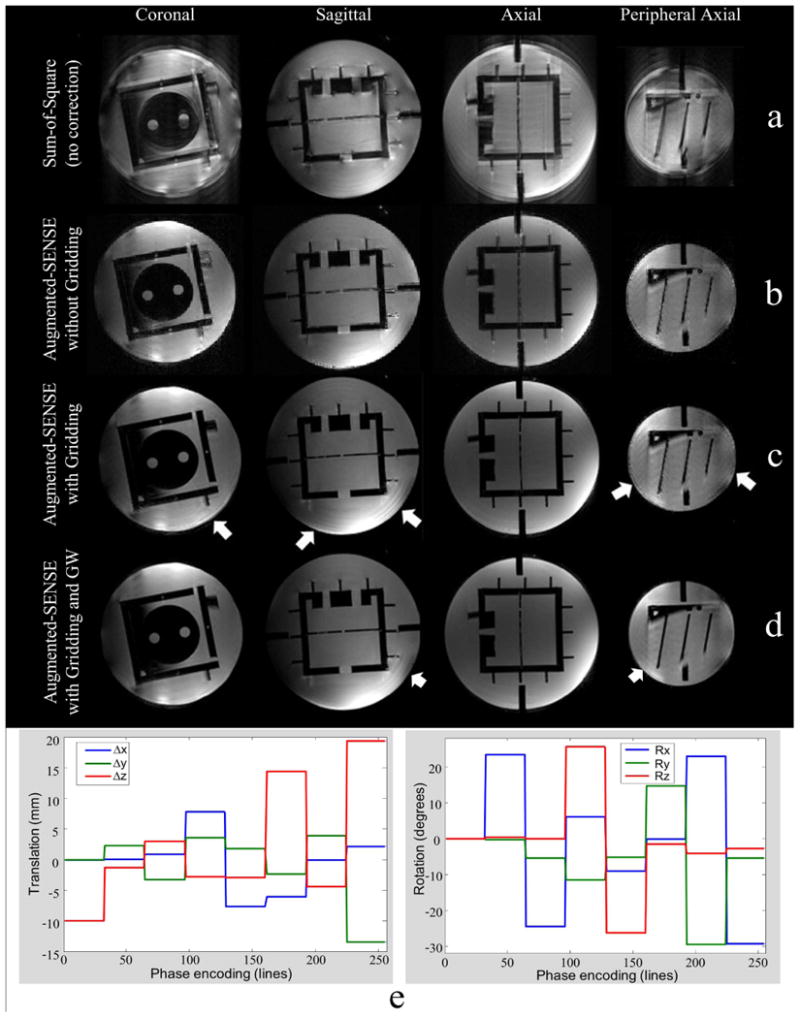
a: Mixed k-space data from different poses lead to strong artifact. b, c, and d are the 10^th iteration of augmented SENSE images. b: The intensity appear highly uniform after sensitivity maps correction. c: Blurring artifacts at the edge (white arrows) still remain after k-space and maps corrections. d: High image quality with very little remaining artifacts (white arrows) was achieved by the proposed method. e: The patterns of mixing experimental phantom k-space from eight different poses (32 lines per pose).

In order to avoid interaction between non-rigid distortion (the gradient nonlinearity and B0 inhomogeneity) and residual rigid motion due to imperfect cross-calibration or tracking noise of the camera system, retrospective registration (27) was applied to estimate the latter errors between each motion pose and the initial pose. Residual translation errors (Δx_i, Δy_i, Δz_i) were corrected applying a Fourier shift in k-space. Residual rotation errors (ΔR_xi, ΔR_yi, ΔR_zi) were considered during iterative CG by setting them to be Λ^res in order to grid k-space positions at each phase i [Eq. 3]. To reduce computation time and memory requirement a subset of eight receivers contributing the highest signal amplitude to the entire volume were selected for motion correction (28).

Results

Simulation Results

Fig. 2a shows that the gradient nonlinearity and the coil sensitivity misalignment can degrade the quality of perfect prospective Mo-Co images. The degradations increased with larger motion. The average percentage errors for mild, moderate, and large motions were 17.4%, 22.3%, and 33.2%, respectively. The proposed method reduced the artifacts notably for all types of motion - both shape and intensity of the corrupted images were recovered to almost the level of the reference after five iterations. The errors for mild, moderate, and large motions decreased from 13.1%, 16.9%, and 26.4% after the first iteration to 1.1%, 1.4%, and 2.6% after the fifth iteration.

Experimental Results

The artifacts caused by residual rigid motion, non-rigid distortion and sensitivity map variation are shown in Fig. 3a. The registration showed residual rigid body deviation of less than 0.5mm or 0.5 degrees. This is very small and thus k-space is almost homogeneously sampled. Ignoring retrospective k-space adjustment (here called gridding) in augmented SENSE, the images are acceptable as demonstrated in Fig. 3b. However, the images appear sharper when k-space was gridded. The central regions improve considerably while the residual blurring artifacts remain for both the edge of the center slice and more strongly at the periphery (Fig. 3c). This suggests that the artifacts cannot be compensated completely by this step alone. High image quality with very little remaining artifacts was achieved when the gradient warp correction was added (Fig. 3d). The error as a function of the number of iterations is shown in Fig. 4. The shape errors in particular at the edge of the phantom only disappear when the gradient warp correction was applied. The errors in augmented SENSE without and with the gradient warp correction reduce from 28.7% to 19.8% and from 25.7% to 17.3% after 10 iterations, respectively.

Fig. 4.

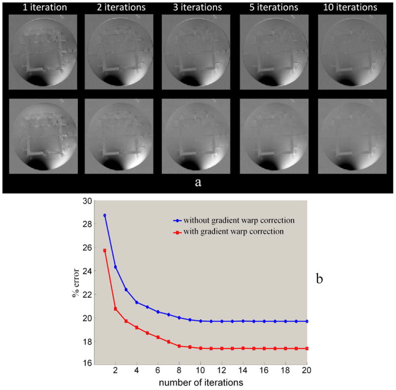
a: The visualization of residual errors when applying 1, 2, 3, 5, and 10 iterations (without and with gradient warp corrections shown in the 1^st and 2^nd rows, respectively). Note that the intensity variations (dark region) in the motion and the reference result the highly remaining percentage errors. b: The reduction of the artifacts with iteration number.

Discussion and Conclusions

Geometric distortions are a well-known problem in MRI, leading to pixel shifts with errors of up to several millimeters, thereby interfering with precise localization of anatomical structures. They can arise from a variety of sources such as the chemical shift, the magnetic susceptibility, eddy currents, B0 inhomogeneity, and gradient non-linearity (29). Aspects of geometric distortion due to gradient field non-linearity are the barrel distortion (2D and 3D), the potato chip effect (slice-selection, 2D), and the bow-tie effect (2D) (30). Correction of the potato chip distortion in multi-slice 2D acquisitions is not addressed in this work that focusses on 3D imaging. Both potato chip and bow-tie effects can be reduced considerably in 3D imaging where phase encoding is used in two directions with full volume excitation and weak or no slice selection gradient (31). The remaining barrel distortion in 3D acquisition can be corrected by applying a theoretically derived correction field as implemented in this study. Variations of the 2D slice selection distortion due to motion cause inconsistencies in single slice k-space data that will require a different approach for correction. The B0 inhomogeneity caused by magnetic properties of the object is frequently considered the main source of geometric distortions. When an object position or orientation changes, distortions due to local magnetic field inhomogeneity will change. It was shown (32, 33) that such motion-induced magnetic field changes caused non-rigid geometric distortion particularly in echo-planar imaging (EPI) which is most sensitive to field inhomogeneity due to the low effective phase-encoding bandwidth. In this study, the effects and correction of gradient non-linearity in conventional 3D imaging were considered, where distortions are lower than in EPI yet still considerable as shown in the motion corrected date without gradient correction. The very small susceptibility phantom and high sampling bandwidth were used. The changes of the B0 field were measured for the different poses and the displacements were below 0.3 mm. This is approx. 8 times smaller than displacements caused by gradient non-linearity (Fig. 5). Therefore, gradient imperfections here are the dominant cause of residual artifacts after rigid body motion correction. However, small remaining artifacts (white arrow in Fig. 3d) still appeared after correcting gradient non-linearity. These may be caused by residual B0-field inhomogeneity variations. It was observed in 3T MRI (34) that maximum distortions near air-tissue interfaces was less than 4 mm and fell to less than 1 mm at a distance of 8 mm from the interface. This may become more critical at higher field strength and B0-inhomogeneity may become more relevant. The relative contribution of gradient- and susceptibility-induced distortions will likely determine the relevance of the proposed correction.

Fig. 5.

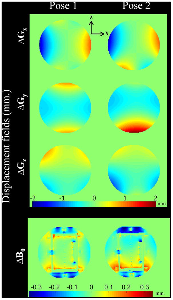
The change of displacements (in millimeter) of the three gradients (ΔG_x, ΔG_y, ΔG_z) and the main magnetic field (ΔB₀) corresponding to the chosen coronal slice at isocenter (Pose1) and 25 mm off-isocenter along the -Z direction (Pose2). Note that the B0 induced shift is much smaller than the gradient distortion for the FLASH sequence used.

The application of the proposed method to experimental data demonstrated a clear improvement in image quality especially in off-center slices. The reconstruction required slightly more iterations than predicted from the simulation. This may be because the coil sensitivity distribution around the sample is not uniform as in the simulation. This also causes the intensity variations between the corrected and the reference images. Consequently, the percentage errors of the proposed reconstruction remain higher than in the simulation (Fig. 4). Note that the diameter of the Shepp-Logan phantom was approximately 220 mm and thus larger than the experimental phantom (∼150 mm). The gradient non-linearity artifact is thus more prominent in the simulation than in the experimental data especially in peripheral regions. We demonstrate that this effect is more pronounced in off-center areas, i.e. for large objects and large object motion. As studied by Wang et al (35), the gradient field non-linearity in five different gradient sets varied strongly. Within a volume of (240 mm)³, the geometric errors were between 10 and 25 mm in MRI systems equipped with fast gradient systems while MRI systems equipped with conventional gradient systems showed only 2 to 4 mm errors. Other authors have reported maximum distortions over similar (but not identical) imaging volumes of: 9 mm at 1.5T (15), 7 mm at 3T (16). In this study, the maximum gradient-related displacements based on the manufacturer's SPH coefficients in measurement volumes of 200, 240 or (300 mm)³ are 6.7, 14.5 or 43.8 mm, respectively. Therefore, the relevance of the gradient non-linearity correction in prospective motion correction will vary depending on the design of the gradient system.

In practice, several challenges require further investigation. First and common with the original augmented SENSE method, the explicit determination of 3D sensitivity maps for each motion pose is impractical and time consuming. Banerjee S. et al (36) showed that the maps for different poses can be generated by re-gridding the initial dataset. However, this method is limited if the object moves outside the area covered by the initial sensitivity maps. Second, the residual tracking errors were estimated by 3D rigid body registration in this study, which may be impractical for partial k-space data. This procedure is not required for highly accurate tracking. However, as demonstrated by Maclaren et al (37), several factors can compromise the accuracy of tracking systems e.g., the effect of tracking noise and the delay in the calculation and feedback of pose information. These factors are unlikely sources in the current study as the object was stationary during scanning. Furthermore, it may also be that the calibration of the tracking system itself is influenced by gradient distortion errors. The cross-calibration procedure, which is based on image registration can be compromised by gradient non-linearity in particular for large scale motion as required in this procedure (9). Gradient non-linearity should therefore be considered in the cross-calibration procedure. The determination of the residual rigid motion error may itself be impacted by the distortion of the images that are registered. This residual error was much smaller than the object motion and should be further reduced or even negligible once the distortion is considered during the calibration.

In conclusion, this study demonstrates that geometric distortions due to gradient non-linearity induce residual artifacts even in perfectly prospectively motion-corrected data, in particular in off-center regions. These artifacts can be mitigated by adding a 3D gradient warp correction of partial k-space data into the augmented SENSE reconstruction. The combined correction of gradient non-linearity and sensitivity map variation leads to a pronounced reduction of residual motion artifacts in prospectively motion-corrected data.

References

- 1.Ehman RL, Felmlee JP. Adaptive technique for high-definition MR imaging of moving structures. Radiology. 1989;173(1):255–263. doi: 10.1148/radiology.173.1.2781017. [DOI] [PubMed] [Google Scholar]
- 2.Pipe JG. Motion correction with PROPELLER MRI: application to head motion and free-breathing cardiac imaging. Magn Reson Med. 1999;42(5):963–969. doi: 10.1002/(sici)1522-2594(199911)42:5<963::aid-mrm17>3.0.co;2-l. [DOI] [PubMed] [Google Scholar]
- 3.Derbyshire JA, Wright GA, Henkelman RM, et al. Dynamic scan-plane tracking using MR position monitoring. J Magn Reson Imaging. 1998;8(4):924–932. doi: 10.1002/jmri.1880080423. [DOI] [PubMed] [Google Scholar]
- 4.Bydder M, Larkman DJ, Hajnal JV. Detection and elimination of motion artifacts by regeneration of k-space. Magn Reson Med. 2002;47(4):677–686. doi: 10.1002/mrm.10093. [DOI] [PubMed] [Google Scholar]
- 5.Atkinson D, Hill DL, Stoyle PN, Summers PE, Clare S, Bowtell R, Keevil SF. Automatic compensation of motion artifacts in MRI. Magn Reson Med. 1999;41(1):163–170. doi: 10.1002/(sici)1522-2594(199901)41:1<163::aid-mrm23>3.0.co;2-9. [DOI] [PubMed] [Google Scholar]
- 6.Batchelor PG, Atkinson D, Irarrazaval P, Hill DL, Hajnal J, Larkman D. Matrix description of general motion correction applied to multishot images. Magn Reson Med. 2005;54(5):1273–1280. doi: 10.1002/mrm.20656. [DOI] [PubMed] [Google Scholar]
- 7.Thesen S, Heid O, Mueller E, Schad LR. Prospective acquisition correction for head motion with image-based tracking for real-time fMRI. Magn Reson Med. 2000;44(3):457–465. doi: 10.1002/1522-2594(200009)44:3<457::aid-mrm17>3.0.co;2-r. [DOI] [PubMed] [Google Scholar]
- 8.Ward HA, Riederer SJ, Grimm RC, Ehman RL, Felmlee JP, Jack CR., Jr Prospective multiaxial motion correction for fMRI. Magn Reson Med. 2000;43(3):459–469. doi: 10.1002/(sici)1522-2594(200003)43:3<459::aid-mrm19>3.0.co;2-1. [DOI] [PubMed] [Google Scholar]
- 9.Zaitsev M, Dold C, Sakas G, Hennig J, Speck O. Magnetic resonance imaging of freely moving objects: prospective real-time motion correction using an external optical motion tracking system. NeuroImage. 2006;31(3):1038–1050. doi: 10.1016/j.neuroimage.2006.01.039. [DOI] [PubMed] [Google Scholar]
- 10.Maclaren J, Herbst M, Speck O, Zaitsev M. Prospective motion correction in brain imaging: a review. Magn Reson Med. 2013;69(3):621–636. doi: 10.1002/mrm.24314. [DOI] [PubMed] [Google Scholar]
- 11.Atkinson D, Larkman DJ, Batchelor PG, Hill DL, Hajnal JV. Coil-based artifact reduction. Magn Reson Med. 2004;52(4):825–830. doi: 10.1002/mrm.20226. [DOI] [PubMed] [Google Scholar]
- 12.Liu C, Moseley ME, Bammer R. Simultaneous phase correction and SENSE reconstruction for navigated multi-shot DWI with non-cartesian k-space sampling. Magn Reson Med. 2005;54(6):1412–1422. doi: 10.1002/mrm.20706. [DOI] [PubMed] [Google Scholar]
- 13.Bammer R, Aksoy M, Liu C. Augmented generalized SENSE reconstruction to correct for rigid body motion. Magn Reson Med. 2007;57(1):90–102. doi: 10.1002/mrm.21106. [DOI] [PMC free article] [PubMed] [Google Scholar]
- 14.Wang D, Strugnell W, Cowin G, Doddrell DM, Slaughter R. Geometric Distortion in Clinical MRI Systems Part II: Correction Using a 3D Phantom. J Magn Reson Imaging. 2004;22:1223–1232. doi: 10.1016/j.mri.2004.08.014. [DOI] [PubMed] [Google Scholar]
- 15.Doran SJ, Charles-Edwards L, Reinsberg SA, Leach MO. A complete distortion correction for MR images: I. Gradient warp correction. Phys Med Biol. 2005;50:1345–1361. doi: 10.1088/0031-9155/50/7/001. [DOI] [PubMed] [Google Scholar]
- 16.Baldwin LN, Wachowicz K, Thomas SD, Rivest R, Gino Fallone B. Characterization, prediction and correction of geometric distortion in 3 T MR images. Medical Physics. 2007;34(2):388–399. doi: 10.1118/1.2402331. [DOI] [PubMed] [Google Scholar]
- 17.Langlois S, Desvignes M, Constans JM, Revenu M. MRI geometric distortion: a simple approach to correcting the effects of non-linear gradient fields. J Magn Reson Imaging. 1999;9(6):821–831. doi: 10.1002/(sici)1522-2586(199906)9:6<821::aid-jmri9>3.0.co;2-2. [DOI] [PubMed] [Google Scholar]
- 18.Polzin JA, Kruger DG, Gurr DH, Brittain JH, Riederer SJ. Correction for gradient nonlinearity in continuously moving table MR imaging. Magn Reson Med. 2004;52(1):181–187. doi: 10.1002/mrm.20117. [DOI] [PubMed] [Google Scholar]
- 19.Hu HH, Madhuranthakam AJ, Kruger DG, Glockner JF, Riederer SJ. Continuously moving table MRI with SENSE: application in peripheral contrast enhanced MR angiography. Magn Reson Med. 2005;54(4):1025–1031. doi: 10.1002/mrm.20639. [DOI] [PMC free article] [PubMed] [Google Scholar]
- 20.Luengviriya C. Necessity of sensitivity profile correction in retrospective motion correction. Proceedings of the 18th Annual Meeting of ISMRM; Stockholm, Sweden. 2010. Number 3064. [Google Scholar]
- 21.Pruessmann KP, Weiger M, Bornert P, Boesiger P. Advances in sensitivity encoding with arbitrary k-space trajectories. Magn Reson Med. 2001;46(4):638–651. doi: 10.1002/mrm.1241. [DOI] [PubMed] [Google Scholar]
- 22.Jeff Fessler. Image reconstruction toolbox. [Accessed October 15, 2012]; The University of Michigan Web site. http://web.eecs.umich.edu/∼fessler/irt/fessler.tgz.
- 23.Janke A, Zhao H, Cowin GJ, Galloway GJ, Doddrell DM. Use of spherical harmonic deconvolution methods to compensate for nonlinear gradient effects on MRI images. Magn Reson Med. 2004;52(1):115–122. doi: 10.1002/mrm.20122. [DOI] [PubMed] [Google Scholar]
- 24.Robert G. Keys. Cubic Convolution Interpolation for Digital Image Processing. IEEE Trans on Acoustics, Speech, and Signal Processing. 1981;29(6):1153–1160. [Google Scholar]
- 25.Koay CG, Sarlls JE, Ozarslan E. Three Dimensional Analytical Magnetic Resonance Imaging Phantom in the Fourier Domain. Magn Reson Med. 2003;58:430–436. doi: 10.1002/mrm.21292. [DOI] [PubMed] [Google Scholar]
- 26.Maclaren J, Armstrong BSR, Barrows RT, et al. Measurement and Correction of Microscopic Head Motion during Magnetic Resonance Imaging of the Brain. PLoS ONE. 2012 doi: 10.1371/journal.pone.0048088. http://dx.doi.org/10.1371/annotation/a29733ae-6317-42ee-92c0-a49542e1b7c8. [DOI] [PMC free article] [PubMed]
- 27.Kroon Dirk-Jan. multimodality non-rigid demon algorithm image registration. [Accessed December 1, 2012]; Mathworks Web site. http://www.mathworks.com/matlabcentral/fileexchange Published September 16, 2008. Updated Junuary 03, 2010.
- 28.Luengviriya C. ISMRM Workshop on Current Concepts of Motion Correction for MRI & MRM. Kitzbuhel; Tyrol, Austria: 2010. Necessity of sensitivity profile correction in retrospective motion correction at 7T MRI. [Google Scholar]
- 29.Archip N, Clatz O, Whalen S, Dimaio SP, Black PM, Jolesz FA, Golby A, Warfield SK. Compensation of geometrical distortion effects on intraoperative magnetic resonance imaging for enhanced visualization in image-guided neurosurgery. Neurosurgery. 2008;62:209–216. doi: 10.1227/01.neu.0000317395.08466.e6. [DOI] [PubMed] [Google Scholar]
- 30.Sumanaweera T, Adler JR, Napel S, Glover GH. Characterization of spatial distortion in magnetic resonance imaging and its implications for stereotaxic surgery. Neurosurgery. 1994;35(4):696–704. doi: 10.1227/00006123-199410000-00016. [DOI] [PubMed] [Google Scholar]
- 31.Walton L, Hampshire A, Forster DMC, Kemeny AA. Stereotactic localization with magnetic resonance imaging: a phantom study to compare the accuracy obtained using two-dimensional and three-dimensional data acquisitions. Neurosurg. 1997;41(1):131–139. doi: 10.1097/00006123-199707000-00027. [DOI] [PubMed] [Google Scholar]
- 32.van der Kouwe Andr JW, Benner Thomas, Anders M Dale. Real-time rigid body motion correction and shimming using cloverleaf navigators. Magn Reson Med. 2006;56(5):1019–1032. doi: 10.1002/mrm.21038. [DOI] [PubMed] [Google Scholar]
- 33.Ooi MB, Muraskin J, Zou X, et al. Combined prospective and retrospective correction to reduce motion-induced image misalignment and geometric distortions in EPI. Magn Reson Med. 2013;69(3):803–811. doi: 10.1002/mrm.24285. [DOI] [PMC free article] [PubMed] [Google Scholar]
- 34.Wang H, Balter J, Cao Y. Patient-induced susceptibility effect on geometric distortion of clinical brain MRI for radiation treatment planning on a 3T scanner. Phys Med Biol. 2013;58(3):465–77. doi: 10.1088/0031-9155/58/3/465. [DOI] [PubMed] [Google Scholar]
- 35.Wang D, Strugnell W, Cowin G, Doddrell DM, Slaughter R. Geometric Distortion in Clinical MRI Systems Part I: Evaluation Using a 3D Phantom. Magn Reson Imaging. 2004;22(9):1211–21. doi: 10.1016/j.mri.2004.08.012. [DOI] [PubMed] [Google Scholar]
- 36.Banerjee S, Beatty PJ, Zhang JZ, Shankaranarayanan A. Parallel and partial Fourier imaging with prospective motion correction. Magn Reson Med. 2013;69(2):421–433. doi: 10.1002/mrm.24269. [DOI] [PubMed] [Google Scholar]
- 37.Maclaren J, Lee KJ, Luengviriya C, Speck O, Zaitsev M. Combined prospective and retrospective motion correction to relax navigator requirements. Magn Reson Med. 2011;65(6):1724–1732. doi: 10.1002/mrm.22754. [DOI] [PubMed] [Google Scholar]