

Abstract
Purpose
To propose and evaluate a novel non-rigid image registration approach for improved myocardial T1 mapping.
Methods
Myocardial motion is estimated as global affine motion refined by a novel local non-rigid motion estimation algorithm. A variational framework is proposed, which simultaneously estimates motion field and intensity variations, and uses an additional regularization term to constrain the deformation field using automatic feature tracking. The method was evaluated in 29 patients by measuring the DICE similarity coefficient (DSC) and the myocardial boundary error (MBE) in short axis and four chamber data. Each image series was visually assessed as “no motion” or “with motion”. Overall T1 map quality and motion artifacts were assessed in the 85 T1 maps acquired in short axis view using a 4-point scale (1-non diagnostic/severe motion artifact, 4-excellent/no motion artifact).
Results
Increased DSC (0.78±0.14 to 0.87±0.03, p<0.001), reduced MBE (1.29±0.72mm to 0.84±0.20mm, p<0.001), improved overall T1 map quality (2.86±1.04 to 3.49±0.77, p<0.001), and reduced T1 map motion artifacts (2.51±0.84 to 3.61±0.64, p<0.001) were obtained after motion correction of “with motion” data (~56% of data).
Conclusion
The proposed non-rigid registration approach reduces the respiratory-induced motion that occurs during breath-hold T1 mapping, and significantly improves T1 map quality.
Keywords: Myocardial Tissue Characterization, T1 Mapping, Motion correction, Motion estimation, Image registration
INTRODUCTION
Expansion of the myocardial extracellular space occurs in a variety of cardiovascular disease (1–3). Late gadolinium enhancement (LGE) is the gold standard technique for imaging of localized myocardial extracellular space expansion as typically encountered in the presence of focal fibrosis and scar (4,5). LGE imaging relies on the presence of intensity variation between fibrosis/scar and healthy myocardium. This technique may be limited for the assessment of more diffuse disease (6). Myocardial T1 mapping is an emerging technique for the assessment of diffuse interstitial fibrosis (7). Pre-contrast and post-contrast T1 mapping can be acquired to quantify the extracellular volume (ECV) (8), which shows promise for the assessment of diffuse interstitial fibrosis (9,10).
Quantitative myocardial T1 mapping is commonly performed using a breath-hold ECG-triggered acquisition over ~9–13 heart beats (11–14). One T1-weighted image is generally acquired per heart beat during the mid-diastolic cardiac period which corresponds to the more quiescent phase of the cardiac cycle. Pixel-wise T1 estimation is then performed by fitting T1-weighted images to the T1 recovery curve. To enable reliable pixel-wise T1 fitting, the pixel across different T1-weighted images should be aligned. However, despite breath-hold instructions, motion is observed in 40–50% of patients due to diaphragmatic drift and their limited breath-holding capability (15,16), which leads to significant imaging artifacts in T1 maps. Respiratory motion correction techniques are thus required to improve the quality of T1 maps.
Image-based motion correction algorithms can be used to reduce in-plane motion among T1-weighted images (15,16). Although a variety of motion estimation algorithms have been proposed for medical image registration (17) and specifically to cardiac image registration (18), few studies have addressed the motion problem in myocardial T1 mapping. Motion correction of T1-weighted image series is challenging due to the high contrast variation among T1-weighted images. Intensity-based approaches have been shown to fail due to the presence of high contrast variation and transient tissue nulling at certain inversion times (16).
A recent approach (16) used synthetic T1-weighted images to simplify the registration problem in Modified Look-Locker Inversion Recovery (MOLLI) data (12). Synthetic T1-weighted images were created from T1 estimates to simulate motion corrected MOLLI data. The polarity of each acquired T1-weighted image is then restored using a multi-fitting approach (19) and each pair of T1-weighted images (acquired and simulated) is then registered together. This process is iterated to reduce the impact of initial T1 estimate errors. A proposed extension of this method uses an alternative approach for signal polarity restoration based on phase sensitive inversion recovery (PSIR) reconstruction (15). The PSIR reconstruction used the phase information of the T1-weighted image acquired with the longest recovery period of each Look-Locker experiment (20) to restore the polarity. This method was found more efficient than the multi-fitting approach for the restoration of the signal polarity (15). However, the efficiency of such algorithms could be suboptimal in the presence of large motion where large bias and artifacts are generally observed in the initial T1 estimates. In addition the PSIR reconstruction may also fail to accurately restore the signal polarity in the presence of large motion within each Look Locker experiment (15).
In this study, we propose and evaluate a novel motion correction algorithm for T1 mapping which directly relies on the acquired T1-weighted images and does not require the restoration of the signal polarity.
METHODS
We propose a novel image-based approach for Adaptive Registration of varying Contrast-weighted images for improved TIssue Characterization (ARCTIC) and evaluate its performance for myocardial T1 mapping applications. Figure 1 shows the general scheme of the algorithm. Each T1-weighted image is individually registered to a common reference T1-weighted image using a two-step approach. In the proposed approach, a region of interest (ROI) is first manually drawn around the left ventricle (LV) of the reference image (LV-ROI). All subsequent steps are performed automatically. The global affine motion of the LV is first estimated using a region-matching algorithm. The motion estimates are then refined using a novel local non-rigid motion estimation approach based on an extended optical flow formulation.
Figure 1.
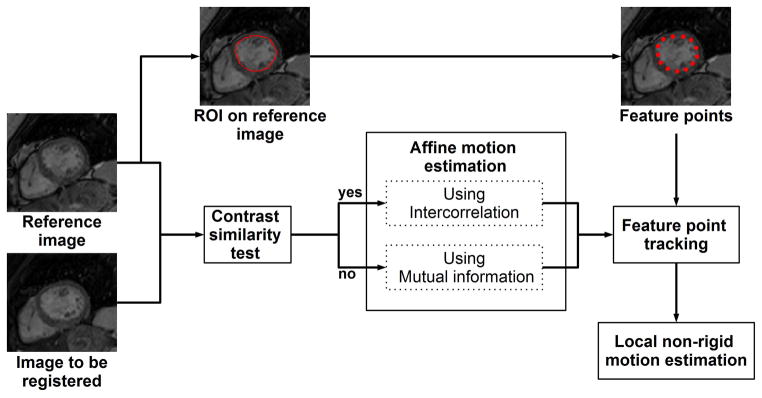
General scheme of the ARCTIC approach. A dense motion field is estimated between each T1-weighted image and a reference image which is chosen as the fourth image of the image series. A region-of-interest (ROI) is initially drawn manually on the reference image to delineate the endocardial border of the myocardium. Endocardial points (feature points) are then extracted by regular sampling of the ROI edges. Each T1-weighted image is then registered to the reference image using the following steps. The contrast similarity between the reference image and the image to register is first assessed using an heuristic approach. Affine motion parameters are then estimated over the ROI by maximization of the inter-correlation coefficient (positive contrast similarity test) or the mutual information (negative contrast similarity test). Subsequently, the displacement of each feature point is estimated using the affine motion parameters as pre-conditioning. Local non-rigid motion estimation is finally performed to refine affine motion estimates and uses an extended formulation of the optical flow problem which simultaneously estimates motion field and intensity variation and integrates the displacement of feature points as an additional regularization term.
Step I: Global Motion Estimation
The coarse LV motion is first estimated using a region-matching approach (21) where a unique set of affine motion parameters is estimated to represent the LV motion. A sign gradient-descent with fixed steps (22,23) is employed to obtain the affine motion parameters, which maximize a similarity criterion between the reference image and the registered image within the LV-ROI. The similarity criterion was defined for each image to register as the inter-correlation or the mutual information. This choice was based on the intensity/contrast similarity (C) between the reference image and the image to register. C was computed using the following heuristic:
| [1] |
where Iref is the reference image, I2reg is the image to register, and M is the reference binary mask set to 1 inside the LV-ROI and 0 elsewhere. For T1-weighted images with similar intensity/contrast as the reference image (empirically defined as C ≤ 0.8), the similarity criterion is defined as the inter-correlation coefficient (EInt):
| [2] |
where S is the number of pixels set to 1 in M, and ( ; σIref), ( , σI2reg) are the (averaged; standard deviation) of Iref and I2reg over all pixels satisfying M(x,y) = 1, respectively. For T1-weighted images depicting different intensity/contrast than the reference image (C > 0.8), the mutual information (EMut) is used as similarity criterion as follows:
| [3] |
where ρ is the joint probability distribution function of the image intensity of Iref and I2reg and (ρIref, ρI2reg) are the marginal probability distribution functions of the image intensity of Iref and I2reg, respectively. N (empirically set to 100) is the bin number of the histograms used for the calculation of ρIref, ρI2reg and ρ. Note that, when using the mutual information, the LV-ROI is dilated using a local maximum operator (empirically defined as a disk structuring element with ray of 20 pixels) to improve the metric robustness. Finally, the estimated set of affine motion parameters is converted to a dense motion field (one 2D displacement vector per pixel) and used as initialization of a local non-rigid motion estimation algorithm.
Step II: Local Non-Rigid Motion Estimation
Optical flow (OF) algorithms (24–26) estimate dense motion fields by assuming intensity conservation during object displacements over time. Let be I(x,y,t) the image intensity of the reference image at pixel coordinates (x,y) at time t. The intensity conservation hypothesis leads to model the displacement (dx,dy) during time dt as:
| [4] |
The first-order Taylor series expansion about I(x,y,t) reads as:
| [5] |
with (Ix, Iy, It) = (∂I/∂x, ∂I/∂yx, ∂I/∂t) and where ε represents the high order terms. Ignoring ε (which hold for small displacements) and combining equations [4] and [5] lead to the optical flow equation:
| [6] |
where (u, v) = (dx/dt, dy/dt) is the 2D velocity field or optical flow.
However, the intensity conservation hypothesis does not hold for T1-mapping application where the images depict dramatic contrast/intensity variations due to different T1-weighting. Therefore, we propose to integrate the intensity variation between T1-weighted images as part of the motion model as follows:
| [7] |
where c(x,y,t) is the pixel-wise intensity variation. Using equations [5] and [7], a modified formulation of the optical flow equation can be written as:
| [8] |
Equation [8] has 3 unknowns (2D motion field (u,v), and intensity variation (c)) which need to be estimated. Therefore, to solve this ill-posed problem, additional constraints are needed. Horn and Schunck proposed to constrain the spatial smoothness of the motion field in the initial formulation of the optical flow (equation [6]) (24). This framework was then extended by Cornelius and Kanade (27) to solve equation [8] where the spatial smoothness of both motion field and intensity variation was constrained. The optical flow is then estimated by minimization of the following functional:
| [9] |
where α is a weighting parameter designed to control the spatial smoothness of the motion field β is a weighting parameter which controls the spatial smoothness of the intensity variation c, and ∇u = (du/dx, du/dy), ∇v = (dv/dx, dv/dy), ∇c = (dc/dx, dc/dy).
To improve the robustness of the algorithm in the presence of transient structures induced by out-of-plane motion and specific tissue nulling at certain inversion time, we propose to add an additional regularization term which constrains the motion estimates using pre-estimated displacements of specific feature points (22). Feature points are obtained by regular sampling of the LV-ROI contour. The displacement of each feature point is automatically estimated using a region-matching approach restrained to a small ROI centered on each of these points. A simple 2D translational model is estimated for each feature point to maintain the robustness of the estimation. The similarity metric used for region matching is based on the edge orientation coincidence function Eedge (28) and is defined as:
| [10] |
where M is a binary mask set to 1 inside the feature point ROI and 0 elsewhere, S is the edge strength defined as , Δθ is the edge orientation variation defined as Δθ = tan−1(GyIref/GxIref) − tan−1 (GyI2reg/GxI2reg). To speed up the convergence of the feature point tracking step, the 2D translational displacement of each feature point is estimated using a sign gradient-descent with fixed steps (22,23) with the global motion estimate as initialization. To remove occasional non-physiological motion estimates, an outlier rejection is added. The motion estimates of the feature points are assumed to follow a bivariate Gaussian distribution. A feature point is automatically discarded if at least one of its displacement components does not lie within three standard deviations of the averaged feature point displacements (marginal three-sigma rule). The displacement of these feature points is then integrated into a novel variation formulation of the optical flow problem as follows:
| [11] |
where (ui, vi) are the pre-estimated 2D displacements of each feature point, N is the number of feature points, λ is a weighting parameter, and F(di) is a distance function defined as:
| [12] |
where d represents the Euclidean distance between the pixel coordinates (x,y) and the ith feature point, and R controls the spatial influence of each constraint point. The optical flow is finally obtained by minimization of the functional EARCTIC(u,v,c) using the calculus of variation and the Gauss-Seidel approach as described in Appendix A.
Experimental Evaluation
Twenty-nine patients referred for clinical CMR (58±15 y, 19 male) were recruited. Informed consent was obtained from all participants and the imaging protocol was approved by our institutional review board. All patients were scanned using a 1.5T Philips Achieva (Philips Healthcare, Best, The Netherlands) scanner with a 32-channel cardiac phased array receiver coil. Each patient received an injection of 0.1 mmol/kg of gadobenate dimeglumine (MultiHance; Bracco Diagnostic Inc., Princeton, NJ). T1 mapping was performed using the MOLLI sequence (12) before and after contrast administration. The 5-(3)-3 MOLLI scheme was used for pre-contrast T1 mapping while the 4-(1)-3-(1)-2 MOLLI scheme was used for post contrast T1 mapping (29). Both sequences used a balanced-SSFP readout (TR/TE=3.1/1.5ms, FOV=360×337 mm2, acquisition matrix=188×135, voxel size=1.9×2.5 mm2, slice thickness=8 mm, number of phase-encoding lines=70, linear ordering, 10 linear ramp-up pulses, SENSE factor=2, flip angle=35/70°, bandwidth=1085Hz/pixel). T1 scans have been acquired in the short axis views using either 1 or 3 slices for the first 20 patients. A single slice has been acquired in the four chamber orientation for the last nine patients. Three T1 scans were acquired for each patient: one before contrast injection, and two post-contrast scans at 15±5 min and 31±6 min after contrast injection, respectively. Note that post-contrast T1 mapping could not be performed in all patients.
Implementation
We implemented ARCTIC using both central processing unit (CPU) and graphic processing unit (GPU) to enable efficient computation. C++ was used for CPU implementation and compute unified device architecture (CUDA) was used for GPU implementation. In this CPU/GPU implementation, the iterative scheme of the optical flow (equation 17), which is the most computationally intensive step of the algorithm, was offloaded to the GPU. The rest of the algorithm was performed on the CPU. The CPU/GPU implementation was compared to a CPU only implementation entirely developed in C++.
Two approaches for automatic selection of the reference image were evaluated. In short axis data, the reference image was chosen as the 4th image since it has a long inversion time with the employed pre-contrast (second longest TI) and post-contrast (longest TI) MOLLI imaging schemes. In four chamber data, the reference image was selected as the image with the longest inversion time (5th and 4th image in pre-contrast and post contrast image series, respectively). In both cases, the reference image is located at the middle of each acquisition, which is favorable to minimize the motion amplitude to be estimated in the presence of drifting motion. A multi-resolution approach (30) was used for the non-rigid motion estimation step where the optical flow is initially estimated from first sub-resolution images and then refined using the full resolution images. For each resolution level, the iterative scheme (equation [17]) used 100 iterations and was repeated five times.
T1 map reconstruction
T1 maps were reconstructed offline before and after motion correction. The restoration of the signal polarity among initial and motion corrected T1-weighted images was performed using a multi-fitting approach (19). Several T1 fits were performed by inverting the signal magnitude of none of the points, the point with the shortest inversion time, the two points with the shortest inversion times, and so on. The correct polarity restoration is selected from the dataset leading to the smallest residual fitting error. Pixel-wise T1 fitting was performed in two steps. Apparent T1 values were first estimated using a three point model (31) as follows:
| [13] |
where S(x,y,tn) is the signal of the nth T1-weighted image acquired at time tn after the last inversion pulse. A, B, and are the parameters estimated from the fit. A Marquard-Levenberg optimizer was employed to converge to the solution using the code provided in (32). To speed up the convergence of the estimation and avoid local minimum, B was initialized to 1 and (A; ) were initialized using a 2-parameter grid search. T1 values were then computed from apparent T1 estimates as:
| [14] |
Data analysis
The relative amount of motion estimated from the global affine motion estimation step and the local non-rigid motion estimation step is reported. The amount of motion was measured as the average L2 norm (over the myocardium) of the relative estimated motion field.
To quantify the accuracy of the ARCTIC approach, endocardial and epicardial contours were manually drawn in all T1-weighted images of all uncorrected MOLLI series. Both contours were converted into binary mask set to 1 inside the contour and 0 outside. A binary representation of the myocardium was obtained by computing the difference between the epicardial binary mask and the endocardial binary mask. The myocardial binary mask of each T1-weighted image was then registered to the binary mask of the reference image using the estimated motion field of each T1-weighted image. The DICE similarity coefficient (DSC) (33) was then calculated between the myocardial binary mask of the reference image and the registered myocardial binary mask of each T1-weighted image as follows:
| [15] |
where Mref and Mreg are myocardial binary masks of the reference image and the registered image, respectively. An ideal registration leads to a perfect overlap between both masks and would provide a DSC of 1. A DSC of 0 corresponds to the absence of overlap.
The myocardial boundary error (MBE) is also calculated to provide a local alignment measure. The myocardial boundary was first calculated for each T1-weighted image using the binary representation of the myocardium obtained from the endocardial and epicardial contours. MBE was measured as the average distance between the myocardial boundary of a T1-weighted image and the myocardial boundary of the reference image.
DSCs and MBEs are reported for uncorrected data (using the original encodardial/epicardial contours) and for motion corrected data (using the registered endocardial/epicardial contours). The averaged DSC (and MBE), over all 8(pre-contrast)/9(post-contrast) T1-weighted images, is reported for each MOLLI acquisition. In order to quantify the overall registration performance for each T1-weighted image of a MOLLI acquisition, the averaged DSC (and MBE) over all MOLLI acquisitions is reported for each of the 8/9 T1-weighted images. The statistical significant difference between DSCs (and MBEs) obtained with and without motion correction was evaluated using paired t-tests. Statistical significance was considered at p < 0.05.
T1-map reconstructed from motion corrupted T1-weighted images can depict severe artifacts as shown in Figure 2. Therefore, a subjective qualitative analysis was then conducted by an experienced cardiologist to assess the value of uncorrected and motion corrected T1 maps. The presence or absence of motion was first assessed for each image series by visual inspection of all T1-weighted images. Each image series was subsequently classified as “with motion” or “no motion”. Original (uncorrected) and motion corrected T1 maps (85×2=170 T1 maps) were also created for each image series acquired in the short axis view and assessed in term of overall T1 map quality and level of motion artifacts using a 4-point scale (1-non diagnostic/severe motion artifact, 2-fair/large motion artifacts, 3-good/small motion artifacts, 4-excellent/no motion artifact) (34). Figure 3 shows example of T1 maps with associated subjective scores. The reader was blinded to the study design and whether the T1 maps were motion corrected or not. Wilcoxon signed rank test was used to test the null hypothesis that the difference of overall T1 map quality scores/motion artifact scores between uncorrected and motion corrected T1 maps was zero. Mann-Whitney U-test was used to test the null hypothesis that the difference of overall T1 map quality scores/motion artifact scores between “no motion” data and “with motion” data was zero. Statistical significance was considered at p < 0.05.
Figure 2.
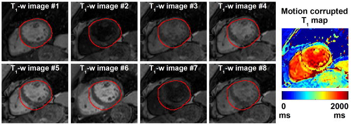
Example of motion corrupted T1-weighted image series. To facilitate visual motion assessment, the epicardial contour of the myocardium was drawn on the first T1-weighted image and is overlaid in all other images (red contours). Large drifting motion can be observed between the T1-weighted images which results in large artifacts, and a non-diagnostic T1 map.
Figure 3.

Illustration of the four-point scale used for assessment of overall T1 map quality and motion artifacts. Pre-contrast T1 maps with a score of, a) 1-non diagnostic/severe motion artifact, b) 2-fair/large motion artifacts, c) 3-good/small motion artifacts, and d) 4-excellent/no motion artifact (d) are shown.
RESULTS
After visual inspection, 56% of uncorrected T1-weighted image series were classified as “with motion”. Figure 4 and Figure 5 illustrates the benefit of the proposed motion correction method in pre-contrast and post-contrast T1-weighted images, respectively. Significant drifting motion can be observed in the image series shows in Figure 4a. Unpredictable motion potentially induced by RR-interval variations is shown in the second image series in Figure 5a. Corresponding motion corrected T1-weighted images are shown in Figure 4b and Figure 5b. Although significant motion can be observed before motion correction, the myocardium appears stationary after motion correction. The proposed approach successfully registered all T1-weighted images including those with low intensity level and poor contrast.
Figure 4.

Example of motion corrected T1-weighted (T1-w) images from a pre-contrast acquisition. a) Initial and b) motion corrected T1-weighted images are shown. All T1-weighted images were successfully registered to a common reference position using the proposed ARCTIC motion correction approach. Note that T1 weighted-images with poor contrast and low intensity (2nd and 7th images of the series) were also successfully registered.
Figure 5.

Example of motion corrected T1-weighted (T1-w) images from a post-contrast sequence acquired 15 minutes after contrast injection. a) initial and b) motion corrected T1-weighted images are shown. All T1-weighted images including those with poor contrast and low intensity level were successfully registered to a common reference position using the proposed motion correction approach.
The relative amount of estimated motion in the myocardium was 0.5±0.2 mm and 1.8±1.8 mm (“no motion” and “with motion” data, respectively) from the global affine motion estimation step and 0.4±0.2 mm and 0.6±0.3 mm (“no motion” and “with motion” data, respectively) from the local non-rigid motion estimation step.
Figure 6 shows the quantitative analysis of the proposed registration approach. DSCs were averaged over all T1-weighted images of each image series and were computed with and without motion correction. Averaged DSCs are shown for each image series acquired during pre-contrast (Figure 6a–b), early post-contrast (Figure 6c–d), and late post-contrast (Figure 6e–f) imaging. Among all image series classified as “no motion” (Figure 6a,c,e), the average DSCs were 0.88±0.03 without motion correction and slightly improved to 0.89±0.03 after motion correction (p=0.006). This trend was only observed in “no motion” short axis data (0.89±0.02 vs. 0.90±0.02, p<0.001) and not in “no motion” four chamber data (0.87±0.03 vs. 0.87±0.02, p=0.89). In the “with motion” image series, the averaged DSCs increased from 0.78±0.14 (uncorrected data) to 0.87±0.03 using ARCTIC (p<0.001) (Figure 6b,d,f). Increase of the averaged DSCs was observed after motion correction for “with motion” image series acquired in short axis orientation (0.77±0.16 vs. 0.87±0.04, p<0.001) and four chamber orientation (0.82±0.06 vs. 0.86±0.04, p<0.003). The averaged DSCs were also improved after motion correction for all “with motion” image series acquired during pre-contrast (0.69±0.20 vs. 0.85±0.05, p<0.001), early post-contrast (0.82±0.07 vs. 0.88±0.03, p<0.001), and late post-contrast (0.84±0.05 vs. 0.88±0.03, p<0.001).
Figure 6.

Average DICE similarity coefficient (DSC) of each image series acquired in short axis orientation (blue circle) and four chamber orientation (red triangle). Average DSCs of uncorrected data are plotted in function of average DSCs of motion corrected data for each “no motion” image series (a,c,e) and “with motion” image series (b,d,f) and pre-contrast (a,b), ~15 minutes post-contrast (c,d) and ~30 minutes post-contrast (e,f) image series. Similar DSCs were obtained before and after motion correction in “no motion” image series. Substantial DSC increase was achieved using ARCTIC in “with motion” image series.
Figure 7 shows the average MBE obtained for each image series acquired during pre-contrast (Figure 7a–b), early post-contrast (Figure 7c–d), and late post-contrast (Figure 7e–f). Among all image series classified as “no motion” (Figure 7a,c,e), the average MBE was decreased from 0.76±0.16mm (uncorrected data) to 0.73±0.14mm using ARCTIC (p<0.001). The same analysis restrained to “no motion” short axis data showed a similar trend (0.72±0.13mm vs. 0.67±0.11mm, p<0.001). Although the average MBE was also reduced in “no motion” four chamber data from 0.89±0.17mm (uncorrected data) to 0.87±0.11mm (using ARCTIC), the difference was not statistically significance (p=0.5). Among all image series classified as “with motion” (Figure 7a,c,e), a large reduction of the average MBE was obtained (1.29±0.72mm (uncorrected data) vs. 0.84±0.20mm using ARCTIC, p<0.001). A similar observation was found in “with motion” image series acquired in short axis orientation (1.30±0.79mm vs. 0.80±0.17mm, p<0.001) and four chamber orientation (1.24±0.33mm vs. 0.99±0.22mm, p<0.001). The averaged MBEs were also decreased after motion correction for all “with motion” image series acquired during pre-contrast (1.72±1.09mm vs. 0.90±0.26mm, p=0.001), early post-contrast (1.10±0.25mm vs. 0.81±0.14mm, p<0.001), and late post-contrast (1.06±0.32mm vs. 0.83±0.18mm, p<0.001).
Figure 7.

Average myocardial boundary error (MBE) obtained for each short axis image series (blue circle) and each four chamber image series (red triangle). Average MBEs of uncorrected data are plotted in function of average MBEs of motion corrected data for each “no motion” image series (a,c,e) and “with motion” image series (b,d,f) and pre-contrast (a,b), ~15 minutes post-contrast (c,d) and ~30 minutes post-contrast (e,f) image series. While the MBE in uncorrected and motion corrected data was similar in “no motion” image series, a substantial MBE reduction was achieved using ARCTIC in “with motion” image series.
Further quantitative analysis was performed to analyze the performance of ARCTIC for each T1-weighted image index of pre-contrast and post-contrast sequences. DSCs of each T1-weighted image index were averaged over the image series and are reported in Figure S1 (short axis data) and Figure S2 (four chamber data). Similarly, MBEs of each T1-weighted image index were averaged over the image series and are reported in Figure S3 (short axis data) and Figure S4 (four chamber data). In “no motion” image series, similar DSCs and MBEs were obtained before and after motion correction in pre-contrast (Figure S1a, S2a, S3a, and S4a), early post-contrast (Figure S1c, S2c, S3c, and S4c) and late post-contrast (Figure S1e, S2e, S3e, and S4e) imaging. Note that lower DSCs and higher MBEs were consistently obtained before motion correction in post-contrast images acquired immediately after an inversion pulse (1st, 5th, and 8th images of the series), which generally depict different contrast as illustrated in Figure 5. Substantially increased DSCs and reduced MBEs were obtained in “with motion” data for pre-contrast (Figure S1b, S2b, S3b, S4b), early post-contrast (Figure S1d, S2d, S3d, S4d), and late post-contrast (Figure S1f, S2f, S3f, S4f) imaging.
Figure 8 show examples of T1 maps reconstructed with and without motion correction for pre-contrast image series assessed as “with motion”. Motion-induced artifacts can be observed in all T1 maps reconstructed without motion correction. The quality of all T1 maps greatly improved after motion correction. Figure 9 shows similar results obtained in post-contrast T1 maps. Motion-artifacts in all post-contrast maps were substantially reduced after motion correction. Subjective qualitative analysis of all T1 maps confirmed these findings and is reported in Figure 10. Without motion correction, the overall T1 map quality of “with motion” series was scored lower than “no motion” series (2.86±1.04 vs. 3.86±0.35, p<0.001). Higher motion artifact level was also found in “with motion” series compared to “no motion” series (2.51±0.84 vs. 3.81±0.47, p<0.001). No statistical difference was found in term of overall T1 map quality before and after motion correction in “no motion” image series (3.86±0.35 to 3.86±0.35, p=1). After motion correction, improved overall T1 map quality (2.86±1.04 to 3.49±0.77, p<0.001) and reduced motion artifacts (2.51±0.84 to 3.61±0.64, p<0.001) were obtained in “with motion” series. Among those “with motion” series, 67% of motion corrected T1 maps were assessed as “no motion artifact” and 96% of T1 maps as “no motion artifact” or “small motion artifact”.
Figure 8.
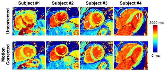
Examples of pre-contrast T1 maps reconstructed before (uncorrected) and after motion correction. Large to severe motion artifacts are visible in all shown T1 maps reconstructed without motion correction. After motion correction, the quality of all T1 maps significantly improved and motion artifacts were substantially reduced.
Figure 9.
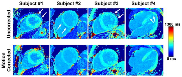
Examples of post-contrast T1 maps reconstructed before (uncorrected) and after motion correction. Motion artifacts are evident in all original (uncorrected) T1 maps (see white arrows). The motion artifact level substantially decreased in motion corrected T1 maps.
Figure 10.
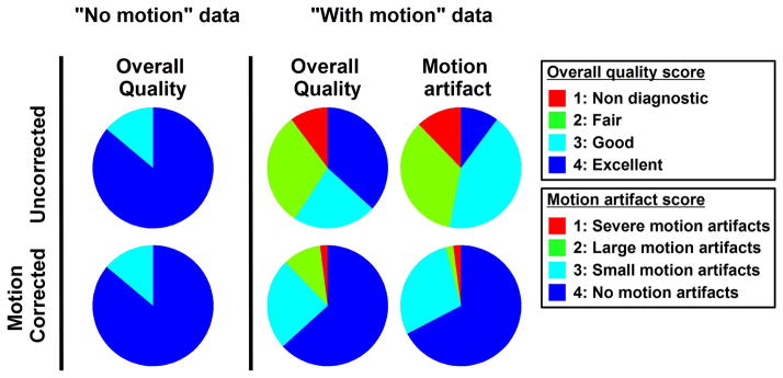
Subjective qualitative analysis of T1 map before (uncorrected) and after motion correction. Similar T1 map quality is observed before and after motion correction in data identified as “no motion”. Improved image quality and reduced motion artifacts were observed after motion correction in data identified as “with motion”.
The computation time of ARCTIC for one T1-weighted image was ~10 seconds using the CPU only implementation and was reduced to ~1 second using the CPU/GPU implementation. Motion estimation and correction of a complete T1 scan using ARCTIC was thus performed in less than 10 seconds using the proposed CPU/GPU implementation.
DISCUSSION
In this study, we proposed a novel motion correction approach for both pre-contrast and post-contrast T1 mapping. The method was successfully validated in a patient cohort. Improved alignment of the myocardium was achieved in all T1-weighted images and all image series assessed as “with motion”. The method did not introduce unrealistic deformation for image series assessed as “no motion”. Furthermore, the proposed motion correction led to significant improvements in overall T1 map quality and substantially reduced the level of motion artifacts. Finally, our CPU/GPU implementation enables the processing of one complete T1 scan in less than 10 seconds which is suitable for clinical applicability.
Motion was observed in 56% of image series which is similar to prior studies which identified motion in 40% (16) and 48% (15) of series. The strong relation between the presence of motion and decreased overall T1 map quality/increased motion artifacts demonstrates that motion is a major challenge for T1 mapping. The significant improvements obtained after motion correction in subjective T1 map assessment shows that the proposed image-registration algorithm represents an efficient strategy to address the motion issue.
DSCs and MBEs measured before motion correction in “no motion” series were found in good agreements with previous studies (15,16). Although the proposed motion correction approach provided a slight improvement in “no motion data”, it did not impact the quality of reconstructed T1 maps as revealed by the subjective qualitative analysis. On the other hand, large DSC increase and MBE reduction were obtained after motion correction in “with motion” data and led to significantly improved T1 maps in term of both overall quality and motion artifacts. This demonstrates the robustness of our approach for both series depicting minimal motion and large amplitude motion. The proposed approach was also found robust for both pre-contrast and post-contrast image series as well as for short axis and four chamber data.
The method was found reliable for all T1-weighted images. However, slightly lower DSCs and higher MBEs were consistently obtained in three post-contrast T1-weighted images (1st, 5th, 8th T1-weighted images) of “no motion” post-contrast data (Figure S1c,e, S2c,e, S3c,e, S4c,e). It appears unlikely that lower DSCs in uncorrected data could be related to any physiological motion since the myocardial motion can generally be characterized in most patients as a drifting motion or a stochastic motion pattern due to RR-interval variations. Drifting motion leads to reduced DSCs in T1-weighted images acquired toward the beginning and the end of the sequence. Stochastic motion pattern should similarly affect all T1-weighted images when analyzed among a sufficiently large cohort. Therefore, it is likely that these reduced DSCs may be related to decrease accuracy in the manual myocardial delineation performed for DSC evaluation. Indeed, with the employed 4-(1)-3-(1)-2 post-contrast MOLLI scheme, these three images are directly acquired after an inversion pulse using a short inversion time. Therefore, the contrast between myocardium, blood and fat is substantially different in those 3 images, and may reduce the accuracy of manual myocardial delineation and may lead to constant under-estimation or over-estimation of the myocardial area. Furthermore, this effect seemed to be more pronounced in four chamber data acquired in patients with large amount of fat, and could occasionally lead to incorrect local motion estimates in images directly acquired after an inversion pulse.
Lower DSCs and higher MBEs were observed in uncorrected “with motion” data acquired during pre-contrast in short axis orientation (Figure 6b and Figure 7b, respectively). This can be mainly explained by the presence of large heart displacements (up to 2 cm) in few pre-contrast image series. Smaller motion patterns (higher DSCs and reduced MBEs) were observed in uncorrected post-contrast data acquired in the same patients. Training effect may explain their improved ability to sustain stable breath-holds during post-contrast imaging. In addition, some patients only underwent pre-contrast imaging which may have also contributed to increase differences between pre-contrast and post-contrast short axis data.
The motion correction approach was tested using the MOLLI T1 mapping technique (12). Therefore, the performance of the method with other T1 mapping sequences such as Shortened MOLLI (ShMOLLI) (13), Saturation recovery single-shot acquisition (SASHA) (11), or SAturation Pulse Prepared Heart rate independent Inversion-REcovery sequence (SAPPHIRE) (14) remains to be investigated. ShMOLLI and MOLLI techniques use multiple Look-Locker experiments (20) with similar inversion time ranges. Therefore, T1-weighted images in ShMOLLI and MOLLI generally depict similar intensity/contrast variation range and it is anticipated to obtain similar motion correction performance with both techniques. SASHA and SAPPHIRE acquisitions use saturation pulses at every heart beat which generally lead to T1-weighted images with reduced intensity/contrast. Therefore, the ability of the ARCTIC method to detect complex motion in those images will need to be carefully evaluated in future studies.
In this study, two approaches were evaluated for the selection of the reference image. Although good registration performance was achieved with the two strategies, the selection of the image with the longest inversion time may offer a more robust and automatic way to use ARCTIC in the presence of alternative acquisition schemes or other T1 mapping sequences.
Respiratory-induced motion and RR-interval variations represent the dominant components of the myocardial deformation/displacement in T1-weighted images. However, patients being imaged during arrhythmic event may show high RR-interval variations which can lead to more complex deformation of the myocardium. Although the elastic nature of the proposed local non-rigid motion estimation was found to successfully account for respiratory-induced motion and RR-interval variations, the robustness of the method in the presence of significant cardiac motion remains to be evaluated. Finally, the proposed method is retrospective and cannot account for through-plane motion. Prospective motion correction using respiratory navigation techniques could be employed to minimize though-plane motion (35). This may also reduce in-plane motion, which would facilitate the image-based registration process. 3D T1 mapping has been recently proposed (36,37) and could be a promising strategy to account for through-plane motion.
The same calibration of the weighting parameters (α,β,λ,R) was used across all patients and all datasets. However, it is likely that personalized parameter calibration may further improve the registration. For example, reduced α values may allow for the estimation of more complex motion while higher α values may improves the robustness of motion estimates against noise (38). Since the noise level and the motion complexity encountered in the myocardium are patient-specific and acquisition-specific, a personalized calibration of the weighting parameters may improve registration performance. Furthermore, the use of robust estimators such as the Lorentzian instead of the L2 norm in the variational formulation of the optical flow problem may reduce the impact of outlier and lead to improved registration (39). This will need to be investigated in future work.
Furthermore, native and post-contrast T1 mapping can be used for automatic ECV measurements, which requires the co-registration of both T1 maps. The co-registration can be performed using the pair of T1-weighted images with longest inversion times (34). These images generally have similar contrast which facilitates the co-registration. The potential of the ARCTIC approach for the co-registration of native and post-contrast T1 maps will be investigated in future studies.
There are several limitations in this study. DICE similarity coefficients were used to quantify the registration. Although it gives a good measure of myocardium alignment, it does not provide a true measure of accuracy. The target registration error (40), which measures the registration error at some points of interest, can be used to accurately quantify the accuracy of a registration approach. This metric requires manual tracking of a set of points across the reference image and the images to be registered. However, due to the lack of anatomical features over the myocardium and the limited intensity/contrast in certain T1-weighted images, point tracking was difficult to achieve and the target registration error was not measured.
CONCLUSIONS
A novel approach has been developed for the correction of respiratory-induced motion occurring during breath-hold T1 mapping sequences. The method provides excellent motion correction for both pre-contrast and post-contrast T1 mapping, and significantly improves the quality of T1 maps.
Supplementary Material
Figure S1. Average DICE similarity coefficient (DSC) of each T1-weighted image obtained in short axis image series. Results are shown for “no motion” image series (a,c,e) and “with motion” image series (b,d,f) as well as different acquisition time point: pre-contrast (a,b), early post contrast (c,d), and late post-contrast (e,f) imaging. Similar DSCs were obtained for each T1-weighted image before and after motion correction in “no motion” image series. DSCs were substantially increased after motion correction in all T1-weighted images of “with motion” image series.
Figure S2. Average DICE similarity coefficient (DSC) of each T1-weighted image obtained in four chamber image series. Results are shown for “no motion” image series (a,c,e) and “with motion” image series (b,d,f) as well as different acquisition time point: pre-contrast (a,b), early post contrast (c,d), and late post-contrast (e,f) imaging. Similar DSCs were obtained for each T1-weighted image before and after motion correction in “no motion” image series. DSCs were substantially increased using ARCTIC for all other T1-weighted images of “with motion” image series.
Figure S3. Average myocardial boundary error (MBE) of each T1-weighted image obtained in short axis image series. Results are shown for “no motion” image series (a,c,e) and “with motion” image series (b,d,f) as well as different acquisition time point: pre-contrast (a,b), early post contrast (c,d), and late post-contrast (e,f) imaging. Similar MBEs were obtained for each T1-weighted image before and after motion correction in “no motion” image series. MBEs were substantially decreased after motion correction in all T1-weighted images of “with motion” image series.
Figure S4. Average myocardial boundary error (MBE) of each T1-weighted image obtained in four chamber image series. Results are shown for “no motion” image series (a,c,e) and “with motion” image series (b,d,f) as well as different acquisition time point: pre-contrast (a,b), early post contrast (c,d), and late post-contrast (e,f) imaging. Similar MBEs were obtained for each T1-weighted image before and after motion correction in “no motion” image series. MBEs were substantially decreased using ARCTIC for most T1-weighted images of “with motion” image series.
Acknowledgments
Supported in part by NIH R01EB008743-01A2.
APPENDIX
The functional EARCTIC(u,v) is minimized using the calculus of variation and by solving the associated Euler-Langrage equations. Using the Laplacian approximation defined as ∇2u = u − ū and ∇2v = v − v̄ with (ū, v̄) the average value of (u, v) in the neighborhood (3×3 pixels) of the estimated point (24), the following system of equations can be obtained:
| [16] |
where , and . This system is solved using the Gauss-Seidel approach which provides the following iterative scheme:
| [17] |
with
| [18] |
References
- 1.Beltrami CA, Finato N, Rocco M, Feruglio GA, Puricelli C, Cigola E, Quaini F, Sonnenblick EH, Olivetti G, Anversa P. Structural basis of end-stage failure in ischemic cardiomyopathy in humans. Circulation. 1994;89(1):151–163. doi: 10.1161/01.cir.89.1.151. [DOI] [PubMed] [Google Scholar]
- 2.Beltrami CA, Finato N, Rocco M, Feruglio GA, Puricelli C, Cigola E, Sonnenblick EH, Olivetti G, Anversa P. The cellular basis of dilated cardiomyopathy in humans. J Mol Cell Cardiol. 1995;27(1):291–305. doi: 10.1016/s0022-2828(08)80028-4. [DOI] [PubMed] [Google Scholar]
- 3.Weber KT, Brilla CG. Pathological hypertrophy and cardiac interstitium. Fibrosis and renin-angiotensin-aldosterone system. Circulation. 1991;83(6):1849–1865. doi: 10.1161/01.cir.83.6.1849. [DOI] [PubMed] [Google Scholar]
- 4.Kim RJ, Wu E, Rafael A, Chen EL, Parker MA, Simonetti O, Klocke FJ, Bonow RO, Judd RM. The use of contrast-enhanced magnetic resonance imaging to identify reversible myocardial dysfunction. N Engl J Med. 2000;343(20):1445–1453. doi: 10.1056/NEJM200011163432003. [DOI] [PubMed] [Google Scholar]
- 5.Simonetti OP, Kim RJ, Fieno DS, Hillenbrand HB, Wu E, Bundy JM, Finn JP, Judd RM. An improved MR imaging technique for the visualization of myocardial infarction. Radiology. 2001;218(1):215–223. doi: 10.1148/radiology.218.1.r01ja50215. [DOI] [PubMed] [Google Scholar]
- 6.Sado DM, Flett AS, Moon JC. Novel imaging techniques for diffuse myocardial fibrosis. Future Cardiol. 2011;7(5):643–650. doi: 10.2217/fca.11.45. [DOI] [PubMed] [Google Scholar]
- 7.Schulz-Menger J, Friedrich MG. Magnetic resonance imaging in patients with cardiomyopathies: when and why. Herz. 2000;25(4):384–391. doi: 10.1007/s000590050030. [DOI] [PubMed] [Google Scholar]
- 8.Arheden H, Saeed M, Higgins CB, Gao DW, Bremerich J, Wyttenbach R, Dae MW, Wendland MF. Measurement of the distribution volume of gadopentetate dimeglumine at echo-planar MR imaging to quantify myocardial infarction: comparison with 99mTc-DTPA autoradiography in rats. Radiology. 1999;211(3):698–708. doi: 10.1148/radiology.211.3.r99jn41698. [DOI] [PubMed] [Google Scholar]
- 9.Iles L, Pfluger H, Phrommintikul A, Cherayath J, Aksit P, Gupta SN, Kaye DM, Taylor AJ. Evaluation of diffuse myocardial fibrosis in heart failure with cardiac magnetic resonance contrast-enhanced T1 mapping. J Am Coll Cardiol. 2008;52(19):1574–1580. doi: 10.1016/j.jacc.2008.06.049. [DOI] [PubMed] [Google Scholar]
- 10.Messroghli DR, Nordmeyer S, Dietrich T, Dirsch O, Kaschina E, Savvatis K, Oh-I D, Klein C, Berger F, Kuehne T. Assessment of diffuse myocardial fibrosis in rats using small-animal Look-Locker inversion recovery T1 mapping. Circ Cardiovasc Imaging. 2011;4(6):636–640. doi: 10.1161/CIRCIMAGING.111.966796. [DOI] [PubMed] [Google Scholar]
- 11.Chow K, Flewitt JA, Green JD, Pagano JJ, Friedrich MG, Thompson RB. Saturation recovery single-shot acquisition (SASHA) for myocardial T1 mapping. Magn Reson Med. 2013 doi: 10.1002/mrm.24878. In Press. [DOI] [PubMed] [Google Scholar]
- 12.Messroghli DR, Radjenovic A, Kozerke S, Higgins DM, Sivananthan MU, Ridgway JP. Modified Look-Locker inversion recovery (MOLLI) for high-resolution T1 mapping of the heart. Magn Reson Med. 2004;52(1):141–146. doi: 10.1002/mrm.20110. [DOI] [PubMed] [Google Scholar]
- 13.Piechnik SK, Ferreira VM, Dall’Armellina E, Cochlin LE, Greiser A, Neubauer S, Robson MD. Shortened Modified Look-Locker Inversion recovery (ShMOLLI) for clinical myocardial T1-mapping at 1. 5 and 3 T within a 9 heartbeat breathhold. J Cardiovasc Magn Reson. 2010;12:69. doi: 10.1186/1532-429X-12-69. [DOI] [PMC free article] [PubMed] [Google Scholar]
- 14.Weingartner S, Akcakaya M, Basha T, Kissinger KV, Goddu B, Berg S, Manning WJ, Nezafat R. Combined saturation/inversion recovery sequences for improved evaluation of scar and diffuse fibrosis in patients with arrhythmia or heart rate variability. Magn Reson Med. 2013 doi: 10.1002/mrm.24761. In Press. [DOI] [PubMed] [Google Scholar]
- 15.Xue H, Greiser A, Zuehlsdorff S, Jolly MP, Guehring J, Arai AE, Kellman P. Phase-sensitive inversion recovery for myocardial T1 mapping with motion correction and parametric fitting. Magn Reson Med. 2013;69(5):1408–1420. doi: 10.1002/mrm.24385. [DOI] [PMC free article] [PubMed] [Google Scholar]
- 16.Xue H, Shah S, Greiser A, Guetter C, Littmann A, Jolly MP, Arai AE, Zuehlsdorff S, Guehring J, Kellman P. Motion correction for myocardial T1 mapping using image registration with synthetic image estimation. Magn Reson Med. 2012;67(6):1644–1655. doi: 10.1002/mrm.23153. [DOI] [PMC free article] [PubMed] [Google Scholar]
- 17.Maintz JB, Viergever MA. A survey of medical image registration. Med Image Anal. 1998;2(1):1–36. doi: 10.1016/s1361-8415(01)80026-8. [DOI] [PubMed] [Google Scholar]
- 18.Makela T, Clarysse P, Sipila O, Pauna N, Pham QC, Katila T, Magnin IE. A review of cardiac image registration methods. IEEE Trans Med Imaging. 2002;21(9):1011–1021. doi: 10.1109/TMI.2002.804441. [DOI] [PubMed] [Google Scholar]
- 19.Nekolla S, Gneiting T, Syha J, Deichmann R, Haase A. T1 maps by K-space reduced snapshot-FLASH MRI. J Comput Assist Tomogr. 1992;16(2):327–332. doi: 10.1097/00004728-199203000-00031. [DOI] [PubMed] [Google Scholar]
- 20.Look DC, Locker DR. Time saving in measurement of NMR and EPR relaxation times. Review of Scientific Instruments. 1970;41(2):250–251. [Google Scholar]
- 21.Rao KR, Hwang JJ. Techniques and standards for image, video, and audio coding. Prentice-Hall, Inc; 1996. [Google Scholar]
- 22.Roujol S, Benois-Pineau J, de Senneville BD, Ries M, Quesson B, Moonen CT. Robust real-time-constrained estimation of respiratory motion for interventional MRI on mobile organs. IEEE Trans Inf Technol Biomed. 2012;16(3):365–374. doi: 10.1109/TITB.2012.2190366. [DOI] [PubMed] [Google Scholar]
- 23.Roujol S, Ries M, Quesson B, Moonen C, Denis de Senneville B. Real-time MR-thermometry and dosimetry for interventional guidance on abdominal organs. Magn Reson Med. 2010;63(4):1080–1087. doi: 10.1002/mrm.22309. [DOI] [PubMed] [Google Scholar]
- 24.Horn BK, Schunck BG. Determining optical flow. Artificial intelligence. 1981;17(1):185–203. [Google Scholar]
- 25.Lucas BD, Kanade T. An iterative image registration technique with an application to stereo vision. 1981:674–679. [Google Scholar]
- 26.Beauchemin SS, Barron JL. The computation of optical flow. ACM Computing Surveys (CSUR) 1995;27(3):433–466. [Google Scholar]
- 27.Cornelius N, Kanade T. Adapting optical-flow to measure object motion in reflectance and x-ray image sequences. ACM SIGGRAPH Computer Graphics. 1984;18(1):24–25. [Google Scholar]
- 28.Kim YS, Lee JH, Ra JB. Multi-sensor image registration based on intensity and edge orientation information. Pattern Recognition. 2008;41(11):3356–3365. [Google Scholar]
- 29.Kellman P, Arai AE, Xue H. T1 and extracellular volume mapping in the heart: estimation of error maps and the influence of noise on precision. J Cardiovasc Magn Reson. 2013;15:56. doi: 10.1186/1532-429X-15-56. [DOI] [PMC free article] [PubMed] [Google Scholar]
- 30.Pratikakis I, Barillot C, Hellier P, Memin E. Robust multiscale deformable registration of 3D ultrasound images. International Journal of Image and Graphics. 2003;3(04):547–565. [Google Scholar]
- 31.Sass M, Ziessow D. Error analysis for optimized inversion recovery spin-lattice relaxation measurements. Journal of Magnetic Resonance (1969) 1977;25(2):263–276. [Google Scholar]
- 32.levmar Lourakis M. [Accessed on June 1, 2013];Levenberg-Marquardt nonlinear least squares algorithms in C/C++ 2004 http://wwwicsforthgr/~lourakis/levmar. Updated on November 29, 2011.
- 33.Dice LR. Measures of the amount of ecologic association between species. Ecology. 1945;26(3):297–302. [Google Scholar]
- 34.Kellman P, Wilson JR, Xue H, Ugander M, Arai AE. Extracellular volume fraction mapping in the myocardium, part 1: evaluation of an automated method. J Cardiovasc Magn Reson. 2012;14:63. doi: 10.1186/1532-429X-14-63. [DOI] [PMC free article] [PubMed] [Google Scholar]
- 35.Wang Y, Riederer SJ, Ehman RL. Respiratory motion of the heart: kinematics and the implications for the spatial resolution in coronary imaging. Magn Reson Med. 1995;33(5):713–719. doi: 10.1002/mrm.1910330517. [DOI] [PubMed] [Google Scholar]
- 36.Clique H, Cheng H, Marie P, Felblinger J, Beaumont M. 3D myocardial T1 mapping at 3T using variable flip angle method. Magn Reson Med. 2013 doi: 10.1002/mrm.24688. In Press. [DOI] [PubMed] [Google Scholar]
- 37.Coniglio A, Di Renzi P, Vilches Freixas G, Della Longa G, Santarelli A, Capparella R, Nardiello B, Loiudice C, Bianchi S, D’Arienzo M, Begnozzi L. Multiple 3D inversion recovery imaging for volume T1 mapping of the heart. Magn Reson Med. 2013;69(1):163–170. doi: 10.1002/mrm.24248. [DOI] [PubMed] [Google Scholar]
- 38.Roujol S, Ries M, Moonen C, de Senneville BD. Automatic nonrigid calibration of image registration for real time MR-guided HIFU ablations of mobile organs. IEEE Trans Med Imaging. 2011;30(10):1737–1745. doi: 10.1109/TMI.2011.2144615. [DOI] [PubMed] [Google Scholar]
- 39.Black MJ, Anandan P. A framework for the robust estimation of optical flow. Proceedings of the Fourth International Conference on Computer Vision: IEEE; 1993; pp. 231–236. [Google Scholar]
- 40.Mandava VR, Fitzpatrick JM, Maurer CR, Jr, Maciunas RJ, Allen GS. Registration of multimodal volume head images via attached markers. Medical Imaging VI: Image Processing. 1992;1652:271–282. [Google Scholar]
Associated Data
This section collects any data citations, data availability statements, or supplementary materials included in this article.
Supplementary Materials
Figure S1. Average DICE similarity coefficient (DSC) of each T1-weighted image obtained in short axis image series. Results are shown for “no motion” image series (a,c,e) and “with motion” image series (b,d,f) as well as different acquisition time point: pre-contrast (a,b), early post contrast (c,d), and late post-contrast (e,f) imaging. Similar DSCs were obtained for each T1-weighted image before and after motion correction in “no motion” image series. DSCs were substantially increased after motion correction in all T1-weighted images of “with motion” image series.
Figure S2. Average DICE similarity coefficient (DSC) of each T1-weighted image obtained in four chamber image series. Results are shown for “no motion” image series (a,c,e) and “with motion” image series (b,d,f) as well as different acquisition time point: pre-contrast (a,b), early post contrast (c,d), and late post-contrast (e,f) imaging. Similar DSCs were obtained for each T1-weighted image before and after motion correction in “no motion” image series. DSCs were substantially increased using ARCTIC for all other T1-weighted images of “with motion” image series.
Figure S3. Average myocardial boundary error (MBE) of each T1-weighted image obtained in short axis image series. Results are shown for “no motion” image series (a,c,e) and “with motion” image series (b,d,f) as well as different acquisition time point: pre-contrast (a,b), early post contrast (c,d), and late post-contrast (e,f) imaging. Similar MBEs were obtained for each T1-weighted image before and after motion correction in “no motion” image series. MBEs were substantially decreased after motion correction in all T1-weighted images of “with motion” image series.
Figure S4. Average myocardial boundary error (MBE) of each T1-weighted image obtained in four chamber image series. Results are shown for “no motion” image series (a,c,e) and “with motion” image series (b,d,f) as well as different acquisition time point: pre-contrast (a,b), early post contrast (c,d), and late post-contrast (e,f) imaging. Similar MBEs were obtained for each T1-weighted image before and after motion correction in “no motion” image series. MBEs were substantially decreased using ARCTIC for most T1-weighted images of “with motion” image series.