Instrumental Variable Analysis with a Nonlinear Exposure–Outcome Relationship

Supplemental Digital Content is available in the text.

Abstract

Background:

Instrumental variable methods can estimate the causal effect of an exposure on an outcome using observational data. Many instrumental variable methods assume that the exposure–outcome relation is linear, but in practice this assumption is often in doubt, or perhaps the shape of the relation is a target for investigation. We investigate this issue in the context of Mendelian randomization, the use of genetic variants as instrumental variables.

Methods:

Using simulations, we demonstrate the performance of a simple linear instrumental variable method when the true shape of the exposure–outcome relation is not linear. We also present a novel method for estimating the effect of the exposure on the outcome within strata of the exposure distribution. This enables the estimation of localized average causal effects within quantile groups of the exposure or as a continuous function of the exposure using a sliding window approach.

Results:

Our simulations suggest that linear instrumental variable estimates approximate a population-averaged causal effect. This is the average difference in the outcome if the exposure for every individual in the population is increased by a fixed amount. Estimates of localized average causal effects reveal the shape of the exposure–outcome relation for a variety of models. These methods are used to investigate the relations between body mass index and a range of cardiovascular risk factors.

Conclusions:

Nonlinear exposure–outcome relations should not be a barrier to instrumental variable analyses. When the exposure–outcome relation is not linear, either a population-averaged causal effect or the shape of the exposure–outcome relation can be estimated.

Most methods for estimating causal effects using instrumental variables (IVs) make the assumption that the relation between the exposure and outcome is linear.¹

Although this may be approximately true in many cases, especially after transforming the exposure or outcome, in some situations, the exposure–outcome relation will be nonlinear. In this case, the shape of the relation may be a target for investigation. For example, the observed relation between body mass index (BMI) and mortality is highly nonlinear, with mortality increasing sharply as BMI increases. However, an increased risk of mortality has also been observed for individuals with low BMI.² It is unclear whether this merely reflects reverse causation (sick people lose weight) or confounding (underweight individuals differ in other risk factors from those of average weight) or whether there is a causal effect of low BMI on increased mortality.³

In a randomized trial where the exposure is the treatment received and the IV is treatment assignment, an IV analysis estimates a local average treatment effect.^4,5

This is the average change in the outcome resulting from a change in the exposure among those patients for whom treatment assignment influences the treatment received. In a trial context, such patients are known as compliers, and the local average treatment effect is also known as a complier-averaged causal effect.⁶ Consistency of the IV estimator is subject to the assumption that any effect of the IV on the exposure is in the same direction for all persons (known as the monotonicity assumption).

In an observational study, the IV and the exposure may be continuous rather than dichotomous. Here, the monotonicity assumption is that the exposure is a nondecreasing function of the IV for all persons (or, equivalently, a nonincreasing function for all persons). This is plausible in the context of Mendelian randomization—the use of genetic variants as IVs—because the biological effects of genetic variants are likely to be in the same direction in each person.⁷ The IV estimate can then be viewed as a weighted average of partial derivatives of the relation of the outcome with the exposure.⁸ In the discrete case, these derivatives can be interpreted as local average treatment effects at different values of the exposure and the IV.

In this study, we explore the implications of nonlinear exposure–outcome relations for IV analyses, particularly in the context of Mendelian randomization. We initially consider the consequences of using linear IV models to estimate the effect of an exposure on an outcome when the true causal relation is nonlinear. We then introduce a novel approach for estimating localized average causal effects, which are IV estimates (local average treatment effects) estimated for strata of the population defined by the value of the exposure. These can provide evidence of a nonlinear effect of the exposure on the outcome. We discuss the findings and implications of our results and compare the approach introduced in this study with other parametric and nonparametric approaches to nonlinear IV analysis. We assume that the exposure and outcome are continuous; issues relating to binary outcomes are reserved for the discussion.

This study is illustrated using data on 8090 subcohort participants from the multicenter case-cohort study European Prospective Investigation into Cancer and Nutrition (EPIC)-InterAct, the diabetes-focused component of the EPIC.⁹ We use data on BMI (kg/m²) and a range of cardiovascular risk factors: systolic blood pressure (mmHg), C-reactive protein (mg/L, log-transformed), uric acid (μmol/L), glycated hemoglobin (HbA1c, %), total cholesterol (mmol/L), and triglycerides (mmol/L, log-transformed). Increases in BMI have been shown to have causal effects on each of these factors in previous Mendelian randomization studies.^10–12 The observational association of each of the risk factors with BMI in a linear regression model, and with BMI and BMI-squared in a quadratic regression model, is given in Table 1. (BMI is centered before analysis, adjustment is made for age, sex, and center.) The mean levels and 95% confidence intervals (CIs) of the risk factors for each quintile of BMI are shown in Figure 1. The observational relations of BMI with several of the risk factors are nonlinear, although this does not necessarily imply that the causal relations will be nonlinear.

TABLE 1.

Coefficients from Observational Analysis of the Association of Body Mass Index (BMI) with a Range of Cardiovascular Risk Factors in Linear and Quadratic Regression Models

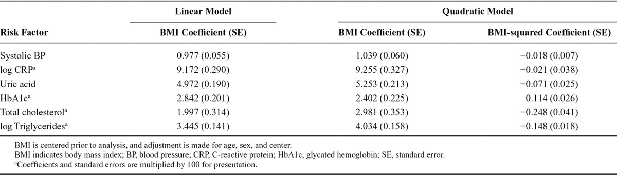
FIGURE 1.

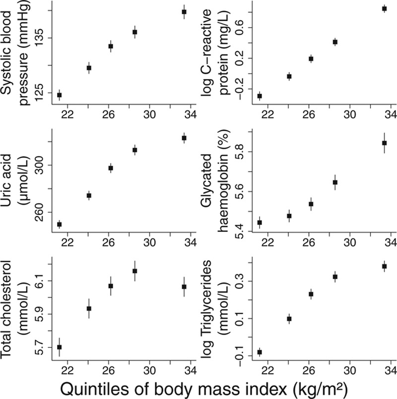
Mean level of cardiovascular risk factors stratified by quintile of body mass index against mean value of body mass index in quintile (lines are ±1.96 standard errors).

LINEAR INSTRUMENTAL VARIABLE ANALYSIS WITH NONLINEAR RELATIONS

It has been suggested that the use of linear models for IV analysis may have some value even if the underlying exposure–outcome model is nonlinear.¹³ We here perform a simulation study to investigate the interpretation of linear IV estimates of nonlinear relations.

Simulation Study

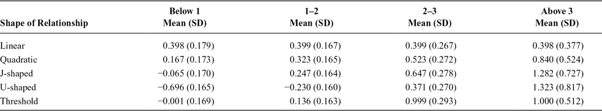
We simulated data for 4000 persons on an IV G, a continuous exposure X taking positive values, a continuous outcome Y, and a confounder U. Five shapes of causal relation were considered between X and Y: a linear relation, a quadratic relation, a J-shaped relation (persons with lower levels of the exposure have slightly increased average outcomes), a U-shaped relation (persons with lower levels of the exposure have considerably increased average outcomes), and a threshold relation. Graphs showing the nonlinear relations between the exposure and mean level of the outcome are given in Figure 2.

FIGURE 2.

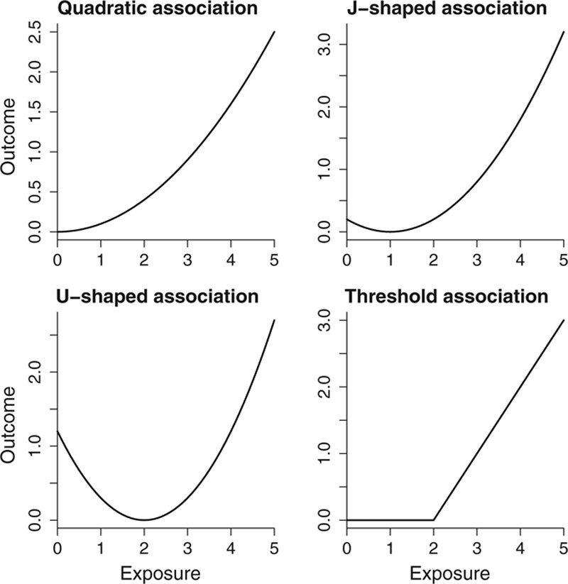
Nonlinear relationships between exposure and outcome for quadratic, J-shaped, U-shaped, and threshold relationship models.

The data-generating model for individual i is:

(1)

where f_j (x_i) is the function associating the exposure and outcome:

The distribution of the IV (G = 0, 1, 2) was chosen to represent the number of variant alleles for a single nucleotide polymorphism with minor allele frequency 0.3. The distribution of the exposure was simulated as positively skewed, with increased values corresponding to greater values of the outcome being less common (95th percentile: 3.7). The IV explained on average 2.4% of the variance in the exposure corresponding to an average F statistic of 49.6. These simulations are repeated in the eAppendix (http://links.lww.com/EDE/A818), altering the data-generating model to allow the effect of the IV on the exposure to vary among individuals and the effect of the exposure on the outcome to vary among individuals.

For each of 10,000 simulated data sets, we calculated the ratio IV estimate (also called the Wald estimate) for the causal effect of the exposure on the outcome.¹⁴ This is calculated as the coefficient for the association of the IV with the outcome divided by the coefficient for the association of the IV with the exposure. For functions f₂ to f₅, the effect of a fixed increase in the exposure differs across the distribution of the exposure. Therefore, we considered the average effects on the outcome of 2 interventions in the exposure: first, to increase the exposure for every individual by 1 unit; and second, to increase the exposure in every individual in the population by 0.25 units (the effect of a unit increase in the IV on the exposure). These quantities have been called population-averaged causal effects¹⁵ or average partial effects,¹⁶ as they average not only across individuals but also across the distribution of the exposure. As the data are simulated, the corresponding outcomes at these counterfactual values of the exposure can be calculated for each individual person.

Results

We present the mean values across simulations of the ratio IV estimate for a 1-unit increase in the exposure, a scaled ratio estimate for a 0.25-unit increase in the exposure, and the mean values of the average changes in the outcome (population-averaged causal effects) for 1-unit and 0.25-unit increases in the exposure (Table 2). Similar results were observed when the effects of the IV on the exposure and of the exposure on the outcome were allowed to vary among individual persons (eAppendix, eTables 1, 3, and 5, http://links.lww.com/EDE/A818).

TABLE 2.

Mean Values Across Simulations of the Ratio Instrumental Variable Estimate Assuming a Linear Exposure–Outcome Relationship and the Population-averaged Causal Effect for 1-unit and 0.25-unit Increases in the Exposure

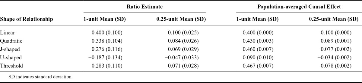
In the linear case, the ratio estimates scaled to a 1-unit and a 0.25-unit increase in the exposure were both equal to the corresponding population-averaged causal effect. In the nonlinear cases, the population-averaged causal effect was similar to the ratio estimate for a 0.25-unit increase but was considerably different for a 1-unit increase. This difference is especially apparent for the U-shaped relation, where a 0.25-unit increase in the exposure led to a fall in the average level of the outcome, but a 1-unit increase led to a rise. Although the approximate equality may not hold for extreme shapes of the exposure–outcome relation, in the examples presented, the ratio IV estimate is close to the population-averaged causal effect for an increase in the exposure distribution of similar size to that associated with a change in the IV if the increase is small. We provide a theoretical motivation for this finding in the eAppendix (http://links.lww.com/EDE/A818). Previous theoretical results have been derived relating the linear IV estimate to a weighted average of derivatives⁸; this finding is similarly motivated, but the interpretation as a population-averaged causal effect is likely to be more familiar to an audience of applied researchers.

In general, the population-averaged causal effect cannot be generalized to the effect of an increase in the exposure for an individual.¹⁷ Even in the linear case, under heterogeneity in the exposure–outcome model, the ratio estimate represents an average causal effect across the population.¹⁸ In the nonlinear case (such as with the threshold relation), a large proportion of the population will have no increase in the outcome associated with a small increase in the exposure, as the increased exposure will not exceed the threshold level. With the J-shaped and U-shaped relations, a small increase in the exposure will lead to increases in the outcome for some persons and decreases for others.

POSSIBLE APPROACHES TO NONLINEAR INSTRUMENTAL VARIABLE ANALYSIS

Although in some cases ignoring any nonlinearity in the exposure–outcome relation and estimating a population-averaged causal effect may be sufficient, doing so does not give the investigator any insight into the shape of the relation. We discuss why standard IV approaches are not generally useful for investigating the shape of nonlinear relations, and we introduce a novel method for the estimation of localized average causal effects at different levels of the exposure distribution.

Unsuitability of Instrumental Variable Approaches for Estimating Nonlinear Relations

When values across the range of the distribution of BMI are compared, there is heterogeneity in the association between BMI and mortality. For example, in an observational setting, comparisons are commonly made and nonlinearities observed between groups of persons with BMI (kg/m²) in the ranges below 18.5 (underweight), 18.5 to 25 (normal weight), 25 to 30 (overweight), and over 30 (obese). In contrast, taking the genetic variant with the greatest association with BMI in the EPIC-InterAct data set (rs1421085, a variant in the FTO gene, R² = 0.39%), persons with no BMI-increasing alleles (major homozygotes) have an average BMI of 26.3, those with 1 allele (heterozygotes) an average BMI of 26.7, and those with 2 alleles (minor homozygotes) an average BMI of 27.1 (Figure 3). Thus, although an observational analysis can compare groups of persons with nonoverlapping distributions of BMI and marked differences in their average BMI values (standard deviation of BMI = 4.33), a standard IV analysis using rs1421085 compares groups of persons with overlapping distributions of BMI and slight differences in their average BMI values (standard deviation of fitted values of BMI conditional on IV = 0.26).

FIGURE 3.

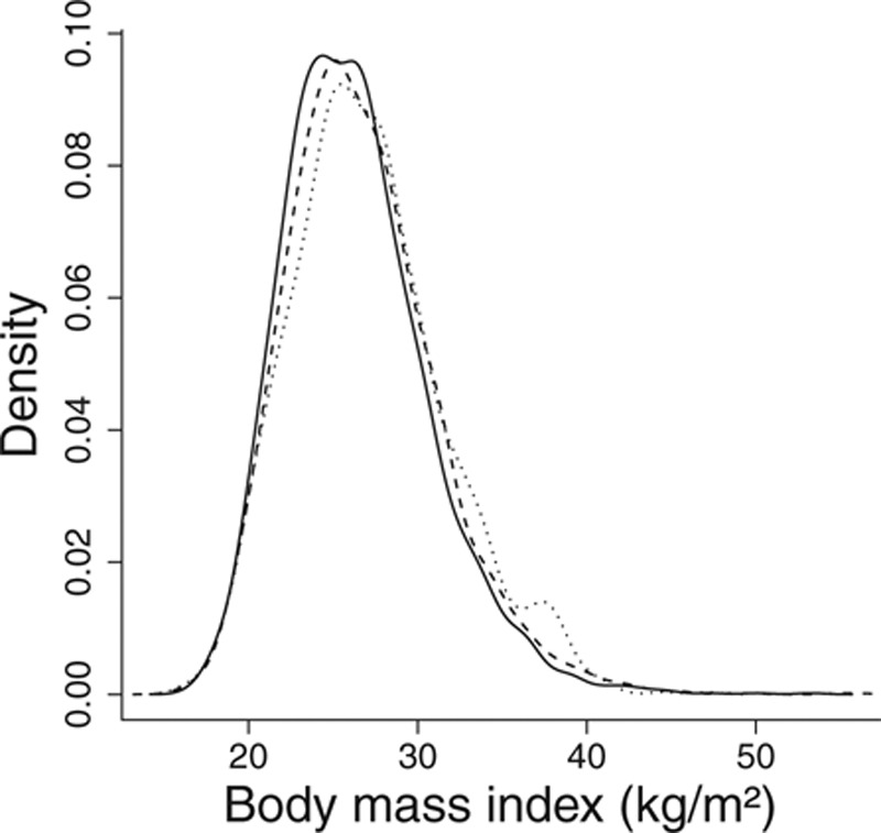
Distribution of body mass index in subgroups defined by genetic variant rs1421085: solid line, major homozygotes; dashed line, heterozygotes; dotted line, minor homozygotes. Densities are smoothed using a kernel-density method with a common bandwidth of 0.8.

Although approaches have been proposed for nonlinear IV analysis,^19–22 information for estimating the effect of the exposure on the outcome is available (without additional assumptions) only for predicted values of exposure based on the IV. Nonlinearity for this reduced range of the exposure distribution is unlikely to be observed. Moreover, this range does not increase as the sample size increases. The shape of the relation outside this range can be estimated by the specification of a parametric model for the exposure–outcome relation; however, inference based on such models has been shown to be highly sensitive to the choice of parametrization.^16,22 We consider these issues further in relation to specific nonparametric IV methods in the discussion.

Stratification of the Exposure and Localized Average Causal Effects

Rather than estimating a population-averaged causal effect, we may wish to estimate an average causal effect for a stratum of the exposure distribution. These localized average causal effects will be constant in expectation if the relation is linear but will give insight into the shape of the exposure–outcome relation if it is nonlinear. As the IV is associated with the exposure, by stratifying on the exposure distribution, an association between the IV and outcome may be induced even if this was not present in the original data.²³ This can be avoided by stratifying based on the residual variation in the exposure conditional on the IV. Under the assumption that there is no heterogeneity in the average effect of the IV on the exposure at different levels of the exposure, this is equivalent to subtracting the effect of the IV from the exposure, and then stratifying individuals based on their IV-free exposure level. The IV-free exposure level represents the expected value of the exposure, which would be observed if a person’s IV value was zero. Although the IV-free exposure may appear to have a counterfactual interpretation, it is not intended to be a counterfactual variable. Rather, it is a function of the observed data. A counterfactual interpretation would require the stronger assumption that the effect of the IV on the exposure was constant for all individuals and is only necessary for the variable that is contrasted in the causal effect and not for the IV-free exposure that takes the role of a stratifying covariate.

Using the same simulated data sets as in the previous section, we stratified individuals based on their IV-free exposure using categories below 1, 1 to 2, 2 to 3, and above 3. For each of these groups, we estimated the (stratum-specific) localized average causal effect of the exposure on the outcome using the ratio method (the association of the IV with the outcome in the stratum divided by the association of the IV with the exposure in the population). The IV-free exposure was calculated based on the estimated value of the association of the IV with the exposure in the whole population. Table 3 shows that the true shape of the exposure–outcome relation is apparent from comparing the mean values of these effects across the simulated data sets.

TABLE 3.

Mean Values Across Simulations of the Localized Average Causal Effects of the Exposure on the Outcome Within Strata Defined by the IV-free Exposure Level

We emphasize the importance of stratifying based on the IV-free exposure; when the same effects were estimated across strata of the exposure without prior subtraction of the effect of the IV, in the linear case, the corresponding estimates were −0.150, −0.052, −0.001, and −0.003. In the directed acyclic graph of Figure 4, conditioning on the exposure X induces an association between G and U, which are both parents of X (termed moralization). In contrast, conditioning on the IV-free exposure X₀ = X − α_GG does not induce such an association.

FIGURE 4.

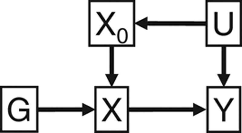
Directed acyclic graph of relationships among instrumental variable (IV) G, exposure X, IV-free exposure X₀, confounder U, and outcome Y.

We calculated Cochran’s Q statistic to examine possible heterogeneity in the 4 estimates. This nonparametric test assesses whether differences between the estimates in the strata are more different than would be expected by chance. We also conducted a trend test by performing a meta-regression of the estimates on the mean values of the exposure in each stratum. This is a form of weighted regression where the variance of each value of the response variable is assumed to be known.²⁴ The proportions of data sets where the Cochran’s Q test rejected the null hypothesis (P < 0.05) were as follows: linear 5.2%, quadratic 25.2%, J-shaped 67.0%, U-shaped 94.7%, and threshold 85.8%. The same proportions for the trend test were linear 4.1%, quadratic 31.8%, J-shaped 73.9%, U-shaped 94.7%, and threshold 65.6%. Similar results were observed when the effects of the IV on the exposure and of the exposure on the outcome were allowed to vary among persons provided that the effect heterogeneities in the IV–exposure and exposure–outcome associations were not correlated (eAppendix, eTables 2, 4, 6, and 7, http://links.lww.com/EDE/A818). We conclude, based on this simulation example, that the heterogeneity and trend tests are at least sometimes able to detect nonlinearities in causal relations. The trend test has greater empirical power to detect nonlinearities, except for in the case of the threshold relation.

A generalization of this approach is to estimate the localized average causal effect across the distribution of the IV-free exposure using a sliding window. This is performed by first ordering individuals according to their IV-free exposure. Using an example window size of 1,000, the localized average causal effect is estimated for the first 1000 people, then for the individuals numbered 2 through to 1,001, then 3 to 1,002, and so on. The estimates can then be plotted against the median exposure value for each window. The range of the exposure distribution over which the localized average causal effect is estimated depends on the window size; however, for a fixed window size, the range expands as the sample increases. In the next section, we explore the impact of the choice of how wide to make the sliding window in a real data example.

APPLIED EXAMPLE: EFFECT OF BODY MASS INDEX ON CARDIOVASCULAR RISK FACTORS

In this section, we apply the linear and localized IV methods to the EPIC-InterAct data set for the cardiovascular risk factors previously listed. Data were available on 29 genetic variants previously shown to be associated with BMI in a large meta-analysis.²⁵ Details of the variants are given in the eAppendix (http://links.lww.com/EDE/A818) and their plausibility as IVs assessed by overidentification tests in each center (eTable 8, http://links.lww.com/EDE/A818). An allele score comprising all the variants weighted by their reported association with BMI in the meta-analysis is used as an IV.²⁶ If an individual i has g_ik copies of variant allele k, that person’s allele score is , where w_k is the weight of the kth variant. The score explains 0.77% of the variance in BMI.

For each outcome, we fit a linear IV model using the ratio method, adjusting for age, sex, and center in the regressions of the outcome on the allele score and of the exposure on the allele score. We estimated the localized average causal effects of BMI on each risk factor within quintiles of the distribution of BMI after the genetic component is subtracted (the IV-free BMI) and performed heterogeneity and trend tests on these values (Table 4). To account for the multiple centers, we standardized the BMI measure used to stratify the data by regressing BMI on age, sex, center, and allele score and stratifying individuals based on their residual value from this regression. Again, adjustment was made in the estimation of the causal effects for age, sex, and center. A more general sliding window approach was also used for estimating localized average causal effects, initially for HbA1c, and then for all the outcomes. Figure 5 displays the estimates for HbA1c using window sizes of 500, 1,000, 1,500, 2,000, 3,000, and 4,000. Figure 6 displays the estimates for all the outcomes using a window size of 2,000. For interpretability, the x-axis is the unstandardized BMI value corresponding to the BMI of the individual in the middle of the window. Previous work has shown that genetic associations with BMI are similar in extremely overweight individuals to those in the general population.²⁷ To assess the assumption that the effect of the IV on BMI is similar across the exposure distribution, we estimated the association of the allele score with BMI in each of the quintiles of IV-free BMI. The association estimates were 0.80, 1.02, 1.02, 0.98, 1.07; standard errors 0.08, 0.03, 0.03, 0.04, 0.19; heterogeneity test P = 0.11; trend test P = 0.26. There is not sufficient evidence in this data set to reject this assumption.

TABLE 4.

Linear IV Estimates of BMI on Risk Factor Outcome from Ratio Method; Localized Average Causal Effect Estimates of BMI on Each Risk Factor Within Quintiles of Participants Stratified by Their IV-free BMI; P Values for Heterogeneity (pQ) and Trend (p_tr) of Estimates

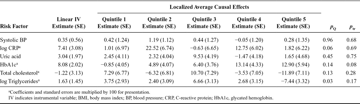
FIGURE 5.

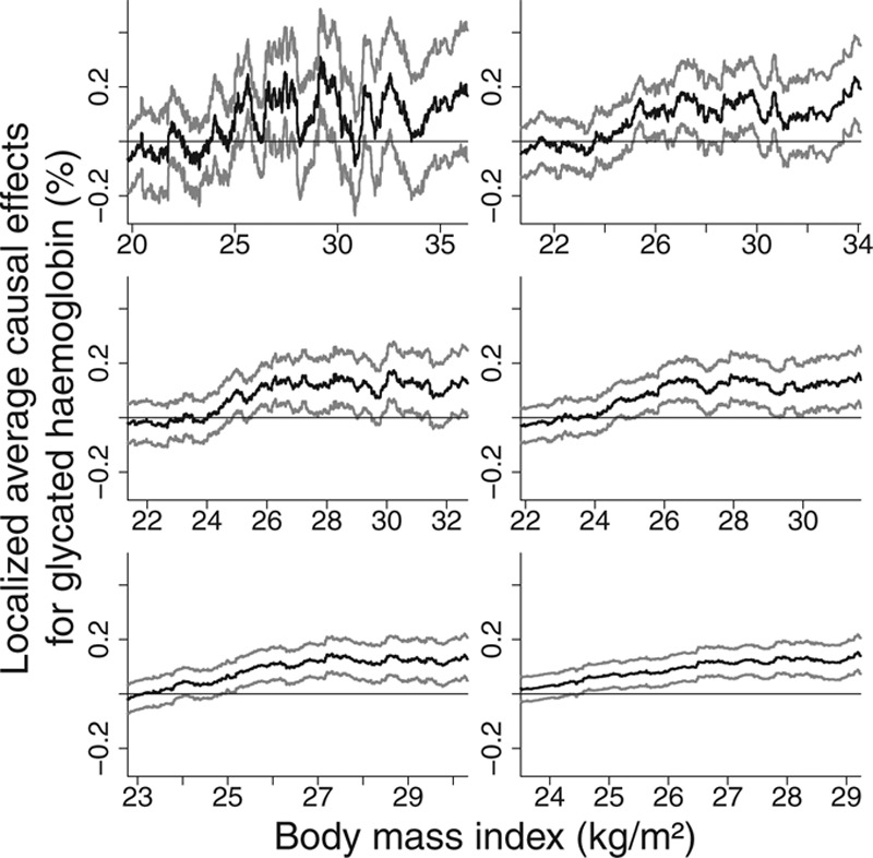
Localized average causal effect estimates of body mass index on glycated hemoglobin at various levels of body mass index from EPIC-InterAct data set: sliding window approach with window sizes 500, 1,000, 1,500, 2,000, 3,000, and 4,000 (top-left to bottom-right). Gray lines represent point wise 95% CIs.

FIGURE 6.

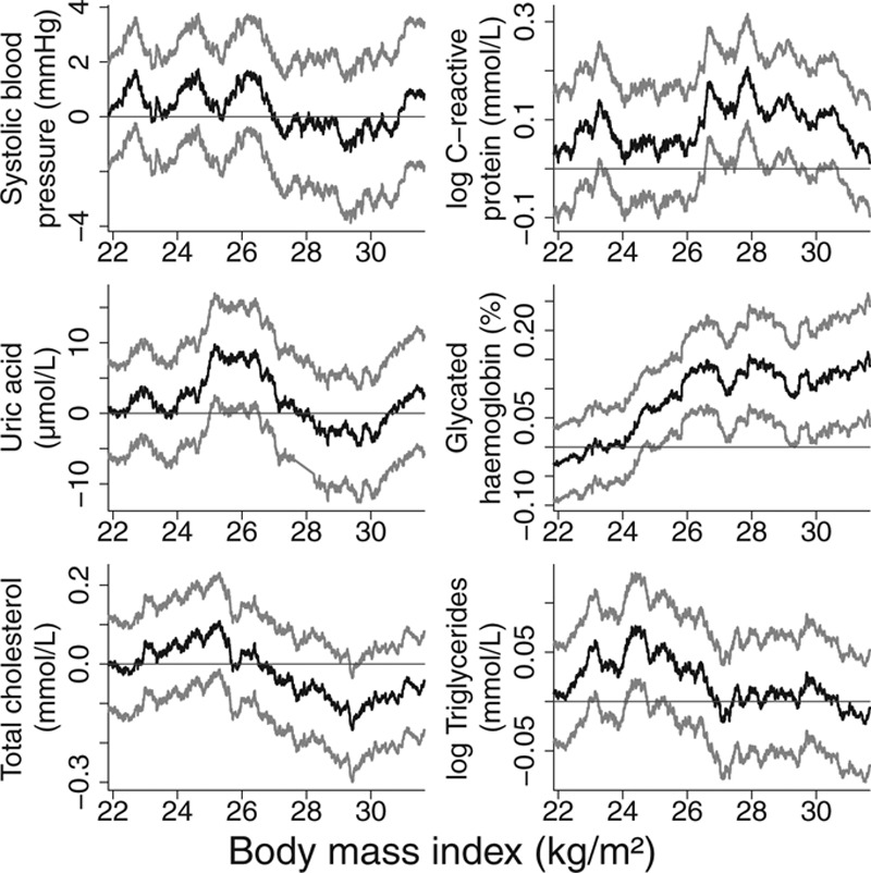
Localized average causal effect estimates of body mass index on cardiovascular risk factors at various levels of body mass index from EPIC-InterAct data set: sliding window approach with window size 2,000. Gray lines represent point wise 95% CIs.

The graphs showing localized average causal effect estimates for HbA1c demonstrate the trade-off in choosing a window size (Figure 5). With a smaller window size, there is increased detail in the estimate of the shape of the exposure–outcome relation and estimates are obtained across a wider range of the exposure distribution. With a larger window size, precision of the estimates is increased. However, the possible threshold feature of the model, whereby the causal estimate is close to zero for low values of BMI, is lost as the window size increases. In addition, the shape of the graphs becomes closer to a straight line. It seems likely that much of the variability in the estimates with a small window size reflects random fluctuation rather than interesting information, hence the use of a moderately large window size in Figure 6. Estimates for total cholesterol and triglycerides show a similar pattern, with positive point estimates for median BMI levels less than 26, and estimates around or below zero for median BMI greater than 28. Larger sample sizes are required for more definitive applied conclusions.

DISCUSSION

In this study, we have discussed the prospects for IV analyses with a nonlinear exposure–outcome relation. Specifically, we have provided an interpretation of linear IV estimates in the presence of nonlinearity and have proposed a novel method to investigate whether causal effects depend on the level of the exposure.

Linear Estimation Approach

Simple linear IV estimators with a nonlinear exposure–outcome relation estimate a parameter that approximates a population-averaged causal effect. This is the average effect resulting from an uniform increase in the exposure for all persons in the population. However, the approximation may be poor for an IV with a large effect on the exposure and will break down if the population-averaged causal effect is considered for a change in the exposure much greater than that associated with the IV. If the exposure–outcome relation is monotonic (i.e., increasing or decreasing in the outcome for all values of the exposure), then the parameter estimated by a linear IV method will be in the same direction as the causal effect for each individual in the population. Nonlinear exposure–outcome relations should therefore not be seen as a barrier to IV analyses, such as Mendelian randomization investigations. However, if the exposure–outcome relation is not monotonic, a causal effect of the exposure on the outcome may be obscured by a linear IV estimate (potentially such as in the applied example of the effect of BMI on log triglycerides).

Parametric and Nonparametric Approaches

If the shape of the exposure–outcome relation is the subject of investigation, then a nonlinear parametric or nonparametric IV analysis can be performed. Inference from nonlinear parametric models has been previously shown to be sensitive to the choice of parametric model in a range of real scenarios.²² Inference from nonparametric models is limited when the IV does not explain much of the variation in the exposure. For example, the series method of Newey and Powell¹⁹ is a 2-stage nonparametric IV method. The first stage constructs a basis set of nonlinear functions (such as a set of orthogonal polynomials or B-splines) of the exposure conditional on the IV, and the second stage fits the outcome as a linear combination of these nonlinear functions. These estimates will not be reliable outside the range of the fitted values of the exposure conditional on the IV. Similar arguments can be made for the kernel and series methods of Hall and Horowitz.²⁰

An alternative approach to nonlinear IV analysis is the quantile regression approach of Chernozhukov and Hansen.²¹ In this case, the identifying assumption of the method is that the unmeasured confounders can be represented by a single variable that has a monotone effect on the outcome.²⁸ This assumption is not only restrictive and unrealistic but also inherently unverifiable, and even sensitivity analyses to investigate the assumption cannot be performed. Such assumptions should not be relied on for identifying causal effects.

Localized Estimation Approach

By stratifying the population based on the IV-free exposure, localized average causal effects of the exposure on the outcome in each of the strata can reveal the shape of the exposure–outcome relation. In practice, such estimates in the strata may be imprecise, meaning that the true shape of the relation is obscured. This approach can be extended using a sliding window approach to provide a continuous estimate of the exposure–outcome relation across a wide range of the exposure distribution.

Unlike with other nonparametric IV approaches, this range widens as the sample size increases. Either stratum-specific or sliding window estimates can equally be estimated with a binary outcome by using a log-linear or logistic analysis model to estimate a relative risk or odds ratio parameter. A localized average causal effect is simply an IV estimate estimated for a particular stratum of the population as defined by the IV-free exposure. The same provisos about the approximation of an IV estimate to a population-averaged causal effect being valid only for small changes in the exposure and for IVs with a small effect on the exposure therefore apply equally for localized average causal effects.

Measurement Error

In observational analyses, coefficients in a linear regression model are affected by regression dilution bias if the exposure suffers from classical measurement error (ie, error uncorrelated with the true value of the exposure).²⁹ Estimates of the shape of nonlinear exposure–outcome relations can be distorted.³⁰ In contrast, IV estimates under such an error model are unbiased.³¹ In the same way, since localized average causal effects are IV estimates for a given stratum of the population, the shape of relation estimated in a localized IV analysis will not be affected by classical measurement error in the exposure.

ACKNOWLEDGMENTS

We thank all EPIC participants and staff for their contribution to the study. We thank staff from the Technical, Field Epidemiology and Data Functional Group Teams of the MRC Epidemiology Unit in Cambridge, UK, for carrying out sample preparation, DNA provision and quality control, genotyping and data-handling work. The EPIC-InterAct study received funding from the European Union (Integrated Project LSHM-CT-2006-037197 in the Framework Programme 6 of the European Community).

REFERENCES

- 1.Herńan M, Robins J. Instruments for causal inference: an epidemiologist’s dream? Epidemiology. 2006;17:360–372. doi: 10.1097/01.ede.0000222409.00878.37. [DOI] [PubMed] [Google Scholar]
- 2.Flegal KM, Kit BK, Orpana H, Graubard BI. Association of all-cause mortality with overweight and obesity using standard body mass index categories: a systematic review and meta-analysis. JAMA. 2013;309:71–82. doi: 10.1001/jama.2012.113905. [DOI] [PMC free article] [PubMed] [Google Scholar]
- 3.Allison DB, Faith MS, Heo M, Kotler DP. Hypothesis concerning the U-shaped relation between body mass index and mortality. Am J Epidemiol. 1997;146:339–349. doi: 10.1093/oxfordjournals.aje.a009275. [DOI] [PubMed] [Google Scholar]
- 4.Imbens GW, Angrist JD. Identification and estimation of local average treatment effects. Econometrica. 1994;62:467–475. [Google Scholar]
- 5.Angrist J, Imbens G, Rubin D. Identification of causal effects using instrumental variables. JAMA. 1996;91:444–455. [Google Scholar]
- 6.Little RJ, Rubin DB. Causal effects in clinical and epidemiological studies via potential outcomes: concepts and analytical approaches. Annu Rev Public Health. 2000;21:121–145. doi: 10.1146/annurev.publhealth.21.1.121. [DOI] [PubMed] [Google Scholar]
- 7.Davey Smith G, Ebrahim S. ‘Mendelian randomization’: can genetic epidemiology contribute to understanding environmental determinants of disease? Int J Epidemiol. 2003;32:1–22. doi: 10.1093/ije/dyg070. [DOI] [PubMed] [Google Scholar]
- 8.Angrist J, Graddy K, Imbens G. The interpretation of instrumental variables estimators in simultaneous equations models with an application to the demand for fish. Rev Econ Stud. 2000;67:499–527. [Google Scholar]
- 9.Langenberg C, Sharp S, Forouhi N, et al. Design and cohort description of the InterAct Project: an examination of the interaction of genetic and lifestyle factors on the incidence of type 2 diabetes in the EPIC Study. Diabetologia. 2011;54:2272–2282. doi: 10.1007/s00125-011-2182-9. [DOI] [PMC free article] [PubMed] [Google Scholar]
- 10.Freathy RM, Timpson NJ, Lawlor DA, et al. Common variation in the FTO gene alters diabetes-related metabolic traits to the extent expected given its effect on BMI. Diabetes. 2008;57:1419–1426. doi: 10.2337/db07-1466. [DOI] [PMC free article] [PubMed] [Google Scholar]
- 11.Fall T, Hägg S, Mägi R, et al. The role of adiposity in cardiometabolic traits: a Mendelian randomization analysis. PLoS Med. 2013;10:e1001 474. doi: 10.1371/journal.pmed.1001474. [DOI] [PMC free article] [PubMed] [Google Scholar]
- 12.Palmer TM, Nordestgaard BG, Benn M, et al. Association of plasma uric acid with ischaemic heart disease and blood pressure: Mendelian randomisation analysis of two large cohorts. BMJ. 2013;347:f4262. doi: 10.1136/bmj.f4262. [DOI] [PMC free article] [PubMed] [Google Scholar]
- 13.Angrist J, Pischke JS. The credibility revolution in empirical economics: how better research design is taking the con out of econometrics. J Econ Pers. 2010;24:3–30. [Google Scholar]
- 14.Didelez V, Meng S, Sheehan N. Assumptions of IV methods for observational epidemiology. Stat Sci. 2010;25:22–40. [Google Scholar]
- 15.Burgess S CHD CRP Genetics Collaboration. Identifying the odds ratio estimated by a two-stage instrumental variable analysis with a logistic regression model. Stat Med. 2013;32:4726–4747. doi: 10.1002/sim.5871. [DOI] [PMC free article] [PubMed] [Google Scholar]
- 16.Mogstad M, Wiswall M. Linearity in instrumental variables estimation: problems and solutions. Technical Report, Forschungsinstitut zur Zukunft der Arbeit. 2010 [Google Scholar]
- 17.Heckman JJ, Vytlacil E. Policy-relevant treatment effects. Am Econ Rev. 2001;91:107–111. [Google Scholar]
- 18.Angrist JD, Imbens GW. Two-stage least squares estimation of average causal effects in models with variable treatment intensity. J Am Stat Assoc. 1995;90:431–442. [Google Scholar]
- 19.Newey WK, Powell JL. Instrumental variable estimation of nonparametric models. Econometrica. 2003;71:1565–1578. [Google Scholar]
- 20.Hall P, Horowitz JL. Nonparametric methods for inference in the presence of instrumental variables. Ann Stat. 2005;33:2904–2929. [Google Scholar]
- 21.Chernozhukov V, Hansen C. An IV model of quantile treatment effects. Econometrica. 2005;73:245–261. [Google Scholar]
- 22.Horowitz JL. Applied nonparametric instrumental variables estimation. Econometrica. 2011;79:347–394. [Google Scholar]
- 23.Didelez V, Sheehan N. Mendelian randomization as an instrumental variable approach to causal inference. Stat Methods Med Res. 2007;16:309–330. doi: 10.1177/0962280206077743. [DOI] [PubMed] [Google Scholar]
- 24.Thompson S, Sharp S. Explaining heterogeneity in meta-analysis: a comparison of methods. Stat Med. 1999;18:2693–2708. doi: 10.1002/(sici)1097-0258(19991030)18:20<2693::aid-sim235>3.0.co;2-v. [DOI] [PubMed] [Google Scholar]
- 25.Speliotes EK, Willer CJ, Berndt SI, et al. Association analyses of 249,796 individuals reveal 18 new loci associated with body mass index. Nat Genet. 2010;42:937–948. doi: 10.1038/ng.686. [DOI] [PMC free article] [PubMed] [Google Scholar]
- 26.Burgess S, Thompson S. Use of allele scores as instrumental variables for Mendelian randomization. Int J Epidemiol. 2013;42:1134–1144. doi: 10.1093/ije/dyt093. [DOI] [PMC free article] [PubMed] [Google Scholar]
- 27.Paternoster L, Evans DM, Nohr EA, et al. Genome-wide population-based association study of extremely overweight young adults—the GOYA study. PLoS One. 2011;6:e24 303. doi: 10.1371/journal.pone.0024303. [DOI] [PMC free article] [PubMed] [Google Scholar]
- 28.Chernozhukov V, Hansen C. Instrumental variable quantile regression: a robust inference approach. J Econ. 2008;142:379–398. [Google Scholar]
- 29.Frost C, Thompson S. Correcting for regression dilution bias: comparison of methods for a single predictor variable. J Royal Stat Soc A. 2000;163:173–189. [Google Scholar]
- 30.Keogh RH, Strawbridge AD, White I. Effects of classical exposure measurement error on the shape of exposure–disease associations. Epidemiol Methods. 2012;1:13–32. [Google Scholar]
- 31.Pierce BL, VanderWeele TJ. The effect of non-differential measurement error on bias, precision and power in Mendelian randomization studies. Int J Epidemiol. 2012;41:1383–1393. doi: 10.1093/ije/dys141. [DOI] [PubMed] [Google Scholar]
- 32.Johnson A, Handsaker R, Pulit S, Nizzari M, O’Donnell C, de Bakker P. SNAP: a web-based tool for identification and annotation of proxy SNPs using HapMap. Bioinformatics. 2008;24:2938–2939. doi: 10.1093/bioinformatics/btn564. [DOI] [PMC free article] [PubMed] [Google Scholar]
- 33.Baum C, Schaffer M, Stillman S. Instrumental variables and GMM: estimation and testing. Stata J. 2003;3:1–31. [Google Scholar]
- 34.Glymour M, Tchetgen Tchetgen E, Robins J. Credible Mendelian randomization studies: approaches for evaluating the instrumental variable assumptions. Am J Epidemiol. 2012;175:332–339. doi: 10.1093/aje/kwr323. [DOI] [PMC free article] [PubMed] [Google Scholar]