Data smashing: uncovering lurking order in data

Abstract

From automatic speech recognition to discovering unusual stars, underlying almost all automated discovery tasks is the ability to compare and contrast data streams with each other, to identify connections and spot outliers. Despite the prevalence of data, however, automated methods are not keeping pace. A key bottleneck is that most data comparison algorithms today rely on a human expert to specify what ‘features' of the data are relevant for comparison. Here, we propose a new principle for estimating the similarity between the sources of arbitrary data streams, using neither domain knowledge nor learning. We demonstrate the application of this principle to the analysis of data from a number of real-world challenging problems, including the disambiguation of electro-encephalograph patterns pertaining to epileptic seizures, detection of anomalous cardiac activity from heart sound recordings and classification of astronomical objects from raw photometry. In all these cases and without access to any domain knowledge, we demonstrate performance on a par with the accuracy achieved by specialized algorithms and heuristics devised by domain experts. We suggest that data smashing principles may open the door to understanding increasingly complex observations, especially when experts do not know what to look for.

1. Introduction

Any experienced data analyst knows that simply feeding raw data directly into a data analysis algorithm is unlikely to produce meaningful results. Most data analysis today involves a substantial and often laborious preprocessing stage, before standard algorithms can work effectively. In this preprocessing stage, data are filtered and reduced into ‘features' that are defined and selected by experts who know what aspects of the data are important, based on extensive domain knowledge.

Relying on experts, however, is slow, expensive, error prone and unlikely to keep pace with the growing amounts and complexity of data. Here, we propose a general way to circumvent the reliance on human experts, with relatively little compromise to the quality of results. We discovered that all ordered datasets—regardless of their origin and meaning—share a fundamental universal structure that can be exploited to compare and contrast them without a human-dependent preprocessing step. We suggest that this process, which we call data smashing, may open the door to understanding increasingly complex data in the future, especially when experts cannot keep pace.

Our key observation, presented here, is that all quantitative data streams have corresponding anti-streams, which in spite of being non-unique, are tied to the stream's unique statistical structure. We then describe the data smashing process by which streams and anti-streams can be algorithmically collided to reveal differences that are difficult to detect using conventional techniques. We establish this principle formally, describe how we implemented it in practice and report its performance on a number of real-world cases from varied disciplines. The results show that without access to any domain knowledge, the unmodified data smashing process performs on a par with specialized algorithms devised by domain experts for each problem independently. For example, we analyse raw electro-encephalographic (EEG) data, and without any domain knowledge find that the measurements from different patients fall into a single curve, with similar pathologies clustered alongside each other. Making such a discovery using conventional techniques would require substantial domain knowledge and data preprocessing (see figure 3a(ii)).

Figure 3.

Data smashing applications. Pairwise distance matrices, identified clusters and three-dimensional projections of Euclidean embeddings for epileptic pathology identification (a), identification of heart murmur (b) and classification of variable stars from photometry (c). In these applications, the relevant clusters are found unsupervised. (Online version in colour.)

2. Anti-streams

The notion of data smashing applies only to data in the form of an ordered series of digits or symbols, such as acoustic waves from a microphone, light intensity over time from a telescope, traffic density along a road or network activity from a router. An anti-stream contains the ‘opposite’ information from the original data stream and is produced by algorithmically inverting the statistical distribution of symbol sequences appearing in the original stream. For example, sequences of digits that were common in the original stream will be rare in the anti-stream, and vice versa. Streams and anti-streams can then be algorithmically ‘collided’ in a way that systematically cancels any common statistical structure in the original streams, leaving only information relating to their statistically significant differences. We call this the principle of information annihilation.

Data smashing involves two data streams and proceeds in three steps (see figure 1): raw data streams are first quantized, by converting continuous value to a string of characters or symbols. The simplest example of such quantization is where all positive values are mapped to the symbol ‘1’ and all negative values to ‘0’, thus generating a string of bits. Next, we select one of the quantized input streams and generate its anti-stream. Finally, we smash this anti-stream against the remaining quantized input stream and measure what information remains. The remaining information is estimated from the deviation of the resultant stream from flat white noise (FWN).

Figure 1.

Data smashing: (a) determining the similarity between two data streams is key to any data mining process, but relies heavily on human-prescribed criteria. (b) Data smashing first encodes each data stream, then collides one with the inverse of the other. The randomness of the resulting stream reflects the similarity of the original streams, leading to a cascade of downstream applications involving classification, decision and optimization. (Online version in colour.)

As information in a data stream is perfectly annihilated by a correct realization of its anti-stream, any deviation of the collision product from noise quantifies statistical dissimilarity. Using this causal similarity metric, we can cluster streams, classify them or identify stream segments that are unusual or different. The algorithms are linear in input data, implying they can be applied efficiently to streams in near-real time. Importantly, data smashing can be applied without understanding where the streams were generated, how they are encoded and what they represent.

Ultimately, from a collection of data streams and their pairwise similarities, it is possible to automatically ‘back out’ the underlying metric embedding of the data, revealing their hidden structure for use with traditional machine learning methods.

Dependence across data streams is often quantified using mutual information [1]. However, mutual information and data smashing are distinct concepts. The former measures dependence between streams; the latter computes a distance between the generative processes themselves. For example, two sequences of independent coin flips necessarily have zero mutual information, but data smashing will identify the streams as similar because they originate in the same underlying process—a coin flip. Moreover, smashing only works correctly if the streams are generated independently (see the electronic supplementary material, Section S-G).

Similarity computed via data smashing is clearly a function of the statistical information buried in the input streams. However, it might not be easy to find the right statistical tool that reveals this hidden information, particularly without domain knowledge, or without first constructing a good system model (see the electronic supplementary material, Section S-H, for an example where smashing reveals non-trivial categories missed by simple statistical measures). We describe in detail the process of computing anti-streams and the process of comparing information. In the electronic supplementary material, we provide theoretical bounds on the confidence levels, minimal data lengths required for reliable analysis and scalability of the process as a function of the signal encodings.

We do not claim strictly superior quantitative performance to the state-of-art in all applications; carefully chosen approaches tuned to specific problems can certainly do as well, or better. Our claim is not that we uniformly outperform existing methods, but that we are on a par, yet do so without requiring either expert knowledge or training examples.

3. The hidden models

The notion of a universal metric of similarity makes sense only in the context of an approach that does not rely on arbitrarily defined feature vectors, in particular where one considers pairwise similarity (or dissimilarity) directly between individual measurement sets. However, while the advantage of considering the notion of similarity between datasets instead of between feature vectors has been recognized [2–4], attempts at formulating such measures have been mostly application dependent, often relying heavily on heuristics. A notable exception is a proposed universal normalized compression metric (NCM) based on Kolmogorov's notion of algorithmic complexity [5]. Despite being quite useful in various learning tasks [6–8], NCM is somewhat intuitively problematic as a similarity measure; since even simple stochastic processes may generate highly complex sequences in the Kolmogorov sense [1], data streams from identical sources do not necessarily compute to be similar under NCM (see the electronic supplementary material, Section S-I). We ask whether a more intuitive notion of universal similarity is possible; one that guarantees that identical generators, albeit hidden, produce similar data streams. We show that universal comparison that adheres to this intuitive requirement is indeed realizable, and provably so, at least under some general assumptions on the nature of the generating processes.

The first step in data smashing is to map the possibly continuous-valued sensory observations to discrete symbols via some quantization of the data range (see the electronic supplementary material, Section S-C and figure S3). Each symbol represents a slice of the data range, and the total number of slices define the symbol alphabet Σ (where |Σ| denotes the alphabet size). The coarsest quantization has a binary alphabet (often referred to as clipping [6,9]) consisting of say 0 and 1 (it is not important what symbols we use, we can as well represent the letters of the alphabet with a and b), but finer quantizations with larger alphabets are also possible. A possibly continuous-valued data stream is thus mapped to a symbol sequence over this pre-specified alphabet.

If two data streams are to be smashed, we need the symbols to have the same meaning, i.e. represent the same slice of the data range, in both streams. In other words, the quantization scheme must not vary from one stream to the next. This may be problematic if the data streams have significantly different average values as a result of a wandering baseline or a definite positive or negative trend. One simple de-trending approach is to consider the signed changes in adjacent values of the data series instead of the series itself, i.e. use the differenced or numerically differentiated series. Differentiating once may not remove the trend in all cases; more sophisticated de-trending may need to be applied. Notably, the exact de-trending approach is not crucially important; what is important is that we use an invariant scheme and that such a scheme is a ‘good quantization scheme’ in the sense of detailed criteria set forth in the electronic supplementary material, Section S-C.

The idea of representing continuous-valued time series as symbol streams via application of some form of quantization to the data range is not a new idea, e.g. the widely used symbolic aggregate approximation (SAX) [10]. Quantization involves some information loss which can be reduced with finer alphabets at the expense of increased computational complexity (see the electronic supplementary material, Section S-C, for details on the quantization scheme, its comparison with reported techniques and on mitigating issues such as wandering baselines, brittleness, etc.). Importantly, our quantization schemes (see electronic supplementary material, figure S3) require no prior domain knowledge.

3.1. Inverting and combining hidden models

Quantized stochastic processes which capture the statistical structure of symbolic streams can be modelled using probabilistic automata, provided the processes are ergodic and stationary [11–13]. For the purpose of computing our similarity metric, we require that the number of states in the automata be finite (i.e. we only assume the existence of a generative probabilistic finite state automata (PFSA)); we do not attempt to construct explicit models or require knowledge of either the exact number of states or any explicit bound thereof (see figure 2).

Figure 2.

Calculation of causal similarity using data smashing. (a) We quantize raw signals to symbolic sequences over the chosen alphabet and compute a causal similarity between such sequences. The underlying theory is established assuming the existence of generative probabilistic automata for these sequences, but our algorithms do not require explicit model construction, or a priori knowledge of their structures. (b) Concept of stream inversion; while we can find the group inverse of a given PFSA algebraically, we can also transform a generated sequence directly to one that represents the inverse model, without constructing the model itself. (c) Summing PFSAs G and its inverse −G yields the zero PFSA W. We can carry out this smashing purely at the sequence level to get FWN. (d) Circuit that allows us to measure similarity distance between streams s₁, s₂ via computation of , and (see table 1). Given a threshold , if , then we have sufficient data for stream s_k (k = 1,2). Additionally, if , then we conclude that s₁, s₂ have the same stochastic source with high probability (which converges exponentially fast to 1 with length of input). (Online version in colour.)

A slightly restricted subset of the space of all PFSA over a fixed alphabet admits an Abelian group structure (see the electronic supplementary material, Section S-E), wherein the operations of commutative addition and inversion are well defined. A trivial example of an Abelian group is the set of reals with the usual addition operation; addition of real numbers is commutative and each real number a has a unique inverse −a, which when summed produce the unique identity 0. We have previously discussed the Abelian group structure on PFSAs in the context of model selection [14]. Here, we show that key group operations, necessary for classification, can be carried out on the observed sequences alone, without any state synchronization or reference to the hidden generators of the sequences.

Existence of a group structure implies that given PFSAs G and H, sums G + H, G − H, and unique inverses −G and −H are well defined. Individual symbols have no notion of a ‘sign’, and hence the models G and −G are not generators of sign-inverted sequences which would not make sense as our generated sequences are symbol streams. For example, the anti-stream of a sequence 10111 is not −1 0 −1 −1 −1, but a fragment that has inverted statistical properties in terms of the occurrence patterns of the symbols 0 and 1 (see table 1). For a PFSA G, the unique inverse −G is the PFSA which when added to G yields the group identity W = G + (−G), i.e. the zero model. Note, for the zero model W is the unique element in the group such that for any arbitrary PFSA H in the group, we have H + W = W + H = H.

Table 1.

Algorithms for stream operations: procedures to assemble the annihilation circuit in figure 2d, which carries out data smashing. Symbolic derivatives underlie the proofs outlined in the electronic supplementary material. However, for the actual implementation, they are only needed in the final step to compute deviation from FWN.

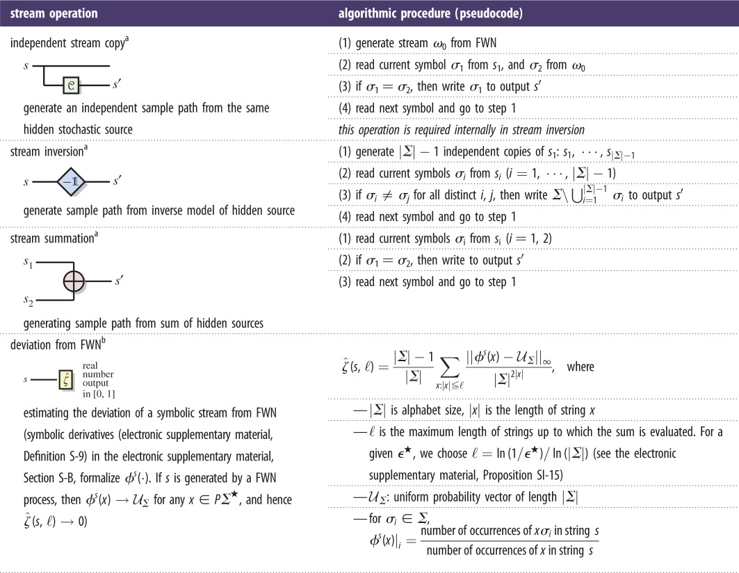^aSee the electronic supplementary material, Section S-F, for proof of correctness.

^bSee the electronic supplementary material, Definition S-22, Propositions S-14 and S-15 and Section S-F.

For any fixed alphabet size, the zero model is the unique single-state PFSA (up to minimal description [15]) that generates symbols as consecutive realizations of independent random variables with uniform distribution over the symbol alphabet. Thus, W generates FWN, and the entropy rate of FWN achieves the theoretical upper bound among the sequences generated by arbitrary PFSA in the model space. Two PFSAs G, H are identical if and only if G + (−H) = W.

3.2. Metric structure on model space

In addition to the Abelian group, the PFSA space admits a metric structure (see the electronic supplementary material, Section S-D). The distance between two models thus can be interpreted as the deviation of their group-theoretic difference from a FWN process. Data smashing exploits the possibility of estimating causal similarity between observed data streams by estimating this distance from the observed sequences alone without requiring the models themselves.

We can easily estimate the distance of the hidden model from FWN given only an observed stream s. This is achieved by the function (see table 1, row 4).

Intuitively, given an observed sequence fragment x, we first compute the deviation of the distribution of the next symbol from the uniform distribution over the alphabet. is the sum of these deviations for all historical fragments x with length up to ℓ, weighted by . The weighted sum ensures that deviation of the distributions for longer x have smaller contribution to , which addresses the issue that the occurrence frequencies of longer sequences are more variable.

4. Key insight: annihilation of information

Our key insight is the following: two sets of sequential observations have the same generative process if the inverted copy of one can annihilate the statistical information contained in the other. We claim that given two symbol streams s₁ and s₂, we can check whether the underlying PFSAs (say G₁, G₂) satisfy the annihilation equality G₁ + (−G₂) = W without explicitly knowing or constructing the models themselves.

Data smashing is predicated on being able to invert and sum streams, and to compare streams to noise. Inversion generates a stream s′ given a stream s, such that if PFSA G is the source for s, then −G is the source for s′. Summation collides two streams: given streams s₁ and s₂ generate a new stream s′ which is a realization of FWN if and only if the hidden models G₁, G₂ satisfy G₁ + G₂ = W. Finally, deviation of a stream s from that generated by a FWN process can be calculated directly.

Importantly, for a stream s (with generator G), the inverted stream s′ is not unique. Any symbol stream generated from the inverse model −G qualifies as an inverse for s; thus anti-streams are non-unique. What is indeed unique is the generating inverse PFSA model. As our technique compares the hidden stochastic processes and not their possibly non-unique realizations, the non-uniqueness of anti-streams is not problematic.

However, carrying out these operations in the absence of the model is problematic. In particular, we have no means to correct for any mis-synchronization of the states of the hidden models. Additionally, we want a linear-time algorithm, implying that it is desirable to carry out these operations in a memoryless symbol-by-symbol fashion. Thus, we use the notion of a pseudo-copies of probabilistic automata: given a PFSA G with a transition probability metric Π, a pseudo-copy (G) is any PFSA which has the same structure as G, but with a transition matrix

4.1

for some scalar . We show that the operations described above can be carried out efficiently, once we are willing to settle for stream realizations from pseudo-copies instead of the exact models. This does not cause a problem in disambiguation of hidden dynamics, because the invertibility of the map in equation (4.1) guarantees that pseudo-copies of distinct models remain distinct, and nearly identical hidden models produce nearly identical pseudo-copies.

Thus, despite the possibility of mis-synchronization between hidden model states, applicability of the algorithms shown in table 1 for disambiguation of hidden dynamics is valid. We show in the electronic supplementary material, Section S-F, that the algorithms evaluate distinct models to be distinct, and nearly identical hidden models to be nearly identical.

Estimating the deviation of a stream from FWN is straightforward (as specified by in table 1, row 4). All subsequences of a given length must necessarily occur with the same frequency for a FWN process; and we simply estimate the deviation from this behaviour in the observed sequence. The other two tasks are carried out via selective erasure of symbols from the input stream(s) (see table 1, rows 1–3). For example, summation of streams is realized as follows: given two streams s₁, s₂, we read a symbol from each stream, and if they match then we copy it to our output and ignore the symbols read when they do not match.

Thus, data smashing allows us to manipulate streams via selective erasure, to estimate a distance between the hidden stochastic sources. Specifically, we estimate the degree to which the sum of a stream and its anti-stream brings the entropy rate of the resultant stream close to its theoretical upper bound.

4.1. Contrast with feature-based state of art

Contemporary research in machine learning is dominated by the search for good ‘features' [16], which are typically understood to be heuristically chosen discriminative attributes characterizing objects or phenomena of interest. Finding such attributes is not easy [17,18]. Moreover, the number of characterizing features, i.e. the size of the feature set, needs to be relatively small to avoid intractability of the subsequent learning algorithms. Additionally, their heuristic definition precludes any notion of optimality; it is impossible to quantify the quality of a given feature set in any absolute terms; we can only compare how it performs in the context of a specific task against a few selected variations.

In addition to the heuristic nature of feature selection, machine learning algorithms typically necessitate the choice of a distance metric in the feature space. For example, the classic ‘nearest neighbour’ k-NN classifier [19] requires definition of proximity, and the k-means algorithm [20] depends on pairwise distances in the feature space for clustering. To side-step the heuristic metric problem, recent approaches often learn appropriate metrics directly from data, attempting to ‘back out’ a metric from side information or labelled constraints [21]. Unsupervised approaches use dimensionality reduction and embedding strategies to uncover the geometric structure of geodesics in the feature space (e.g. see manifold learning [22–24]). However, automatically inferred data geometry in the feature space is, again, strongly dependent on the initial choice of features. As Euclidean distances between feature vectors are often misleading [22], heuristic features make it impossible to conceive of a task-independent universal metric.

By contrast, smashing is based on an application-independent notion of similarity between quantized sample paths observed from hidden stochastic processes. Our universal metric quantifies the degree to which the summation of the inverted copy of any one stream to the other annihilates the existing statistical dependencies, leaving behind FWN. We circumvent the need for features altogether (see figure 1b) and do not require training.

Despite the fact that the estimation of similarities between two data streams is performed in the absence of the knowledge of the underlying source structure or its parameters, we establish that this universal metric is causal, i.e. with sufficient data it converges to a well-defined distance between the hidden stochastic sources themselves, without ever knowing them explicitly.

4.2. Contrast with existing model-free approaches to time-series analysis

Assumption-free time-series analysis to identify localized discords or anomalies has been studied extensively [6,7,25,26]. A significant majority of these reported approaches use SAX [10] for representing the possibly continuous-valued raw data streams. In contrast to our more naive quantization approach, where we map individual raw data streams to individual symbol sequences, SAX typically outputs a set of short symbol sequences (referred to as the SAX-words) obtained via quantization over a sliding window on a smoothed version of the raw data stream (see the electronic supplementary material, Section S-C, for a more detailed discussion). While the quantization details are somewhat different, both approaches essentially attempt to use information from the occurrence frequency of symbols or symbol-histories. However, choosing the length of the SAX-words beforehand amounts to knowing a priori the memory in the underlying process. By contrast, data smashing does not pre-assume any finite bound on the memory, and the self-annihilation error (see §5) provides us with a tool to check if the amount of available data is sufficient for carrying out the operations described in table 1. The underlying processes need to be at least approximately ergodic and stationary for both approaches. Nevertheless, data smashing is more advantageous for slow-mixing conditions, and for a fixed chosen word-length, the processes induce similar frequency of observed sequence fragments (see the electronic supplementary material, Section S-J). Importantly, no reported technique, to the best of our knowledge, has a built-in automatic check for data sufficiency that the self-annihilation error provides for data smashing.

SAX by itself does not lead to any notion of universal similarity. However, the NCM based on Kolmogorov complexity has been successfully used on symbolized data streams for parameter-free data mining and clustering [8]. While NCM is an elegant universal metric, the distance computed via smashing reflects similarity in a more intuitive manner; data from identical generators always mutually annihilate to FWN, implying that identical generators generate similar data streams (see the electronic supplementary material, Section S-I). Additionally, NCM needs to approximately ‘calculate’ incomputable quantities, and in theory needs to allow for unspecified additive constants. By contrast, we can compute the asymptotic convergence rate of the self-annihilation error.

5. Algorithmic steps

5.1. Self-annihilation test for data-sufficiency check

The statistical characteristics of the underlying processes, e.g. the correlation lengths, dictate the amount of data required for estimation of the proposed distance. With no access to the hidden models, we cannot estimate the required data length a priori; however, it is possible to check for data sufficiency for a specified error threshold via self-annihilation. As the proposed metric is causal, the distance between two independent samples from the same source always converges to zero. We estimate the degree of self-annihilation achieved in order to determine data sufficiency; that is, a stream is sufficiently long if it can sufficiently annihilate an inverted self-copy to FWN.

The self-annihilation-based data-sufficiency test consists of two steps: given an observed symbolic sequence s, we first generate an independent copy (say s′). This is the independent stream copy operation (see table 1, row 1), which can be carried out via selective symbol erasure without any knowledge of the source itself. Once we have s and s′, we check if the inverted version of one annihilates the other to a pre-specified degree. If a stream is not able to annihilate its inverted copy, it is too short for data smashing (see the electronic supplementary material, Section S-F).

Selective erasure in annihilation (see table 1) implies that the output tested for being FWN is shorter compared with the input stream, and the expected shortening ratio β can be explicitly computed (see the electronic supplementary material, Section S-F). We refer to β as the annihilation efficiency, because the convergence rate of the self-annihilation error scales asymptotically as (see the electronic supplementary material, Proposition S-16). In other words, the required length |s| of the data stream to achieve a self-annihilation error of scales as . Importantly, electronic supplementary material, Proposition S-13, shows that the annihilation efficiency is independent of the descriptional complexity, i.e. the number of causal states, in the underlying generating process. This, in combination with the electronic supplementary material, Proposition S-16, implies that the convergence of the self-annihilation error is asymptotically independent of the number of states in the process (see the electronic supplementary material, Section S-F, for detailed discussion following Proposition S-16). As an illustration, note that in the electronic supplementary material, figure S9, the self-annihilation error for a simpler two state process converges faster to a four state process. Note that the convergence rate is true only in an asymptotic sense, and the mixing time of the underlying process does indeed affect how fast the error drops with input length.

The self-annihilation error is also useful to rank the effectiveness of different quantization schemes. Better quantization schemes (e.g. ternary instead of binary) will be able to produce better self-annihilation while maintaining the ability to discriminate different streams (see the electronic supplementary material, Section S-C).

5.2. Feature-free classification and clustering

Given n data streams s₁, … , s_n, we construct a matrix E, such that E_ij represents the estimated distance between the streams s_i,s_j. Thus, the diagonal elements of E are the self-annihilation errors, while the off-diagonal elements represent inter-stream similarity estimates (see figure 2d for the basic annihilation circuit). This circuit yields three non-negative real numbers , which define the corresponding ijth entries of E. Given a positive threshold , the self-annihilation tests are passed if (k = i,j), and for sufficient data the streams s_i,s_j have identical sources with high probability if and only if . Once E is constructed, we can determine clusters by rearranging E into prominent diagonal blocks. Any standard technique [27] can be used for such clustering; data smashing is only used to find the causal distances between observed data streams, and the resultant distance matrix can then be used as input to state-of-the-art clustering methodologies or finding geometric structures (such as lower dimensional embedding manifolds [22]) induced by the similarity metric on the data sources.

The matrix H, obtained from E by setting the diagonal entries to zero, estimates a distance matrix. A Euclidean -embedding [28] of H then leads to deeper insight into the geometry of the space of the hidden generators. For example, in the case of the EEG data, the time series' embedding describe a one-dimensional manifold (a curve), with data from similar phenomena clustered together along the curve (see figure 3a(ii)).

5.3. Computational complexity

The asymptotic time complexity of carrying out the stream operations scales linearly with input length and the granularity of the alphabet (see the electronic supplementary material, Section S-F, and figure 4b for illustration of the linear-time complexity of estimating inter-stream similarity).

Figure 4.

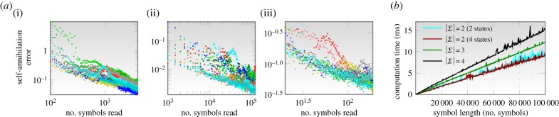
Computational complexity and convergence rates for data smashing. (a) Exponential convergence of the self-annihilation error for a small set of data series for different applications ((i) for EEG data, (ii) for heart sound recordings and (iii) for photometry). (b) Computation times for carrying out annihilation using the circuit shown in figure 2d as a function of the length of input streams for different alphabet sizes (and for different number of states in the hidden models). Note that the asymptotic time complexity of obtaining the similarity distances scales as , where n is the length of the shorter of the two input streams. (Online version in colour.)

6. Limitations and assumptions

Data smashing is not directly useful in problems which do not require a notion of similarity, e.g. predicting the future course of a time series, or for problems that do not involve the analysis of a stream, such as comparing images or unordered datasets.

For problems to which smashing is applicable, we implicitly assume the existence of PFSA generators, although we never find these models explicitly. It follows that what we actually assume is not any particular modelling framework, but that the systems of interest satisfy the properties of ergodicity, stationarity and have a finite (but not a priori bounded) number of states (see the electronic supplementary material, Section S-D). In practice, our technique performs well even if these properties are only approximately satisfied (e.g. quasi-stationarity instead of stationarity; see example in the electronic supplementary material, Section S-H). The algebraic structure of the space of PFSAs (in particular, existence of unique group inverses) is key to data smashing; however, we argue that any quantized ergodic stationary stochastic process is indeed representable as a probabilistic automata (see the electronic supplementary material, Section S-D).

Data smashing is not applicable to data from strictly deterministic systems. Such systems are representable by probabilistic automata; however, transitions occur with probabilities which are either 0 or 1. PFSAs with zero-probability transitions are non-invertible, which invalidates the underlying theoretical guarantees (see the electronic supplementary material, Section S-E). Similarly, data streams in which some alphabet symbol is exceedingly rare would be difficult to invert (see the electronic supplementary material, Section S-F, for the notion of annihilation efficiency).

Symbolization of a continuous data stream invariably introduces quantization error. This can be made small by using larger alphabets. However, larger alphabet sizes demand longer observed sequences (see the electronic supplementary material, Section S-F and figure S8), implying that the length of observation limits the quantization granularity, and in the process limits the degree to which the quantization error can be mitigated. Importantly, with coarse quantizations distinct processes may evaluate to be similar. However, identical processes will still evaluate to be identical (or nearly so), provided the streams pass the self-annihilation test. The self-annihilation test thus offers an application-independent way to compare and rank quantization schemes (see the electronic supplementary material, Section S-C).

The algorithmic steps (see table 1) require no synchronization (we can start reading the streams anywhere), implying that non-equal length of time series, and phase mismatches are of no consequence.

7. Application examples

Data smashing begins with quantizing streams to symbolic sequences, followed by the use of the annihilation circuit (figure 2d) to compute pairwise causal similarities. Details of the quantization schemes, computed distance matrices and identified clusters and Euclidean embeddings are summarized in table 2 and figure 3 (see also the electronic supplementary material, Sections S-A and S-C).

Table 2.

Application problems and results (see the electronic supplementary material, table S1, for a more detailed version).

system	input description	classification performance
(1) identify epileptic pathology [29]	— 495 EEG excerpts, each 23.6 s sampled at 173.61 Hz — signal derivative as input — quantizationa (three letter):	no comparable result is available in the literature. However, IA reveals a one-dimensional manifold structure in the dataset, while [29] with additional assumptions on the nature of hidden processes fails to yield such insight
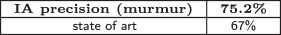
(2) identify heart murmur [30]	— 65 .wav files sampled at 44.1 kHz (approx. 10 s each) — quantizationa (two letter):	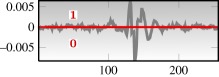state of the art [30] achieved in supervised learning with task-specific features
(3) classify variable stars (Cepheid variable versus RR Lyrae) from photometry (OGLE II) [31]	— 10 699 photometric series — differentiated folded/raw photometry used as input — quantizationa (three letter):	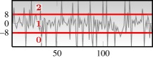state of the art [31] achieved with task-specific features and multiple hand-optimized classification steps 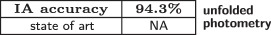(this capability is beyond the state of art)
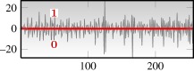
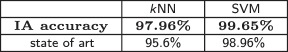
(4) EEG-based biometric authentication [32] with visually evoked potentials	— 122 subjects, multi-variate data from 61 standard electrodes — 256 data points for each trial for each electrode — total number of data series: 5477 (each with 61 variables) — quantizationa (two letter):	state of the art [33] achieved with task-specific features, and after eliminating two subjects from consideration
(5) text-independent speaker identification using ELSDSR database [34]	— 23 speakers (9 female, 14 male), 16 kHz recording — approximately 100 s recording/speaker — 2 s snippets used as time-series excerpts — total number of time series: 1270 — quantizationa (two letter):	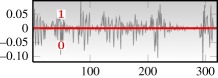state of the art [35] achieved with task-specific features and multiple hand-optimized classification steps

^aSee the electronic supplementary material, Section S-C, for details on choosing quantization schemes.

Our first application is classification of brain electrical activity from different physiological and pathological brain states [29]. We used sets of EEG data series consisting of surface EEG recordings from healthy volunteers with eyes closed and open, and intracranial recordings from epilepsy patients during seizure-free intervals from within and from outside the seizure generating area, as well as intracranial recordings of seizures.

Starting with the data series of electric potentials, we generated sequences of relative changes between consecutive values before quantization. This step allows a common alphabet for sequences with wide variability in the sequence mean values.

The distance matrix from pairwise smashing yielded clear clusters corresponding to seizure, normal eyes open, normal eyes closed and epileptic pathology in non-seizure conditions (see figure 3a, seizures not shown due to large differences from the rest).

Embedding the distance matrix (see figure 3a(i)) yields a one-dimensional manifold (a curve), with contiguous segments corresponding to different brain states, e.g. right-hand side of plane A corresponds to epileptic pathology. This provides a particularly insightful picture, which eludes complex nonlinear modelling [29].

Next, we classify cardiac rhythms from noisy heat–sound data recorded using a digital stethoscope [30]. We analysed 65 data series (ignoring the labels) corresponding to healthy rhythms and murmur, to verify if we could identify clusters without supervision that correspond to the expert-assigned labels.

We found 11 clusters in the distance matrix (see figure 3b), four of which consisted of mainly data with murmur (as determined by the expert labels), and the rest consisting of mainly healthy rhythms (see figure 3b(iv)). Classification precision for murmur is noted in table 2 (75.2%). Embedding of the distance matrix revealed a two-dimensional manifold (see figure 3b(iii)).

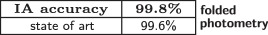
Our next problem is the classification of variable stars using light intensity series (photometry) from the optical gravitational lensing experiment (OGLE) survey [31]. Supervised classification of photometry proceeds by first ‘folding’ each light-curve to its known period to correct phase mismatches. In our first analysis, we started with folded light-curves and generated data series of the relative changes between consecutive brightness values in the curves before quantization, which allows for the use of a common alphabet for light-curves with wide variability in the mean brightness values. Using data for Cepheids and RR Lyrae (3426 Cepheids, 7273 RR Lyrae), we obtained a classification accuracy of 99.8% which marginally outperforms the state of art (see table 2). Clear clusters (obtained unsupervised) corresponding to the two classes can be seen in the computed distance matrix (see figure 3c(i)) and the three-dimensional projection of its Euclidean embedding (see figure 3c(ii)). The three-dimensional embedding was very nearly constrained within a two-dimensional manifold (see figure 3c(ii)).

Additionally, in our second analysis, we asked if data smashing can work without knowledge of the period of the variable star; skipping the folding step. Smashing raw photometry data yielded a classification accuracy of 94.3% for the two classes (see table 2). This direct approach is beyond state of the art techniques.

Our fourth application is biometric authentication using visually evoked EEG potentials. The public database used [32] considered 122 subjects, each of whom was exposed to pictures of objects chosen from the standardized Snodgrass set [36].

Note that while this application is supervised (as we are not attempting to find clusters unsupervised), no actual training is involved; we merely mark the randomly chosen subject-specific set of data series as the library set representing each individual subject. If ‘unknown’ test data series is smashed against each element of each of the libraries corresponding to the individual subjects, we expected that the data series from the same subject will annihilate each other correctly, whereas those from different subjects will fail to do so to the same extent. We outperformed the state of art for both kNN- and SVM-based approaches (see table 2, and the electronic supplementary material, Section S-A).

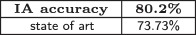
Our fifth application is text-independent speaker identification using the ELSDSR database [34], which includes recording from 23 speakers (9 female and 14 male, with possibly non-native accents). As before, training involved specifying the library series for each speaker. We computed the distance matrix by smashing the library data series against each other and trained a simple kNN on the Euclidean embedding of the distance matrix. The test data then yielded a classification accuracy of 80.2%, which beat the state of art figure of 73.73% for 2 s snippets of recording data [35] (see table 2 and the electronic supplementary material, figure S1b).

8. Conclusion

We introduced data smashing to measure causal similarity between series of sequential observations. We demonstrated that our insight allows feature-less model-free classification in diverse applications, without the need for training, or expert tuned heuristics. Non-equal length of time series, missing data and possible phase mismatches are of little consequence.

While better classification algorithms likely exist for specific problem domains, such algorithms are difficult to develop and tune. The strength of data smashing lies in its ability to circumvent both the need for expert-defined heuristic features and expensive training, thereby eliminating one of the major bottlenecks in contemporary big data challenges.

Funding statement

This work has been supported in part by US Defense Advanced Research Projects Agency (DARPA) project W911NF-12-1-0449, and the US Army Research Office (ARO) project W911NF-12-1-0499.

References

- 1.Cover TM, Thomas JA. 1991. Elements of information theory. New York, NY: John Wiley. [Google Scholar]
- 2.Duin RPW, de Ridder D, Tax DMJ. 1997. Experiments with a feature-less approach to pattern recognition. Pattern Recognit. Lett. 18, 1159–1166. ( 10.1016/S0167-8655(97)00138-4) [DOI] [Google Scholar]
- 3.Mottl V, Dvoenko S, Seredin O, Kulikowski C, Muchnik J. 2001. Featureless pattern recognition in an imaginary Hilbert space and its application to protein fold classification. In Machine learning and data mining in pattern recognition (ed. P Perner). Lecture Notes in Computer Science, vol. 2123, pp. 322–336. Berlin, Germany: Springer. ( 10.1007/3-540-44596-X_26) [DOI] [Google Scholar]
- 4.Pekalska E, Duin RPW. 2002. Dissimilarity representations allow for building good classifiers. Pattern Recognit. Lett. 23, 943–956. ( 10.1016/S0167-8655(02)00024-7) [DOI] [Google Scholar]
- 5.Li M, Chen X, Li X, Ma B, Vitanyi PMB. 2004. The similarity metric. IEEE Trans. Inform. Theory 50, 3250–3264. ( 10.1109/TIT.2004.838101) [DOI] [Google Scholar]
- 6.Ratanamahatana C, Keogh E, Bagnall AJ, Lonardi S. 2005. A novel bit level time series representation with implication of similarity search and clustering. In Advances in knowledge discovery and data mining (eds Ho T, Cheung D, Liu H.). Lecture Notes in Computer Science, vol. 3518, pp. 771–777 Berlin, Germany: Springer; ( 10.1007/11430919_90) [DOI] [Google Scholar]
- 7.Wei L, Kumar N, Lolla V, Keogh EJ, Lonardi S, Ratanamahatana C. 2005. Assumption-free anomaly detection in time series. In Proc. 17th Int. Conf. on Scientific and Statistical Database Management, pp. 237–240. Berkeley, CA: Lawrence Berkeley Laboratory. [Google Scholar]
- 8.Keogh E, Lonardi S, Ratanamahatana CA. 2004. Towards parameter-free data mining. In Proc. 10th ACM SIGKDD Int. Conf. on Knowledge Discovery and Data Mining, pp. 206–215. New York, NY: ACM. ( 10.1145/1014052.1014077) [DOI] [Google Scholar]
- 9.Anthony B, Ratanamahatana C, Keogh E, Lonardi S, Janacek G. 2006. A bit level representation for time series data mining with shape based similarity. Data Min. Knowl. Discov. 13, 11–40. ( 10.1007/s10618-005-0028-0) [DOI] [Google Scholar]
- 10.Keogh E, Lin J, Fu A. 2005. HOT SAX: efficiently finding the most unusual time series subsequence. In Proc. 5th IEEE Int. Conf. on Data Mining, pp. 226–233. Washington, DC: IEEE Computer Society; ( 10.1109/ICDM.2005.79) [DOI] [Google Scholar]
- 11.Chattopadhyay I, Lipson H. 2013. Abductive learning of quantized stochastic processes with probabilistic finite automata. Phil. Trans. R. Soc. A 371, 20110543 ( 10.1098/rsta.2011.0543) [DOI] [PubMed] [Google Scholar]
- 12.Crutchfield JP, McNamara BS. 1987. Equations of motion from a data series. Complex Syst. 1, 417–452. [Google Scholar]
- 13.Crutchfield JP. 1994. The calculi of emergence: computation, dynamics and induction. Phys. D Nonlinear Phenom. 75, 11–54. ( 10.1016/0167-2789(94)90273-9) [DOI] [Google Scholar]
- 14.Chattopadhyay I, Wen Y, Ray A. 2010. Pattern classification in symbolic streams via semantic annihilation of information. (http://arxiv.org/abs/1008.3667) [Google Scholar]
- 15.Chattopadhyay I, Ray A. 2008. Structural transformations of probabilistic finite state machines. Int. J. Control 81, 820–835. ( 10.1080/00207170701704746) [DOI] [Google Scholar]
- 16.Duda RO, Hart PE, Stork DG. 2000. Pattern classification, 2nd edn New York, NY: Wiley-Interscience. [Google Scholar]
- 17.Brumfiel G. 2011. High-energy physics: down the petabyte highway. Nature 469, 282–283. ( 10.1038/469282a) [DOI] [PubMed] [Google Scholar]
- 18.Baraniuk RG. 2011. More is less: signal processing and the data deluge. Science 331, 717–719. ( 10.1126/science.1197448) [DOI] [PubMed] [Google Scholar]
- 19.Cover T, Hart P. 1967. Nearest neighbor pattern classification. IEEE Trans. Inform. Theory 13, 21–27. ( 10.1109/TIT.1967.1053964) [DOI] [Google Scholar]
- 20.MacQueen JB. 1967. Some methods for classification and analysis of multivariate observations. In Proc. 5th Berkeley Symp. on Mathematical Statistics and Probability, pp. 281–297. Berkeley, CA: University of California Press. [Google Scholar]
- 21.Yang L. 2007. An overview of distance metric learning. In Proc. Computer Vision and Pattern recognition, 7 October. [Google Scholar]
- 22.Tenenbaum J, de Silva V, Langford J. 2000. A global geometric framework for nonlinear dimensionality reduction. Science 290, 2319–2323. ( 10.1126/science.290.5500.2319) [DOI] [PubMed] [Google Scholar]
- 23.Roweis S, Saul L. 2000. Nonlinear dimensionality reduction by locally linear embedding. Science 2900, 2323–2326. ( 10.1126/science.290.5500.2323) [DOI] [PubMed] [Google Scholar]
- 24.Seung H, Lee D. 2000. Cognition. The manifold ways of perception. Science 290, 2268–2269. ( 10.1126/science.290.5500.2268) [DOI] [PubMed] [Google Scholar]
- 25.Kumar N, Lolla N, Keogh E, Lonardi S, Ratanamahatana CA. 2005. Time-series bitmaps: a practical visualization tool for working with large time series databases. In Proc. SIAM 2005 Data Mining Conf. (ed. Kargupta H, et al.), pp. 531–535. Philadelphia, PA: SIAM. [Google Scholar]
- 26.Wei L, Keogh E, Xi X, Lonardi S. 2005. Integrating lite-weight but ubiquitous data mining into GUI operating systems. J. Univers. Comput. Sci. 11, 1820–1834. [Google Scholar]
- 27.Ward JH. 1963. Hierarchical grouping to optimize an objective function. J. Am. Stat. Assoc. 58, 236–244. ( 10.1080/01621459.1963.10500845) [DOI] [Google Scholar]
- 28.Sippl MJ, Scheraga HA. 1985. Solution of the embedding problem and decomposition of symmetric matrices. Proc. Natl Acad. Sci. USA 82, 2197–2201. ( 10.1073/pnas.82.8.2197) [DOI] [PMC free article] [PubMed] [Google Scholar]
- 29.Andrzejak RG, Lehnertz K, Mormann F, Rieke C, David P, Elger CE. 2001. Indications of nonlinear deterministic and finite dimensional structures in time series of brain electrical activity: dependence on recording region and brain state. Phys. Rev. E 64, 061907 ( 10.1103/PhysRevE.64.061907) [DOI] [PubMed] [Google Scholar]
- 30.Bentley P, et al. 2011. The PASCAL Classifying Heart Sounds Challenge 2011 (CHSC2011) Results See http://www.peterjbentley.com/heartchallenge/index.html.
- 31.Szymanski MK. 2005. The optical gravitational lensing experiment. Internet access to the OGLE photometry data set: OGLE-II BVI maps and I-band data. Acta Astron. 55, 43–57. [Google Scholar]
- 32.Begleiter H. 1995. EEG database data set. New York, NY: Neurodynamics Laboratory, State University of New York Health Center Brooklyn; See http://archive.ics.uci.edu/ml/datasets/EEG+Database. [Google Scholar]
- 33.Brigham K, Kumar BVKV. 2010. Subject identification from electroencephalogram (EEG) signals during imagined speech. In 4th IEEE Int. Conf. on Biometrics: Theory Applications and Systems ( BTAS ), pp. 1–8, ( 10.1109/BTAS.2010.5634515) [DOI] [Google Scholar]
- 34.English Language Speech Database for Speaker Recognition. Department of Informatics and Mathematical Modelling, Technical University of Denmark. 2005 See http://www2.imm.dtu.dk/~lfen/elsdsr/.
- 35.Feng L, Hansen LK. 2005. A new database for speaker recognition. IMM technical report 2005-05. Kgs. Lyngby, Denmark: Technical University of Denmark, DTU See http://www2.imm.dtu.dk/pubdb/p.php?3662. [Google Scholar]
- 36.Snodgrass JG, Vanderwart M. 1980. A standardized set of 260 pictures: norms for name agreement, image agreement, familiarity, and visual complexity. J. Exp. Psychol. Hum. Learn. Mem. 6, 174–215. ( 10.1037/0278-7393.6.2.174) [DOI] [PubMed] [Google Scholar]
Associated Data
This section collects any data citations, data availability statements, or supplementary materials included in this article.