Universals versus historical contingencies in lexical evolution

Abstract

The frequency with which we use different words changes all the time, and every so often, a new lexical item is invented or another one ceases to be used. Beyond a small sample of lexical items whose properties are well studied, little is known about the dynamics of lexical evolution. How do the lexical inventories of languages, viewed as entire systems, evolve? Is the rate of evolution of the lexicon contingent upon historical factors or is it driven by regularities, perhaps to do with universals of cognition and social interaction? We address these questions using the Google Books N-Gram Corpus as a source of data and relative entropy as a measure of changes in the frequency distributions of words. It turns out that there are both universals and historical contingencies at work. Across several languages, we observe similar rates of change, but only at timescales of at least around five decades. At shorter timescales, the rate of change is highly variable and differs between languages. Major societal transformations as well as catastrophic events such as wars lead to increased change in frequency distributions, whereas stability in society has a dampening effect on lexical evolution.

1. Introduction

In linguistics, discussions of rates of lexical change have revolved around the idea, introduced by Morris Swadesh, that a small core of the vocabulary, which has come to be known as ‘the Swadesh list’, has a characteristic degree of stability, making it possible to date the diversification of groups of related languages by observing the amount of change within such a list of basic vocabulary [1,2]. This so-called glottochronological method has had the curious fate of having been criticized to the extent that it is often routinely dismissed as being ‘discredited’ [3–5] whereas, at the same time, glottochronological dates are frequently cited, even by the critics of glottochronology [6], and many refinements of the method have been proposed, some [7] having had a great deal of impact. For many linguists, the fatal wounds inflicted upon glottochronology came from studies where some languages were shown to have had quite different rates of change [8]. But, such studies raise the question of whether the rate of change might still be sufficiently constant that it is useful for dating language group divergence with reasonable accuracy provided that averages over several languages are used and the time spans measured are great enough. A recent study from the project known as the Automated Similarity Judgment Program (ASJP) [9] uses a measure of phonological distance between words as another way of deriving dates of language group divergence. Glottochronology uses a count of cognates (related words) as its input. In this approach, word pairs will score 1 for being related and 0 for being unrelated. In the ASJP approach, unrelated words will usually have a similarity close to 0 and related words some number between 0 and 1. Thus, the ASJP approach is also sensitive to cognacy and therefore comparable to glottochronology. It was found in reference [9] that for 52 groups of languages whose divergence dates are approximately known, there is a –0.84 correlation between log similarity and time. Thus, the assumption of glottochronology of an approximately regular rate of change is vindicated in this study, which is the first to provide a test across many language groups.

Studies in glottochronology have been limited to short word lists, the maximum being a standard set of 200 items. The differential stabilities within the more popular 100-item Swadesh list have been measured [10], and the above-mentioned ASJP study [9] was conducted on a 40-item subset of the 100-item list. Beyond these short lists, little is known in quantitative terms about the dynamics of lexical change, and even within the 100-item list, the factors that contribute to making some items more or less stable than others are not well understood. The possibility that some items are less stable because they tend to be borrowed more often was investigated [10], but no correlation was found between borrowability and stability. However, stability and frequency have been found to be correlated [11], indicating that words that are used often tend to survive better than infrequently used words. These findings were based on the behaviour of a short (200 items) set of words. Similarly, it has been found that irregular morphological forms tend to survive longer in their irregular forms without being regularized the more frequent they are [12].

The availability of the large Google Books Corpus (https://books.google.com/ngrams/) has dramatically increased the amount of data available for studying lexical dynamics, allowing us to look at thousands of different words. But, the time span of half a millennium for which printed books are available is not great enough to study the replacement rates of all lexical items—it is only in some cases that we can observe one item being entirely replaced by another, and if a word survives for 500 years, we cannot know what its likely longevity is beyond the 500 years. Moreover, eight languages, which is what the Google Books Corpus offers, is not enough to establish whether words associated with particular meanings are more or less prone to change across languages.

We can nevertheless still indirectly investigate to what degree the rate of lexical change is constant in words not pertaining to the Swadesh list. The Google Books N-Gram Corpus allows us to study changing frequency distributions of entire word inventories year by year over hundreds of years. Inasmuch as the gain or loss of a lexical item presupposes a change in its frequency, there is a relationship, possibly one of proportionality, between frequency changes and gain/loss. In other words, it is meaningful to use frequency change as a proxy for lexical change in general. By ‘lexical change’, we refer mainly to processes whereby one form covering a certain meaning is gradually being replaced by another because of a change in the semantic scope of the original lexical item and/or because of the innovation of new words.

In this paper, we address the question of the constancy of the rate of lexical change beyond the Swadesh list by studying changes in frequency distributions. In so doing, we will observe that the rate of change over short time intervals is anything but constant, leading to additional questions about which factors might cause this variability. Comparisons of British and American English will hint at processes by which innovations arise and spread; observations of changing frequency distributions over time will disclose effects of historical events and comparisons across languages will help us to discern some universal tendencies cutting across effects of historical contingencies. It should of course be kept in mind that the data consist of written, mostly literary, language. Written language tends to be more conservative than spoken language, so changes observed are likely to be more enhanced in the spoken language.

This is not the first paper to draw on the Google Books N-Gram Corpus. Since the seminal publication introducing this resource as well as the new concept of ‘culturomics' [13], papers have been published that have analysed patterns of evolution of the usage of different words from a variety of perspectives, such as random fractal theory [14], Zipf's and Heaps' laws and their generalization to two-scaling regimes [15], the evolution of self-organization of word frequencies over time in written English [16], statistical properties of word growth [17,18], socio-historical determinants of word length dynamics [19]; and other studies have been more specifically aimed at issues such as the sociology of changing values resulting from urbanization [20] or changing concepts of happiness [21].

2. Materials

The Google Books N-Gram Corpus offers data on word frequencies from 1520 onwards based on a corpus of 862 billion words in eight languages. Of these, we will draw upon English, Russian, German, French, Spanish and Italian with particular attention to English, which conveniently is presented both as a total corpus (‘common English’) and also as subcorpora (British, American, fictional). Chinese and Hebrew are not included in the study, because the corpora available for these languages are relatively small. We focus on 1-grams, i.e. single words, and these are filtered such that only words containing letters of the basic alphabet of the relevant language plus a single apostrophe are admitted. Among other things, this excludes numbers. We furthermore ignored capitalization. For each language (or variety of a language in the case of English), the basic data consist of a year, the words occurring that year and their raw frequencies.

The version of the Google Books N-Gram Corpus used here is the second version, from 2012, but all analyses were in fact also carried out using the 2009 version. The second version, apart from being larger and including an extra language (Italian), mainly differs by the introduction of parts-of-speech (POS) tags [22]. The POS tags are inaccurate to the extent that for the great majority of words there are at least some tokens that are misclassified. For instance, some tokens of the word ‘internet’ are tagged as belonging to the categories adpositions, adverbs, determiners, numerals, pronouns, particle and ‘other’—all categories where ‘internet’ clearly cannot belong given that the word is a noun. In each of these clear cases of misclassification, it is only a small amount of tokens that are wrongly assigned, however. In the case of ‘internet’, the tokens that are put in each of the wrong categories make up from 0.004% (‘internet’ as an adverb) to 0.107% (‘internet’ as a verb). As many as 94.044% of the tokens are correctly classified as nouns. Finally, 5.443% of the tokens are put in the adjective category. This assignment is not obviously wrong, because ‘internet’ in a construction such as ‘internet café’ does share a characteristic with adjectives, namely that of modifying a noun. After manual inspection of the 300 most common English words, we came to the conclusion that a reasonable strategy for filtering out obviously wrong assignments would be to ignore cases where a POS tag is assigned to 1% or less of the total number of tokens of a given word.

In electronic supplementary material, figure S1, we replicate one of our results (see figure 1 of the Results section) on three different versions of the database: the 2009 version, the 2012 version ignoring POS tags altogether and the 2012 version including POS tags (but filtered as just described). There are some differences in behaviour for the 2009 version as opposed to the 2012 version with and without POS, especially in recent years. But, as it turns out, it would be possible to ignore POS tags altogether and not get appreciably different results for the 2012 version of the database. Nevertheless, they are included here.

Thus, when we speak of a ‘word’ or 1-gram in this paper, we are referring to any unique combination of a word form (whether distinct for morphological or purely lexical reasons) and a POS tag. Unless otherwise noted, all results were based on the 100 000 most frequent words in order to filter out most of the noise caused by errors of optical character recognition.

3. Methods

The sets of word frequencies for each year in a given language can be considered vectors, where changes in word usage affect the value of the vector components. The frequency of a word at a given time is here interpreted as the probability of its occurrence in the corpus pertaining to a given year. To estimate changes in the lexical profile, a metric is needed for determining distances between the vectors. In other words, given two probability (frequency) distributions, p_i^A and p_i^B, we need a suitable index for measuring the difference between them.

A frequently used class of metrics is shown in equation (3.1). For n = 1, it gives Manhattan distances, and for n = 2, it gives Euclidean distances

3.1

An information-theoretic metric, however, is expected to be more meaningful in our case, and the selection of such a metric is furthermore justified empirically in §4. First, in order to measure information, we use the standard formula in (3.2).

3.2

In order to calculate distances, we then apply the Kullback–Leibler (KL) metric [23] (equation (3.3)). Being asymmetric, this is not a true metric in the technical sense, but it can be symmetrized, as in equation (3.4)

3.3

3.4

The K–L divergence is commonly used in studies related to ours [24,25]. Being a measure of relative entropy, it measures the divergence of two frequency distributions with regard to their informational content. The informational content of a single occurrence of a word is proportional to the logarithm of its probability taken with the opposite sign. Thus, for a rare word and a commonly occurring word, one and the same change in frequency values has different implications for the change in entropy. Information is usually measured in bits, which accounts for why the logarithms are to base 2 in equations (3.2)–(3.4).

Because one cannot take the logarithm of zero, the situation where the frequency of a word in B is zero must be handled in a special way. A possible approach, which was tested, is to simply remove the ‘zero-cases' from the distribution. However, we handled the situation in a more principled way by replacing zero-frequencies by imputed frequencies based on the corresponding words in A as shown in the electronic supplementary material. In practice, however, no appreciable differences were observed in the results when applying the simpler as opposed to the more complicated approach.

The change in entropy D_A,B is normalized by the entropy of the changed frequency distribution (equation (3.5)). For the symmetrized version, we normalize by the sum of the two entropies (equation (3.6)).

3.5

3.6

When comparing frequency distributions at different time periods for one and the same language, we use the asymmetric K–L divergence (equations (3.3) and (3.5)). This was used to produce figures 1 and 7–9. When frequency distributions in different languages are compared, we use the symmetrized version (equations (3.4) and (3.6)). This was used to produce figures 2 and 3. When the unit of analysis is the frequency of individual words, neither is used (figures 4–6).

Figure 1.

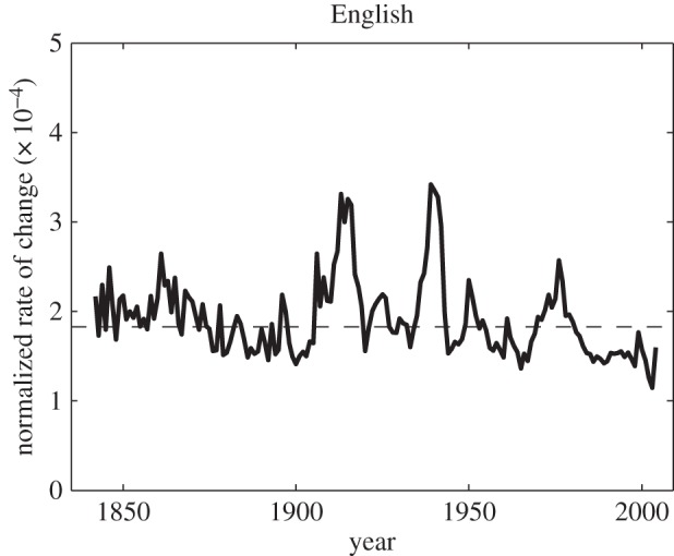
Change rates over time in the English lexicon.

Figure 7.

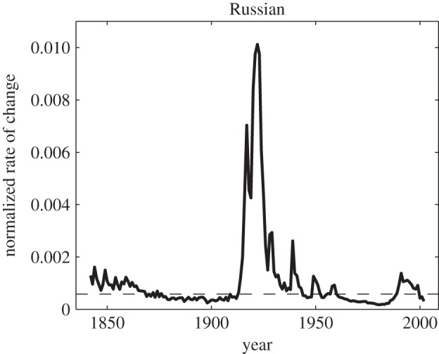
Change rates over time in the Russian lexicon.

Figure 9.

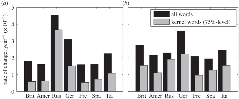
Rates of change in seven languages over (a) 10-year versus (b) 50-year intervals.

Figure 2.

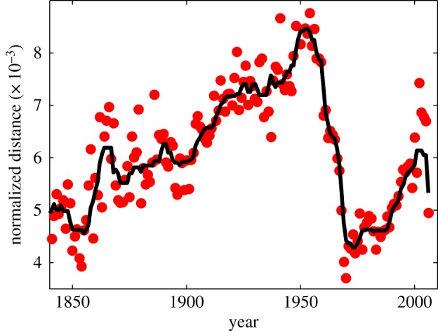
Distances between British and American English.

Figure 3.

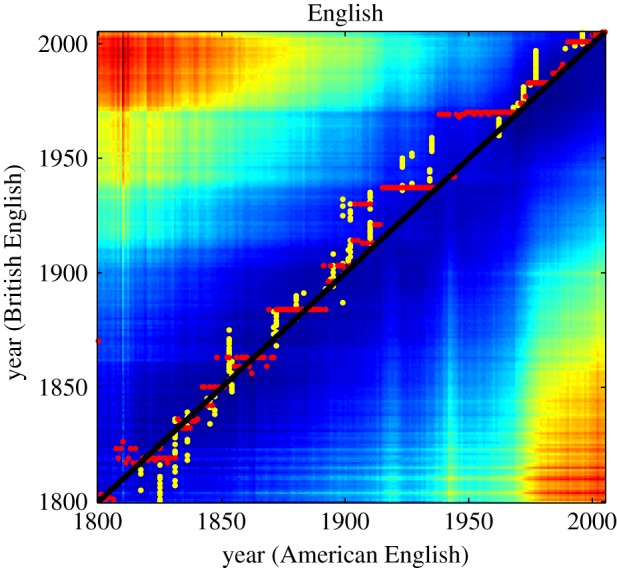
Distances between British and American English for any pair of years (1800–2008). The colour spectrum ranges from blue (=small distances) to red (=large distances). Yellow and red dots show local minimal distances. The diagonal is marked in black.

Figure 4.

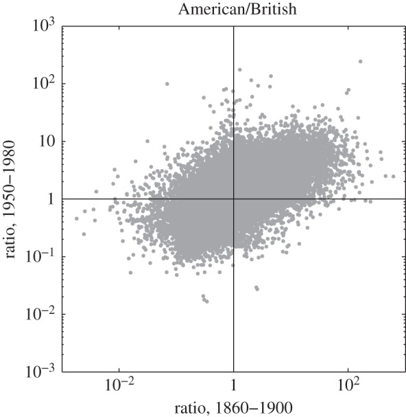
The ratio of Americanisms to Briticisms.

Figure 6.

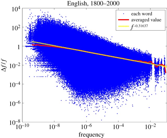
Relative frequency changes for English during 1800–2000 as a function of frequency. Average relative frequency changes (red line) are fitted to a power law (yellow dotted line).

We will sometimes refer to the ‘lexical rate of change’. This is defined as the average normalized K–L divergence per year between two points in time, t and t + T, as expressed in equation (3.7)

3.7

4. Results

We first look at changes in frequency distributions in the common English corpus, focusing on the period from 1840 onwards, when the amount of available books in good-quality printing is suitable.

Figure 1 shows a graph of normalized K–L distances between neighbouring states of the language year by year using a 10-year moving window, applying formula (3.7). A 10-year moving window means that T = 5. The mean of the normalized distances, taken across the per-year changes (calculated as explained in the previous sentence), is 〈V〉 = 1.93 × 10⁻⁴, the standard deviation s.d.(V) = 2.77 × 10⁻⁵, and s.d.(V)/(V) = 14.3%.

The graph shows some peaks corresponding to changes in lexical profile that clearly must be due to major political events, in addition to smaller, chaotic oscillations. Above all, peaks corresponding to the periods of each of the world wars catch the eye. Growth-rate fluctuations in the English lexicon have similarly been observed to be sensitive to these events [17]. The turbulent twentieth century stands in contrast to the period preceding it, where the fluctuations are generally smaller. This is the Victorian era, which was generally a stable period for British society. Thus, the presence of frequency changes can be provoked by major international historical events and, reversely, the potential for change is dampened by political stability. Over the approximately 150 year period that we are witnessing, these effects roughly cancel out.

Graphs based on the same data as in figure 1 were produced using the symmetrized version of K–L divergence (equation (3.4)) as well as Manhattan and Euclidean distances (equation (3.1)) for different values of n. For these graphs, see the electronic supplementary material, figures S2 and S3. For the symmetrized K–L divergence, the results are not appreciably different from figure 1; for Manhattan distances, we see a similar picture but with some dampening in the major peaks and for Euclidean distances, the effects of minor variation are enhanced to the extent that the effects of the two world wars become difficult to distinguish from fluctuations that are not obviously connected to historical events. This is the empirical motivation for our choice of K–L divergence as a preferred metric. The differences are most likely owing to Manhattan distances and K–L divergence being more sensitive than Euclidean distances to small, absolute changes in frequency, which mainly occur for rare words. These speculations are supported by figures 5 and 6, which show that more infrequent words suffer the greater frequency changes.

Figure 5.

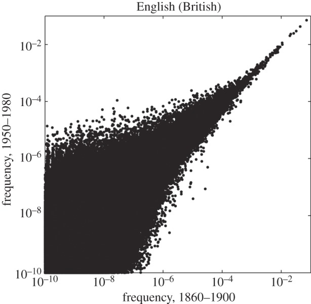
Average frequency of each lexical item during 1950–1980 as a function of its average frequency during 1860–1900.

Because the Google Books N-Gram Corpus distinguishes between British and American English, it is possible to study differences between the evolution of these two language variants as well as their interrelatedness. The lexicons of the two variants are practically identical in spite of differences in frequencies of items, so we can again use K–L divergence as a metric for comparing them. In figure 2, the dots show normalized distances for each year within the period 1840–2008, and the line shows the result of smoothing using a median filter with a 10-year window.

The two variants of English start out diverging more and more up to around 1950–1955, after which time they rapidly begin to converge; and from around 1975 onwards, they appear to fluctuate around the same level of divergence that they exhibited in 1840. No doubt the introduction of mass media has played a major role in this convergence.

Next, we may ask whether the two variants behave in a similar way. For instance, do they mutually converge towards one another at the same speed or is one of them converging faster? To answer this question, figure 3 shows a heat map where colours represent informational distances between any two points in time for the two variants, using the same data as for figure 2. Figure 3 (also provided in a more detailed three-dimensional version in figure S4 of the electronic supplementary material) reveals that between around 1900 and 2000 the smallest distances tend to lie above the diagonal rather than being scattered around it as before 1900. For instance, the American English data of 1920 are most similar to the British English data of around 1940. In general, for each year throughout the twentieth century, British English is conservative relative to American English, being most similar to American English of one to two decades earlier. This situation seems to change by the end of the century, although we are not yet far enough into the twenty-first century to be able to determine whether the convergence is a lasting trend. Were we to try to predict the future, however, our bet would be that British English will cease to be conservative relative to American English.

Additional information about the differences between British and American English is presented in figure 4, where words are classified as ‘Briticisms’ versus ‘Americanisms' for the two periods 1860–1900 and 1950–1980. A Briticism is defined as any word that is more frequent in British English than in American English in a given period, and an Americanism has the opposite definition. The specific periods were chosen for being around a century apart and relatively ‘quiet’ in the sense that they are not affected by any of the two major peaks in changes of frequency distributions that happened during the world wars. A four-way classification is produced by finding the ratio between American and British English of the frequencies of individual words. For instance, a ratio of r = 50 means that the frequency in American English is 50 times higher.

In the lower left are Briticisms that have stayed as such during both periods (35.5% of the total sample); in the upper right are Americanisms that have stayed as such during both periods (32.1%); in the lower right are Americanisms that have become Briticisms (16.0%); in the upper left are Briticisms that have become Americanisms (16.4%). There are somewhat more words that change from being Briticisms to Americanisms than the other way around, but the difference is small, and there are more words that remain as Briticisms than words that remain as Americanisms.

Having treated changes in English from the points of view of contingencies of history and particulars relating to the interaction between the major, British and American, variants, we now pass on to a question relating more to the universals of language change: which words are most sensitive to changes in frequency distributions? This question is investigated through two plots. First, in figure 5, we average frequencies for each item within the respective periods 1860–1900 and 1950–1980 and plot the latter as a function of the former. The boundaries for the time intervals were selected such that sample sizes are approximately equal: the total corpus size for 1860–1900 is 1.59×10¹⁰ words, and for 1950–1980, it is 1.65×10¹⁰ words thus, the difference is smaller than 4%.

Unlike the other figures, figure 5 is based on all words, not just the 100 000 most frequent ones. It shows, first of all, a wider range of variation in changes in frequency distributions as frequencies decrease. Words with a frequency of around 10^–3 or higher do not change their frequency radically, leading to dots gathered narrowly around a straight line. These include function words—articles, prepositions and conjunctions. For words which have frequencies in the less than 10⁻³ range, the distribution widens symmetrically, indicating that these words may either increase or decrease their frequencies, and that the relative changes of frequency values grow with decreasing frequencies.

The impression of figure 5 that the range of frequency changes increases as frequency decreases is brought out more clearly by figure 6, which is also based on all words rather than the 100 000 most frequent ones. The horizontal axis shows the frequency f, and the vertical axis shows the relative frequency change Δf/f of words for a 1-year period. The blue dots show the values of Δf/f for the individual words in a given year. There are 6 783 304 different words in the corpus for the 200-year period, so the number of dots could theoretically be 6 783 304×200, but because not every word is attested in every pair of consecutive years, the number of dots is less than half of that amount. The red, solid line shows the average relative change in frequency for words as a function of frequency averaged over all words whose frequencies do not differ more than 10% from a certain, fixed value of f. More precisely, in order to produce the red, solid line we selected 113 points distributed uniformly on a log scale of f in the interval from 4 × 10⁻¹⁰ to 10⁻¹, and for each of these f-values, we took the average of the relative frequency changes within an interval ± 10% around it (resulting in slightly overlapping bins). The curve obtained in this way is fitted (yellow dotted line) by a power law Δf/f ∼ f^–0.316 for a wide range of values (approx. from 2 × 10⁻⁷ to 10⁻³). To the extent that changes in frequency distributions can be used as a proxy for lexical change, this confirms the findings, based on a much smaller set of words [11], that more frequent words undergo less change. For very low frequencies, we observe some deviations from the power law. The deviation from the power law is observed in the region where sampling error renders the frequency estimates inaccurate. In short, deviations from the power law are owing to limited amounts of data points.

At this point, we will turn to data from languages other than English in order to look at historical contingencies versus universal trends from a cross-linguistic perspective.

Figure 7 shows the lexical evolution for Russian, computed in the same way as figure 1 for English.

Describing frequency changes in Russian is somewhat complicated by the orthographical reform of 1917, but we have partially controlled for these effects by eliminating the letter ‘Ъ’, earlier used at the end of the words with final consonant.

For Russia, the twentieth century has been an era of numerous drastic changes in society caused by events such as World War I, the October Revolution and the Civil War, World War II and the breakup of the Soviet Union and disruption of the socialist system. The graph shows a slow drop in the rate of change during a quiet period of the second half of the nineteenth century, a huge burst in the beginning of the twentieth century, a peak during World War II, and another peak around the time of the disintegration of the Soviet Union.

In the following, we will compare the behaviour of seven European languages or language variants (henceforth languages): British English, American English, Russian, German, French, Spanish and Italian. For this purpose, we select data as summarized in table 1. Because the data are not equally sufficient for different languages and different periods, the periods from which we sample are not identical. The second column shows the larger periods within which we average over 10-year subintervals. The third column shows the two periods for each language used for computing changes over 50-year periods. Averaging over time periods lessens the effect of orthographical changes. The fourth column shows the number of most frequent words (counted as types) that together account for 75% of the corpora (counted as tokens). We will be referring to these words as the ‘kernel’ lexicon. Due especially to inflectional morphology, there is much more diversity within the kernel lexicon for Russian than for the other languages. Russian has the largest number of cases among the languages concerned—six in all—and these induce differences into the shapes of nouns. It also has a rich verbal inflectional morphology. Among the remaining languages, German has most diversity. This language also has nominal cases, but only four, and these are mainly expressed through articles and only to a minor extent through different shapes of the nouns. Somewhat surprisingly, German is closely followed by Italian, which, possibly owing to richer verbal morphology, has a markedly larger kernel lexicon than its Romance sisters Spanish and French. English, which is one of the morphologically most reduced Germanic languages, comes in last, with less than 2400 word forms accounting for 75% of the corpora of the two varieties.

Table 1.

Summary data for the calculation of lexical change rates in seven languages.

language	averaging periods (10-year intervals)	averaging periods (50-year intervals)	number of word forms (75% level)
British English	1835–2007	1920–1940, 1970–1990	2393
American English	1835–2007	1920–1940, 1970–1990	2365
Russian	1860–2007	1930–1950, 1980–2000	21077
German	1855–2007	1910–1930, 1960–1980	5087
French	1850–2007	1920–1940, 1970–1990	2647
Spanish	1920–2007	1920–1940, 1970–1990	3012
Italian	1855–2007	1920–1940, 1970–1990	5028

Figure 8 compares the changes in frequency distributions over time for British English, American English, German, French, Spanish and Italian (Russian is left out, because the scale would otherwise not be suitable for displaying details in the curves of the other languages). While the world wars are registered in the curves for all languages, there are also some differences in various peaks and valleys, as well as differences in the magnitude of oscillation, German having high rates of change and Spanish smaller ones, for instance. Differences in the magnitude of oscillation would mainly be due to the morphological differences mentioned in the previous paragraph. Factors that must have contributed to two of the peaks in German that do not have counterparts in the other languages are the orthographic reforms of 1901 and 1996. But beyond this, it would be too speculative to comment further on these differences. Our point is also not to link linguistic changes to historical events in a detailed manner, but rather simply to point out that some historical contingencies must be operating, some of which affect all languages because of their international nature, and some of which are more specific to particular languages.

Figure 8.

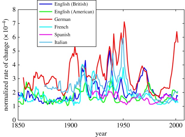
Rates of change for British English, American English, German, French, Spanish and Italian.

Next, we try to discern shared, universal tendencies. In figure 9, we compare the rates of change for respectively the kernel (as mentioned, the words that account for 75% of a given corpus) and the full lexicon across seven languages. The bar plots, which show changes over 10 and 50 year periods (using the periods specified in table 1), confirm our earlier finding that more frequent words—here, the kernel lexicon—are less prone to change than less frequent ones, with proportions of change in all versus kernel words looking somewhat similar across languages. The Pearson correlation coefficient between change in the kernel and the full lexicons across languages is r = 0.976 (p = 0.00018) for the 10 year intervals and r = 0.7995 (p = 0.031) for 50 year intervals. While these proportions, then, are similar across languages for both 10- and 50-year periods, the absolute rates of change only become similar across languages over larger time periods: the standard deviation in the rate of change for all words across languages drops from 1.100 × 10⁻⁴ to 0.566 × 10⁻⁴ when widening the interval from 10 to 50 years, and for the kernel words it drops from 1.122 × 10⁻⁴ to 0.446 × 10⁻⁴. These results suggest that once we broaden the horizon to wider time intervals, the effects of historically contingent changes cancel out, and languages begin to behave quite similarly.

5. Discussion and conclusion

The lexicon of a language reflects the world of its speakers. Accordingly, changes in the lexicon of a language reflect changes in the environment, understood in the broadest possible sense, of its users. The same goes for the frequencies or changes in frequencies of words. Several studies of frequency changes pertaining to individual words using the Google N-Gram Corpus confirm this [13,16,19–21]. The specificity and historically contingent nature of lexical change seemingly contradict observations regarding regularities underlying lexical change which cut across languages and time periods, i.e. universals of lexical change [1,2,9,10,17,18,24]. The contradiction, however, is only apparent, because the points of view are distinct. It is only in the bird's eye view, facilitated by either large amounts of data or large time spans, that regularities emerge.

Using an information-theoretic measure of frequency changes, we have found support for both a particularistic and a universalistic view of lexical change. Looking at individual languages like English, Russian, and other European languages, we clearly see that frequency distributions are sensitive to changes in society and historical events, even if it is only possible to discern the relationship for a few very important international events like the two world wars. In order to pursue this line of research further, it would be necessary to develop some independent index of information fluctuation in society to be correlated with the changes in lexical frequencies. This is a fascinating but daunting task which is beyond of the scope of this paper.

Lexical change is not only prompted by changes in the social and natural environments, but also by the particular linguistic environment, be it other languages or dynamics among different groups of speakers of one and the same language. In this paper, we have caught some glimpses of how the developments of American and British English are interrelated. From the point in time when sufficient data are available to us, i.e. 1840, to about a century later, we observe a steady divergence, a trend that must have begun already with the colonization of North America. By the mid-twentieth century, however, the two variants begin to converge, quite likely owing to the advent of mass media, including radio and television. Throughout the twentieth century, British English typically looks lexically like a slightly outdated version of American English, but in very recent years, the two variants seem to be moving more in tandem. These results show a situation in which the universal tendency for dialects to diverge into separate languages as they split up [26] is counteracted by historical circumstances that lead them to re-converge.

Looking at which words are more responsible for changes in frequency profiles, we have observed that more frequent words in English exhibit less variation in their frequencies over time. For English, the normalized change in frequency of a word over time is a power function of the word's frequency having an exponent of –0.316. There may well be a universal regularity here, and it would be interesting in future research to look at variability of the exponent across languages, as well as to investigate possible relations between this phenomenon and Zipf's law, which states that the frequency of a word is a power-law function of its frequency rank [24,27–30]. Meanwhile, the English data serve as a confirmation from at least one language that stability is inversely related to frequency, a finding that previously had been made based on a much more restricted set of lexical items [11]. Across languages, it is also the case that the rate of change is smaller for what we have called the ‘kernel lexicon’, namely those words which constitute 75% of the corpus representing a given language. For both the entire set of words and the kernel, the rate of change varies markedly across languages when observed within 10-year windows, but when the window is broadened to 50 year intervals, languages behave more similarly.

Swadesh [1], who first proposed the hypothesis that the rate of change is constant across a selected set of lexical items, measured lexical change over time in units of millennia. If the number of years and languages documented in the Google N-Gram Corpus were an order of magnitude larger, it is likely that we would find support for a version of Swadesh's hypothesis extended to the entire lexicon.

Funding statement

S.W.'s research was supported by an ERC advanced grant (MesAndLin(g)k, proj. no. 295918) and by a subsidy of the Russian Government to support the Programme of Competitive Development of Kazan Federal University.

References

- 1.Swadesh M. 1955. Towards greater accuracy in lexicostatistic dating. Int. J. Am. Ling. 21, 121–137. ( 10.1086/464321) [DOI] [Google Scholar]
- 2.Lees RB. 1953. The basis of glottochronology. Language 29, 113–127. ( 10.2307/410164) [DOI] [Google Scholar]
- 3.McMahon A, McMahon R. 2005. Language classification by numbers. Oxford, UK: Oxford University Press. [Google Scholar]
- 4.Heggarty P. 2010. Beyond lexicostatistics: how to get more out of ‘word list’ comparisons. Diachronica 27, 301–324. ( 10.1075/dia.27.2.07heg) [DOI] [Google Scholar]
- 5.Campbell L. 2004. Historical linguistics. An introduction. Edinburgh, UK: Edinburgh University Press. [Google Scholar]
- 6.Campbell L. 1997. American Indian languages. The historical linguistics of native America. Oxford, UK: Oxford University Press. [Google Scholar]
- 7.Burlak SA, Starostin SA. 2001. Vvedenie v lingvisticheskuju komparativistiku. Moscow, Russia: Editorial URSS. [Google Scholar]
- 8.Bergsland K, Vogt H. 1962. On the validity of glottochronology. Curr. Anthropol. 3, 115–153. ( 10.1086/200264) [DOI] [Google Scholar]
- 9.Holman EW, et al. 2011. Automated dating of the world's language families based on lexical similarity. Curr. Anthropol. 52, 841–875. ( 10.1086/662127) [DOI] [Google Scholar]
- 10.Holman EW, Wichmann S, Brown CH, Velupillai V, Müller A, Bakker D. 2008. Explorations in automated language classification. Folia Linguist. 42, 331–354. ( 10.1515/FLIN.2008.331) [DOI] [Google Scholar]
- 11.Pagel M, Atkinson QD, Meade A. 2007. Frequency of word-use predicts rates of lexical evolution throughout Indo-European history. Nature 449, 717–720. ( 10.1038/nature06176) [DOI] [PubMed] [Google Scholar]
- 12.Lieberman E, Michel J-B, Jackson J, Tang T, Nowak MA. 2007. Quantifying the evolutionary dynamics of language. Nature 449, 713–716. ( 10.1038/nature06137) [DOI] [PMC free article] [PubMed] [Google Scholar]
- 13.Michel J-B, et al. 2011. Quantitative analysis of culture using millions of digitized books. Science 331, 176–182. ( 10.1126/science.1199644) [DOI] [PMC free article] [PubMed] [Google Scholar]
- 14.Gao J, Hu J, Mao X, Perc M. 2012. Culturomics meets random fractal theory: insights into long-range correlations of social and natural phenomena over the past two centuries. J. R. Soc. Interface 9, 1956–1964. ( 10.1098/rsif.2011.0846) [DOI] [PMC free article] [PubMed] [Google Scholar]
- 15.Gerlach M, Altmann EG. 2013. Stochastic model for the vocabulary growth in natural languages. Phys. Rev. X 3, 021006 ( 10.1103/PhysRevX.3.021006) [DOI] [Google Scholar]
- 16.Perc M. 2012. Evolution of the most common English words and phrases over the centuries. J. R. Soc. Interface 9, 3323–3328. ( 10.1098/rsif.2012.0491) [DOI] [PMC free article] [PubMed] [Google Scholar]
- 17.Petersen AM, Tenenbaum J, Havlin S, Stanley HE. 2012. Statistical laws governing fluctuations in word use from word birth to word death. Sci. Rep. 2, 313 ( 10.1038/srep00313) [DOI] [PMC free article] [PubMed] [Google Scholar]
- 18.Petersen AM, Tenenbaum JN, Havlin S, Stanley HE, Perc M. 2012. Languages cool as they expand: allometric scaling and the decreasing need for new words. Sci. Rep. 2, 943 ( 10.1038/srep00943) [DOI] [PMC free article] [PubMed] [Google Scholar]
- 19.Bochkarev VV, Shevlakova AV, Solovyev VD. In press. Average word length dynamics as indicator of cultural changes in society. Soc. Evol. Hist. [Google Scholar]
- 20.Greenfield PM. 2013. The changing psychology of culture from 1800 through 2000. Psychol. Sci. 24, 1722–1731. ( 10.1177/0956797613479387) [DOI] [PubMed] [Google Scholar]
- 21.Oishi S, Graham J, Kesebir S, Costa Galinha I. 2013. Concepts of happiness across time and cultures. Pers. Soc. Psychol. Bull. 39, 559–577. ( 10.1177/0146167213480042) [DOI] [PubMed] [Google Scholar]
- 22.Lin Y, Michel J-B, Lieberman Aiden E, Orwant J, Brockman W, Petrov S. 2012. Syntactic annotations for the Google Books Ngram Corpus. In Proc. 50th Ann. Meeting Ass. Comput. Linguist., pp. 169–174, Jeju, Republic of Korea, 8–14 July 2012. [Google Scholar]
- 23.Kullback S, Leibler RA. 1951. On information and sufficiency. Ann. Math. Stat. 22, 79–86. ( 10.1214/aoms/1177729694.MR39968) [DOI] [Google Scholar]
- 24.Corominas-Murtra B, Fortuny J, Solé RV. 2011. Emergence of Zipf's law in the evolution of communication. Phys. Rev. E 83, 036115 ( 10.1103/PhysRevE.83.036115) [DOI] [PubMed] [Google Scholar]
- 25.Hughes JM, Foti NJ, Krakauer DC, Rockmore DN. 2012. Quantitative patterns of stylistic influence in the evolution of literature. Proc. Natl Acad. Sci. USA 109, 7682–7686. ( 10.1073/pnas.1115407109) [DOI] [PMC free article] [PubMed] [Google Scholar]
- 26.de Oliveira PMC, Sousa AO, Wichmann S. 2013. On the disintegration of (proto-)languages. Int. J. Sociol. Lang. 221, 11–19. ( 10.1515/ijsl-2013-0021) [DOI] [Google Scholar]
- 27.Zipf GK. 1936. The psycho-biology of language. London, UK: Routledge. [Google Scholar]
- 28.Baayen RH. 2001. Word-frequency distributions. Dordrecht, The Netherlands: Springer-Science + Business Media, B.V. [Google Scholar]
- 29.Ferrer I Cancho R. 2005. The variation of Zipf's law in human language. Eur. Phys. J. B 44, 249–257. ( 10.1140/epjb/e2005-00121-8) [DOI] [Google Scholar]
- 30.Ángeles Serrano M, Flammini A, Menczer F. 2009. Modeling statistical properties of written text. PLoS ONE 4, e5372 ( 10.1371/journal.pone.0005372) [DOI] [PMC free article] [PubMed] [Google Scholar]
Associated Data
This section collects any data citations, data availability statements, or supplementary materials included in this article.