An efficient and unbiased method for sensitivity analysis of stochastic reaction networks

Abstract

We consider the problem of estimating parameter sensitivity for Markovian models of reaction networks. Sensitivity values measure the responsiveness of an output with respect to the model parameters. They help in analysing the network, understanding its robustness properties and identifying the important reactions for a specific output. Sensitivity values are commonly estimated using methods that perform finite-difference computations along with Monte Carlo simulations of the reaction dynamics. These methods are computationally efficient and easy to implement, but they produce a biased estimate which can be unreliable for certain applications. Moreover, the size of the bias is generally unknown and hence the accuracy of these methods cannot be easily determined. There also exist unbiased schemes for sensitivity estimation but these schemes can be computationally infeasible, even for very simple networks. Our goal in this paper is to present a new method for sensitivity estimation, which combines the computational efficiency of finite-difference methods with the accuracy of unbiased schemes. Our method is easy to implement and it relies on an exact representation of parameter sensitivity that we recently proved elsewhere. Through examples, we demonstrate that the proposed method can outperform the existing methods, both biased and unbiased, in many situations.

1. Introduction

Reaction networks are frequently encountered in several scientific disciplines, such as chemistry [1], systems biology [2], epidemiology [3], ecology [4] and pharmacology [5]. It is well known that when the population sizes of the reacting species are small, then a deterministic formulation of the reaction dynamics is inadequate for understanding many important properties of the system [6,7]. Hence, stochastic models are necessary and the most prominent class of such models is where the reaction dynamics is described by a continuous time Markov chain (CTMC). Our paper is concerned with sensitivity analysis of these Markovian models of reaction networks.

Generally, reaction networks involve many kinetic parameters that influence their dynamics. With sensitivity analysis, one can measure the receptiveness of an outcome to small changes in parameter values. These sensitivity values give insights about network design and its robustness properties [8]. They also help in identifying the important reactions for a given output, estimating the model parameters and in fine-tuning the system's behaviour [9]. The existing literature contains many methods for sensitivity analysis of CTMC models, but all these methods have certain drawbacks. They introduce a bias in the sensitivity estimate [10–13] or the associated estimator can have large variances [14] or the method becomes impractical for large networks [15]. Owing to these reasons, the search for better methods for sensitivity analysis of stochastic reaction networks is still an active research problem.

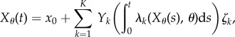
Consider a stochastic reaction network consisting of d species S₁, … , S_d. Under the well-stirred assumption [16], the state of the system at any time is given by a vector in , where is the set of non-negative integers. When the state is x = (x₁, … , x_d), then the population size corresponding to species S_i is x_i. The state evolves as the species interact through K reaction channels. If the state is x, then the kth reaction fires at rate λ_k(x) and it displaces the state by the stoichiometric vector . Here, λ_k is called the propensity function for the kth reaction. We can represent the reaction dynamics by a CTMC and the distribution of this process evolves according to the Chemical Master Equation [16] which is quite difficult to solve except in some restrictive cases. Fortunately, the sample paths of this process can be easily simulated using Monte Carlo procedures such as Gillespie's stochastic simulation algorithm (SSA) and its variants [16,17].

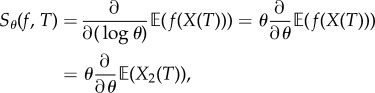
Suppose that the propensity functions of a reaction network depend on a scalar parameter θ. Hence, when the state is x, the kth reaction fires at rate λ_k(x, θ). Let denote the CTMC representing the reaction dynamics with a known initial state x₀. For a function and an observation time T ≥ 0, our output of interest is f(X_θ(T)). We determine how much the expected value of this output changes with infinitesimal changes in the parameter θ. In other words, our aim is to compute

1.1

Since the mapping 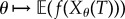is generally unknown, it is difficult to evaluate S_θ(f, T) directly. Therefore, we need to estimate this quantity using simulations of the process X_θ. For this purpose, many methods use a finite-difference scheme such as

1.2

for a small h. These methods reduce the variance of the associated estimator by coupling the processes X_θ and X_θ+h in an intelligent way. Three such couplings are: common reaction numbers (CRN) [11], common reaction paths (CRP) [11] and coupled finite differences (CFD) [13]. The two best-performing finite-difference schemes are CRP and CFD, and we shall discuss them in §2.1. It is immediate that a finite-difference scheme produces a biased estimate of the true sensitivity value S_θ(f, T). To further compound this problem, the size and even the sign of the bias is unknown in most cases, thereby casting a doubt over the estimated sensitivity values. The magnitude of the bias must be proportional to h, but it can still be significant for small h (see §4). One can reduce the bias by decreasing h, but as h gets smaller, the variance of the finite-difference estimator gets larger, making it necessary to generate an extremely large sample to obtain a statistically accurate estimate. In many cases, for small values of h, the computational cost of generating a large sample is so high that finite-difference schemes become inefficient in comparison to the unbiased methods. Unfortunately, there is no way to select an optimum value of h, which is small enough to ensure that the bias is small and simultaneously large enough to ensure that the estimator variance is low. This is the main difficulty in using finite-difference schemes and we shall revisit this point in §4.

To obtain highly accurate estimates of S_θ(f, T), we need unbiased methods for sensitivity analysis. The first such scheme is the likelihood-ratio method which relies on the Girsanov measure transformation [14,18]. Hence, we refer to it as the Girsanov method in this paper. In this method, the sensitivity value is expressed as

1.3

where s_θ(f, t) is a random variable whose realizations can be easily obtained by simulating the CTMC X_θ in the time interval [0, T]. The Girsanov method is easily implementable, and its unbiasedness guarantees convergence to the right value S_θ(f, T) as the sample size tends to infinity. However in many situations, the estimator associated with this method has a very high variance, making it extremely inefficient [11–13,15]. To remedy this problem, we proposed another unbiased scheme in [15] based on a different sensitivity formula of the form (1.3), which is derived using the random time-change representation of Kurtz (see ch. 7 in [19]). Unfortunately in this formula, the realizations of s_θ(f, T) cannot be easily computed from the paths of the process X_θ as it involves several expectations of functions of the underlying CTMC at various times and various initial states. If all these expectations are estimated serially using independent paths, then the problem becomes computationally intractable. Hence, we devised a scheme in [15], called the Auxiliary Path Algorithm (APA), to estimate all these expectations in parallel using a fixed number of auxiliary paths. The implementation of APA is quite difficult and the memory requirements are high because one needs to store the paths and dynamically maintain a large table to estimate the relevant quantities. These reasons make APA impractical for large networks and also for large observation times T. However, in spite of these difficulties, we showed in [15] that APA can be far more efficient than the Girsanov method in certain situations.

The above discussion suggests that all the existing methods for sensitivity analysis, both biased and unbiased, have certain drawbacks. This motivated us to develop a new method for sensitivity estimation which is unbiased, easy to implement, has low memory requirements and is more versatile than the existing unbiased schemes. We use the main result in [15] to construct another random variable such that (1.3) holds. We then provide a simple scheme, called the Poisson path algorithm (PPA), to obtain realizations of and this gives us a method to obtain unbiased estimates of parameter sensitivities for stochastic reaction networks. Similar to APA, PPA also requires estimation of certain quantities using auxiliary paths, but the number of these quantities can be controlled to be so low that they can be estimated serially using independent paths. Consequently, PPA does not require any storage of paths or the dynamic maintenance of a large table as in APA. Hence, the memory requirements are low, the implementation is easier and PPA works well for large networks and for large observation times T. In §4, we consider many examples to compare the performance of PPA with the Girsanov method, CFD and CRP. We find that PPA is usually far more efficient than the Girsanov method. Perhaps surprisingly, in many situations PPA can also outperform the finite-difference schemes (CRP and CRN) if we impose the restriction that the bias is small. This makes PPA an attractive method for sensitivity analysis because one can efficiently obtain sensitivity estimates, without having to worry about the (unknown) bias caused by finite-difference approximations.

This paper is organized as follows. In §2, we provide the relevant mathematical background and discuss the existing schemes for sensitivity analysis in greater detail. We also present our main result which shows that for a suitably defined random variable , relation (1.3) is satisfied. In §3, we describe PPA which is a simple method to obtain realizations of . In §4, we consider many examples to illustrate the efficiency of PPA and compare its performance with other methods. Finally, in §5, we conclude and discuss future research directions.

2. Preliminaries

Recall the description of the reaction network from the previous section and suppose that the propensity functions depend on a real-valued parameter θ. We can model the reaction dynamics by a CTMC whose generator¹ is given by

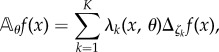where is any bounded function and 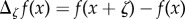. Under some mild conditions on the propensity functions (see Condition 2.1 in [15]), a CTMC (X_θ(t))_t≥0 with generator and any initial state x₀ exists uniquely. The random time-change representation of Kurtz (see ch. 7 in [19]) shows that this CTMC can be expressed as

2.1

where is a family of independent unit rate Poisson processes.

In this paper, we are interested in computing the sensitivity value S_θ(f, T) defined by (1.1). Assume that we can express the sensitivity value as (1.3) for some random variable s_θ(f, T). If we are able to generate N independent samples from the distribution of s_θ(f, T), then S_θ(f, T) can be estimated as

2.2

which is a random variable with mean μ_N and variance given by

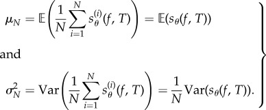2.3

Owing to the central limit theorem, for large values of N, the distribution of is approximately normal with mean μ_N and variance . Hence, for any interval , the probability can be approximated as

2.4

where is the cumulative distribution function for the standard normal distribution and σ_N is the standard deviation. Generally, μ_N and σ_N are unknown but they can be estimated from the sample as

Note that the mean μ_N is just the one-point estimate for the sensitivity value, while the standard deviation σ_N measures the statistical spread around μ_N. The standard deviation σ_N can also be seen as the estimation error. From (2.3), it is immediate that σ_N is directly proportional to Var(s_θ(f, T)) but inversely proportional to N. Hence, if Var(s_θ(f, T)) is high then a larger number of samples is needed to achieve a certain statistical accuracy.

In finite-difference schemes, instead of S_θ(f, T) one estimates a finite difference S_θ,h(f, T) of the form (1.2) which can be written as for

2.5

Here, the Markov processes X_θ and X_θ+h are defined on the same probability space and they have generators and , respectively. In this case, the estimator mean μ_N and variance are given by (2.3) with s_θ(f, T) replaced by s_θ,h(f, T).

2.1. Finite-difference schemes

The main idea behind the various finite-difference schemes is that by coupling the processes X_θ and X_θ+h, one can increase the covariance between f(X_θ+h(T)) and f(X_θ(T)), thereby reducing the variance of s_θ,h(f, T) and making the estimation procedure more efficient. As mentioned before, three such couplings suggested in the existing literature are: CRN [11], CRP [11] and CFD [13]. Among these, we only consider the two best-performing schemes, CRP and CFD, in this paper.

In CRP, the processes X_θ and X_θ+h are coupled by their random time-change representations according to

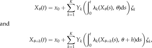where is a family of independent unit rate Poisson processes. Note that these Poisson processes are the same for both processes X_θ and X_θ+h, indicating that their reaction paths are the same.

In CFD, the processes X_θ and X_θ+h are coupled by their random time-change representations as

and

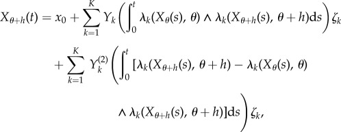where and is again a family of independent unit rate Poisson processes. Under this coupling, the processes X_θ and X_θ+h have the same state until the first time the counting process corresponding to or fires for some k. The probability that this separation time will come before T is proportional to h, which is usually small. This suggests that the processes X_θ and X_θ+h are strongly coupled.

Note that both CRP and CFD are estimating the same quantity S_θ,h(f, T) (1.2) and hence they both suffer from the same bias . The only difference between them is in the coupling of the processes X_θ and X_θ+h, which alters the variance of s_θ,h(f, T). For a given example, the method with a lower variance is more efficient as it requires a smaller sample to achieve the desired statistical accuracy.

For a finite-difference scheme of the form (1.1), the bias is of order h. However, replacing θ by (θ − h/2), we obtain a centred finite-difference scheme which has a bias of order h². Such a centring does not cause any additional difficulties in simulating the coupled processes for CFD or CRN, but it may lead to a bias which is substantially smaller. Therefore, for the purpose of comparison, we work with the centred versions of CFD and CRN in this paper. In particular, we simulate processes X_(θ−h/2) and X_(θ+h/2) according to the appropriate coupling mechanism and estimate sensitivity as 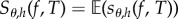, where

2.6

One can show that the variance Var(s_θ,h(f, T)) of the random variable s_θ,h(f, T) is proportional to 1/h. Hence, by making h smaller, we may reduce the bias but we will have to pay a computational cost by generating a large number of samples for the required estimation. This trade-off between bias and efficiency is the major drawback of finite-difference schemes as one generally does not know the right value of h for which S_θ,h(f, T) is close enough to S_θ(f, T), while the variance of s_θ,h(f, T)) is not too large.

2.2. Unbiased schemes

Unbiased schemes are desirable because one does not have to worry about the bias, and the accuracy of the estimate can be improved by simply increasing the number of samples. The Girsanov method is the first such unbiased scheme [14,18] for sensitivity estimation. Recall the random time-change representation (2.1) of the process (X_θ(t))_t≥0. In the Girsanov method, we express S_θ(f, T) as (1.3) where

2.7

and (R_k(t))_t≥0 is the counting process given by

In (2.7), R_k(dt) = 1 if and only if the kth reaction fires at time t. For any other t, R_k(dt) = 0. Hence, if the kth reaction fires at times in the time interval [0, T], then

The Girsanov method is simple to implement because realizations of s_θ(f, T) can be easily generated by simulating the paths of the process X_θ until time T. However, as mentioned before, the variance of s_θ(f, T) can be very high [11–13], which is a serious problem as it implies that a large number of samples are needed to produce statistically accurate estimates. As simulations of the process X_θ can be quite cumbersome, generating a large sample can take an enormous amount of time.

Now consider the common situation where we have mass–action kinetics and θ is the rate constant of reaction k₀. Then has the form and for every k ≠ k₀, λ_k does not depend on θ. In this case, the formula (2.7) for s_θ(f, T) simplifies to

2.8

where is the number of times reaction k₀ fires in the time interval [0, T]. Clearly, the Girsanov method cannot estimate the sensitivity value at θ = 0 even though S_θ(f, T) (1.1) is well defined. This is a big disadvantage as the sensitivity value at θ = 0 is useful for understanding network design as it informs us whether the presence or absence of reaction k₀ influences the output or not. Unfortunately, the problem with the Girsanov method is not just limited to θ = 0. Even for θ close to 0, the variance of s_θ(f, T) can be very high, rendering this method practically infeasible [15]. This is again a serious drawback as reaction rate constants with small values are frequently encountered in systems biology and other areas.

These issues with the Girsanov method severely restrict its use and also highlight the need for new unbiased schemes for sensitivity analysis. In our recent paper [15], we provide a new unbiased scheme based on another sensitivity formula of the form (1.3). To motivate this formula, we first discuss the problem of computing parameter sensitivity in the deterministic setting.

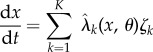
Consider the deterministic model for the parameter-dependent reaction network with reaction flux [20] and propensity vector ζ_k for reaction k. If denotes the vector of species concentrations at time t, then (x_θ(t))_t≥0 is the solution of the following system of ordinary differential equations:

2.9

with initial condition x(0) = x₀. Pick an observation time T > 0 and a differentiable output function , and suppose we are interested in computing the sensitivity value

Using (2.9) we can write

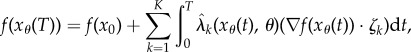where denotes the gradient of the map and · denotes the standard inner product on . Assuming differentiability of 's we get

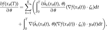2.10

where can be easily computed by solving the ordinary differential equation obtained by differentiating (2.9) with respect to θ. Hence, in the deterministic setting, computation of the parameter sensitivity is relatively straightforward.

Relation (2.10) helps us in viewing parameter sensitivity as the sum of two parts: sensitivity of the reaction fluxes and the sensitivity of the states x_θ(t). In [15], we provide such a decomposition for parameter sensitivity in the stochastic setting. However, unlike the deterministic scenario, measuring the second contribution is computationally very challenging. In order to present this result, we need to define certain quantities. Let (X_θ(t))_t≥0 be a CTMC with generator . For any , t ≥ 0, k = 1, … , K and define

2.11

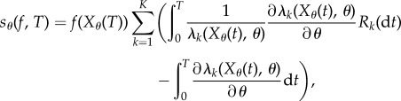
Define and let σ₀, σ₁, σ₂ denote the successive jump times² of the process X_θ. Theorem 2.3 in [15] shows that S_θ(f, T) satisfies (1.3) with

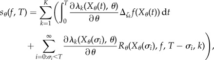2.12

where

2.13

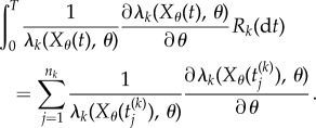
This result was proved by coupling the processes X_θ and X_θ+h as in CFD (see §2.1) and computing the limit of the finite difference S_θ,h(f, T) (see (1.2)) as h → 0. Similar to the deterministic case, this result shows that parameter sensitivity S_θ(f, T) can be seen as the sum of two parts: the sensitivity of the propensity functions (λ_k) and the sensitivity of the states X_θ(σ_i) of the Markov process at the jump times σ_i. Computing the latter contribution is difficult because it involves the function R_θ which generally does not have an explicit formula. To overcome this problem, one needs to estimate all the quantities of the form R_θ(x, f, t, k) that appear in (2.12). However, the number of these quantities is proportional to the number of jumps of the process before time T, which can be quite high even for small networks. If we estimate each of these quantities serially, as and when they appear, using a collection of independently generated paths of the process X_θ, then the problem becomes computationally intractable for most examples of interest. In [15], we devised a scheme, called the APA, to estimate all these quantities in parallel by generating a fixed number of auxiliary paths in addition to the main path. APA stores information about all the required quantities in a big Hashtable and tracks the states visited by the auxiliary paths to estimate those quantities. Owing to all the necessary book-keeping, APA is hard to implement and it also has high memory requirements. In fact, the space and time complexity of APA scales linearly with the number of jumps in the time interval [0, T] and this makes APA practically unusable for large networks or for large values of observation time T. Moreover, APA only works well if the stochastic dynamics visits the same states again and again, which may not be generally true.

The above discussion suggests that if we can modify the expression for s_θ(f, T) in such a way that only a small fraction of unknown quantities (of the form R_θ(x, f, t, k)) require estimation, then it can lead to an efficient method for sensitivity estimation. We exploit this idea in this paper. By adding extra randomness to the random variable s_θ(f, T), we construct another random variable , which has the same expectation as s_θ(f, T)

2.14

even though its distribution may be different. We then show that realizations of the random variable can be easily obtained through a simple procedure. This gives us a new method for unbiased parameter sensitivity estimation for stochastic reaction networks.

2.3. Construction of

We now construct the random variable introduced in the previous section. Let (X_θ(t))_t≥0 be the CTMC with generator and initial state x₀. Let σ₀, σ₁, … denote the successive jump times of this process. The total number of jumps until time T is given by

2.15

For any T > 0, we have η ≥ 1 because σ₀ = 0. If the process X_θ reaches a state x for which λ₀(x, θ) = 0, then x is an absorbing state and the process stays in x forever. From (2.15), it is immediate that for any non-negative integer i < η, X_θ(σ_i) cannot be an absorbing state. Let α indicate if the final state X_θ(σ_η) is absorbing

For each i = 0, … , (η − α), let γ_i be an independent exponentially distributed random variable with rate λ₀(X_θ(σ_i), θ) and define

For each i = 0, … , (η − α) and k = 1, … , K, let β_ki be given by

where

Fix a normalizing constant c > 0. The choice of c and its role will be explained later in the section. If β_ki≠ 0 and Γ_i = 1, then let be an independent -valued random variable whose distribution is Poisson with parameter

2.16

Here, the denominator λ₀(X_θ(σ_i), θ) is non-zero because for i ≤ (η − α) the state X_θ(σ_i) cannot be absorbing. On the event , we define another random variable as

2.17

where (Z₁(t))_t≥0 and (Z₂(t))_t≥0 are two processes which are coupled by the following random time-change representations:

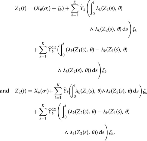where is an independent family of unit rate Poisson processes. This coupling is similar to the coupling used by CFD (see §2.1). Note that (Z₁(t))_t≥0 and (Z₂(t))_t≥0 are Markov processes with generator and initial states (X_θ(σ_i) + ζ_k) and X_θ(σ_i), respectively. Therefore,

2.18

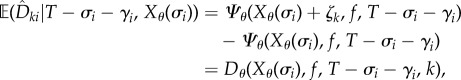
where D_θ is defined by (2.11). In other words, given T − σ_i − γ_i = t and X_θ(σ_i) = x, the mean of the random variable is just D_θ(x, f, t, k). The above coupling between (Z₁(t))_t≥0 and (Z₂(t))_t≥0 makes them strongly correlated, thereby lowering the variance of the difference . This strong correlation is evident from the fact that if Z₁(s) = Z₂(s) for some s ≥ 0 then Z₁(u) = Z₂(u) for all u ≥ s. Finally, if the last state X_θ(σ_η) is absorbing (that is, α = 1) and ∂λ_k(X_θ(σ_η), θ)/∂θ is non-zero, then we define another random variable as

2.19

where (Z(t))_t≥0 is an independent Markov process with generator and initial state X_θ(σ_η) + ζ_k. Note that

2.20

We are now ready to provide an expression for . Let

and define

2.21

By a simple conditioning argument, we prove in the electronic supplementary material, §1, that relation (2.14) holds.

At first glance, it seems that obtaining realizations of suffers from the same difficulties as obtaining realizations of s_θ(f, T), because at each jump time σ_i < T, one needs to compute an unknown quantity which requires simulation of new paths of the process X_θ. However, note that is only needed if the Poisson random variable is strictly positive. Therefore, if we can effectively control the number of positive 's, then we can efficiently generate realizations of . This can be achieved using the positive parameter c (see (2.16)) as we later explain. The construction of outlined above also provides a recipe for obtaining its realizations. Hence, we have a method for estimating the parameter sensitivity S_θ(f, T). We call this method the PPA because at each jump time σ_i, the crucial decision of whether new paths of the process X_θ are needed (for ) is based on the value of a Poisson random variable . We describe PPA in greater detail in §3.

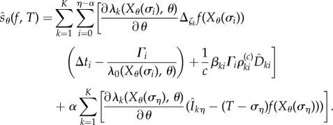
We now discuss how the positive parameter c can be selected. Let η_req denote the total number of positive 's that appear in (2.21). This is the number of 's that are required to obtain a realization of . It is immediate that η_req is bounded above by , which is a Poisson random variable with parameter cR_tot, where

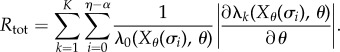2.22

By picking a small c > 0, we can ensure that is small, which would also guarantee that ρ_tot and η_req are small. Specifically, we choose a small positive integer M₀ (like 10, for instance) and set

2.23

where is estimated using N₀ simulations of the process X_θ in the time interval [0, T]. The choice of N₀ is not critical and typically a small value (like 100, for example) is sufficient to provide a decent estimate of . The role of parameter M₀ is also not very important in determining the efficiency of PPA. If M₀ increases, then η_req increases as well, and the computational cost of generating each realization of becomes higher. However, as η_req increases, the variance of decreases and hence fewer realizations of are required to achieve the desired statistical accuracy. These two effects usually offset each other and the overall efficiency of PPA remains relatively unaffected. Note that PPA provides unbiased estimates for the sensitivity values, regardless of the choice of N₀ and M₀.

3. The Poisson path algorithm

We now describe PPA which produces realizations of the random variable (defined by (2.21)) for some observation time T and some output function f. Since , we can estimate S_θ(f,T) by generating N realizations of the random variable and then computing their empirical mean (2.2).

Let x₀ denote the initial state of the process X_θ and assume that the function rand() returns independent samples from the uniform distribution on [0,1]. We simulate the paths of our CTMC using Gillespie's SSA [16]. When the state is x, the next time increment (Δt) and reaction index (k) is given by the function SSA(x) (see the electronic supplementary material, algorithm 1 in §2). We first fix a normalization parameter c according to (2.23), by estimating using N₀ simulations of the CTMC (see the electronic supplementary material, algorithm 2 in §2).

Once c is chosen, a single realization of can be computed using GenerateSample(x₀, T, c) (algorithm 1). This method simulates the process X_θ according to SSA and at each state x and jump time t, the following happens:

• — If x is an absorbing state (λ₀(x, θ) = 0), then t is the last jump time before T (t = σ_η). For each k = 1, … , K such that ∂λ_k(x, θ)/∂θ ≠ 0, the quantity (see (2.19)) is evaluated using EvaluateIntergal(x + ζ_k, T − t) (see the electronic supplementary material, algorithm 3 in §2) and then used to update the sample value according to (2.21).

• — If x is not an absorbing state, then t = σ_i for some jump time σ_i with i < η. An exponential random variable γ (where γ = γ_i in (2.21)) is generated, and for each k = 1, … , K such that ∂λ_k(x, θ)/∂θ ≠ 0, the Poisson random variable n (where in (2.21)) is also generated. If γ < (T − t) and n > 0, then the quantity (see (2.17)) is evaluated using EvaluateCoupledDifference(x, x + ζ_k, T − t − γ) (see the electronic supplementary material, algorithm 5 in §2) and then used to update the sample value according to (2.21). A Poisson random variable with parameter r is generated using the function GeneratePoisson(r) (see the electronic supplementary material, algorithm 4 in §2).

4. Numerical examples

In this section, we present many examples to compare the performance of PPA with the Girsanov method which is unbiased, and the two best-performing finite-difference schemes, CFD and CRP, which are of course biased. To compare the performance of different methods, we compare the time they need to produce a statistically accurate estimate of the true sensitivity value S_θ(f, T) given by (1.1). Our first task is to find a way to judge that an estimate of S_θ(f, T) is statistically accurate.

A common way to assess statistical accuracy of an estimator (biased or unbiased) is by computing its mean-squared error (m.s.e.), which is the sum of its variance and its bias (squared). However m.s.e. is not well-suited for our situation. To see this, consider two sensitivity estimators whose means are μ₁ = 2 and μ₂ = 1.1, and standard deviations are σ₁ = 0.1 and σ₂ = 1. Assuming that the true sensitivity value is s₀ = 1 and the distribution of the estimators is approximately normal, the two estimators have the same m.s.e., which is equal to . However, the second estimator is clearly more accurate than the first one, because it is far more likely to yield a sensitivity estimate which is ‘close’ to the actual value s₀. This explains how m.s.e. can be misleading and therefore we now describe another method to compare the statistical accuracy of estimators.

Algorithm 1. Generates one realization of according to (2.21).
1:	function GenerateSample(x0, T, c)
2:	Set x = x0, t = 0 and s = 0
3:	while t < T do
4:	Calculate (Δt, k0) = SSA(x)
5:	Update Δt ← min{Δt, T − t}
6:	if λ0(x, θ) > 0 then
7:	Set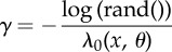
8:	end if
9:	for k = 1 to K do
10:	Set and
11:	if r > 0 then
12:	if λ0(x, θ) = 0 then
13:	Update (EvaluateIntegral
14:	else
15:	Set n = GeneratePoisson
16:	if γ < (T − t) then
17:	Update
18:	if n > 0 then
19:	Update EvaluateCoupledDifference
20:	end if
21:	else
22:
23:	end if
24:	end if
25:	end if
26:	end for
27:	Update t ← t + Δt and x ← x + ζk0
28:	end while
29:	return s
30:	end function

Suppose that a method estimates parameter sensitivity using N samples whose mean is μ_N and standard deviation is σ_N (see §2). Assume that the true value of S_θ(f, T) is s₀. Let and , where denotes the absolute value function. Then [a, b] is the 5% interval around the true value s₀. Under the central limit approximation, the estimator can be seen as a normally distributed random variable with mean μ_N and variance . Hence, using (2.4) we can calculate the probability

that the estimator lies within the 5% interval around s₀. Henceforth, we refer to p as the confidence level for the estimator. The statistical accuracy of an estimate can be judged from the value of p: the higher the value of p, the more accurate is the estimate. As we calculate p using the 5% interval around s₀, we ensure that the statistical precision is high or low depending on whether the sensitivity value is small or large.

The standard deviation σ_N is inversely proportional to the number of samples N (see §2), which shows that σ_N → 0 as N → ∞. For an unbiased scheme (Girsanov and PPA), we have μ_N → s₀ as N → ∞, due to the law of large numbers and therefore (2.4) implies that the confidence level p can be made as close to 1 as desired by picking a large sample size N. However, the same is not true for finite-difference schemes such as CFD and CRP. In such schemes, μ_N → S_θ,h(f, T) as N → ∞, where S_θ,h(f, T) is generally different from S_θ(f, T) = s₀ because of the bias. If this bias is large, then S_θ,h(f, T) may lie outside the 5% interval [a, b] around s₀, and hence p is close to 0 for large N. Therefore, if high confidence levels are desired with finite-difference schemes, then a small h must be chosen to ensure that the bias is low. However, the variance of the associated estimator scales as 1/h (see §2.1), implying that if h is too small then an extremely large sample size is required to achieve high confidence levels, and this can impose a heavy computational burden.

In this paper, we compare the efficiency of different methods by measuring the CPU time³ that is needed to produce a sample with least possible size, such that the corresponding estimate has a certain threshold confidence level. This threshold confidence level is close to 1 (either 0.95 or 0.99) and hence the produced estimate is statistically quite accurate. Previous discussion suggests that for finite-difference schemes, there is a trade-off between the statistical accuracy and the computational burden. This trade-off is illustrated in figure 1 which depicts four cases that correspond to four values of h arranged in decreasing order. We describe these cases below.

• Case 1. Here, h is large and so the computational burden is low. However, due to the large bias, the estimator distribution (normal curve in figure 1) puts very little mass on the 5% interval around the true sensitivity value. Therefore, the confidence level p is low and the estimate is unacceptable.

• Case 2. Now h is smaller, the computational burden is higher and the bias is lower. However, the estimator distribution still does not put enough mass on the 5% interval and so the value of p is not high enough for the estimate to be acceptable.

• Case 3. Now h is even smaller and so the computational burden is higher, but fortunately the bias is small enough to ensure that the estimator distribution puts nearly all its mass on the 5% interval. Therefore, the confidence level p is close to 1 and the estimate is acceptable.

• Case 4. Here, h is smallest and so the computational burden is the highest among all the cases. However in comparison to Case 3, the additional computational burden is unnecessary because there is only a slight improvement in the bias and the confidence level.

Figure 1.

Trade-off between accuracy and computational burden for finite-difference schemes. The four cases correspond to four values of h arranged in decreasing order. For Case 2, should be interpreted as ‘p is far away from 0 and 1’.

To use a finite-difference scheme efficiently, we need to know the largest value of h for which an estimate with a high confidence level can be produced (Case 3 in figure 1). However, in general, it is impossible to determine this value of h. A blind choice of h is likely to correspond to Cases 1 or 4 in figure 1. To make matters worse, since the true sensitivity value S_θ(f, T) is usually unknown, one cannot measure the statistical accuracy without re-estimating S_θ(f, T) using an unbiased method. Most practitioners who use finite-difference schemes assume that the statistical accuracy is high if h is small. However, this is not true in general (see example 4.1). Therefore, if high accuracy is desired, then an unbiased method should be preferred over finite-difference schemes.

As it is difficult to determine the optimum value of h, we adopt the following strategy to gauge the efficiency of a finite-difference scheme. We find the largest value of h in the sequence 0.1, 0.01, 0.001 … , for which the threshold confidence level p is achievable for a large enough sample size. For performance comparison, we only use the CPU time corresponding to this value of h and we disregard all the CPU time wasted in testing other values of h. We have intentionally made our comparison strategy more lenient towards the finite-difference schemes, in order to compensate for the arbitrariness in choosing the ‘test’ values of h.

To compute the confidence level p, we require the exact sensitivity value S_θ(f, T). In some examples, S_θ(f, T) can be analytically evaluated and the computation of p is straightforward. In other examples, where S_θ(f, T) cannot be explicitly computed, we use PPA to produce an estimate with a very low sample variance and since PPA is unbiased, this estimate would be close to the true sensitivity value S_θ(f, T) and hence it can be used in the calculation of p.

We now discuss the examples. In all the examples, the propensity functions λ_k follow mass–action kinetics unless stated otherwise. Our method PPA depends on two parameters N₀ and M₀ (see §2.3) and in this paper we always use N₀ = 100 and M₀ = 10. In each example, we provide a bar chart with the CPU times required by different methods to produce an estimate with the desired confidence level p = 0.95 or p = 0.99. This facilitates an easy performance comparison between various methods. The exact values of the CPU times, sample size N, estimator mean μ_N, estimator standard derivation σ_N and h (for finite-difference schemes) are provided in the electronic supplementary material, §3.

Example 4.1. (Single-species birth–death model) —

Our first example is a simple birth–death model in which a single species is created and destroyed as

Let θ₁ = θ₂ = 0.1 and assume that the sensitive parameter is θ = θ₂. Suppose that X(0) = 0 and let (X(t))_t≥0 be the CTMC representing the reaction dynamics. Hence the population of at time t is . For f(x) = x, we wish to estimate

for T = 20 and 100. As the propensity functions of this network are affine, we can compute S_θ(f, T) exactly (see the electronic supplementary material, §3) and use this value in computing the confidence level p of an estimate. We estimate S_θ(f, T) with all the methods with two threshold confidence levels (p = 0.95 and p = 0.99) and plot the corresponding CPU times in figure 2. For CFD and CRP, the desired confidence level was achieved in all the cases for h = 0.01.

Figure 2.

Efficiency comparison for birth–death model with two threshold confidence levels: p = 0.95 (a) and p = 0.99 (b) and two observation times: T = 20 and T = 100. The exact CPU time is shown at the top of each bar. Note that efficiency is inversely related to the CPU time. For finite-difference schemes, h = 0.01 was used in all the cases.

From figure 2, it is immediate that PPA generally performs better than the other methods. To measure this gain in performance more quantitatively, we compute the average speed-up factor of PPA with respect to other methods. For each threshold confidence level, this factor is calculated by simply taking the ratio of the aggregate CPU times required by a certain method and PPA to perform all the sensitivity estimations. In this example, this aggregate involves the CPU times for T = 20 and T = 100. These average speed-up factors are presented in table 1. Note that in this example, PPA is significantly faster than CRP but only slightly faster than CFD and the Girsanov method.

Table 1.

Birth–death model: average speed-up factors of PPA with respect to other methods.

p	Girsanov	CFD	CRP
0.95	2.16	1.75	8.59
0.99	1.5	1.22	7.25

Now we use this example to demonstrate the pitfalls of choosing a ‘wrong’ value of h for finite-difference schemes. We know from figure 2 that for T = 100, the desired confidence level of 0.99 was achieved with h = 0.01. This ‘right’ value of h corresponds to Case 3 in figure 1. If we select a higher value of h, such as h = 0.1 or h = 0.05, then with 10 000 samples we see that the achieved confidence level p is much lower than the desired value 0.99 (table 2), indicating that the estimate is not sufficiently accurate. Note that h = 0.1 and h = 0.05 correspond to Cases 1 and 2 in figure 1. Observe that for h = 0.1, the estimate produced by finite-difference schemes (μ_N) is more than 30% off from the exact sensitivity value of −9.995, which shows that the bias can be large for h that appears small. On the other hand, if we select h which is really small, such as h = 0.001, then we do produce an estimate with the desired confidence level of 0.99 (see table 2), but the required sample size is very large and hence the computational burden is much higher than the ‘right’ value of h, which is h = 0.01. The value h = 0.001 corresponds to Case 4 in figure 1.

Table 2.

Birth–death model: pitfalls of choosing a ‘wrong’ h.

h	method	N	mean (μN)	s.d. (σN)	CPU time (s)	p
0.1	CFD	−13.286	0.0998	10000	0.15	0
	CRP	−13.144	0.1206	10000	0.62	0
0.05	CFD	−10.634	0.1168	10000	0.13	0.1165
	CRP	−10.558	0.1504	10000	0.64	0.3370
0.001	CFD	−9.9424	0.1869	281723	3.65	0.99
	CRP	−10.0625	0.1829	300721	19.8	0.99

Example 4.2. (Gene expression network) —

Our second example considers the model for gene transcription given in [2]. It has three species, Gene (G), mRNA (M) and protein (P), and there are four reactions given by

The rate of translation of a gene into mRNA is θ₁, while the rate of transcription of mRNA into protein is θ₂. The degradation of mRNA and protein molecules occurs at rates θ₃ and θ₄, respectively. Typically, implying that a protein molecule lives much longer than a mRNA molecule. In accordance with the values given in [2] for lacA gene in bacterium E. coli, we set θ₁ = 0.6 min⁻¹, θ₂ = 1.7329 min⁻¹ and θ₃ = 0.3466 min⁻¹. Our sensitive parameter is θ = θ₄.

Let (X(t))_t≥0 be the CTMC representing the dynamics with initial state (X₁(0), X₂(0)) = (0, 0). For any time t, X(t) = (X₁(t), X₂(t)), where X₁(t) and X₂(t) are the number of mRNA and protein molecules, respectively. Define by f(x₁, x₂) = x₂. We would like to estimate the logarithmic sensitivity

4.27

which measures the sensitivity of the mean of the protein population at time T with respect to perturbations in the protein degradation rate at the logarithmic scale. For finite-difference schemes, this corresponds to replacing h by θh in (2.6).

For sensitivity estimation, we consider two values of T, 20 and 100 min, and two values of θ, 0.0693 and 0.0023 min⁻¹. These values of θ correspond to the protein half-life of 10 min and 5 h. Like example 4.1, this network also has affine propensity functions and hence we can compute S_θ(f, T) exactly (see the electronic supplementary material, §3) and use these values to compute the confidence levels.

The CPU times required by all the methods for the two threshold confidence levels (p = 0.95 and p = 0.99) are presented in figure 3. For CFD and CRP, the desired confidence level was achieved in all cases with h = 0.1. We compute the average speed-up factor for PPA with respect to other methods, by aggregating CPU times for the two values of θ and T. These average speed-up factors are presented in table 3 and they show that PPA can be far more efficient than the Girsanov method, but its performance is comparable to CFD and CRP. Furthermore, the results in figure 3 indicate that unlike PPA, the performance of the Girsanov method deteriorates drastically as θ gets smaller: on average PPA is 76 times faster for θ = 0.0693 min⁻¹ and 2413 times faster for θ = 0.0023 min⁻¹. This deterioration in the performance of the Girsanov method is consistent with the results in [15].

Figure 3.

Efficiency comparison for gene expression network with two threshold confidence levels: p = 0.95 (a) and p = 0.99 (b) and two observation times: T = 20 min (left-hand panels) and T = 100 min (right-hand panels). For finite-difference schemes, h = 0.1 was used in all the cases.

Table 3.

Gene expression network: average speed-up factors of PPA with respect to other methods.

p	Girsanov	CFD	CRP
0.95	606.74	1.19	2.07
0.99	686.35	1.30	2.16

Even though PPA is only slightly faster than CFD and CRP in this example, its unbiasedness guarantees that one does not require any additional checks to verify its accuracy. This gives PPA a distinct advantage over finite-difference schemes.

Example 4.3. (Circadian clock network) —

We now consider the network of a circadian clock studied by Vilar et al. [21]. It is a large network with nine species S₁, …, S₉ and 16 reactions. These reactions along with the rate constants are given in table 4. Let (X(t))_t≥0 be the CTMC corresponding to the dynamics with initial state X(0) = (1, 0, 0, 0, 1, 0, 0, 0, 0). For T = 5 and f(x) = x₄, we wish to estimate

for θ = θ_i and i = 5, 6, 8, 12 and 14.

Table 4.

Circadian clock network: list of reactions.

no.	reaction	rate constant	no.	reaction	rate constant
1	S6 + S2 → S7	θ1 = 1	9		θ9 = 100
2	S7 → S6 + S2	θ2 = 50	10	S9 → S9 + S3	θ10 = 0.01
3	S8 + S2 → S9	θ3 = 50	11	S8 → S8 + S3	θ11 = 50
4	S9 → S8 + S2	θ4 = 500	12		θ12 = 0.5
5	S7 → S7 + S1	θ5 = 10	13	S3 → S3 + S4	θ13 = 5
6	S6 → S6 + S1	θ6 = 50	14		θ14 = 0.2
7		θ7 = 1	15	S2 + S4 → S5	θ15 = 20
8	S1 → S1 + S2	θ8 = 1	16	S5 → S4	θ16 = 1

Owing to the presence of many bimolecular interactions, exact values of S_θ(f, T) are difficult to compute analytically, but they are required in computing the confidence levels of estimates. To solve this problem, we use PPA to produce sensitivity estimates with very low variance, and then use these approximate values in computing confidence levels. These approximate values are given in the electronic supplementary material, §3.

The CPU times needed by all the methods for two threshold confidence levels (p = 0.95 and p = 0.99) are shown in figure 4. As in the previous example, for CFD and CRP, the desired confidence level was achieved in all the cases with maximum allowed h value (h = 0.1). Results in figure 4 indicate that PPA has much better performance than the Girsanov method. In fact in many cases, the Girsanov method could not produce an estimate with the desired confidence level even with the maximum sample size of 10⁷. These values are marked with asterisks in figure 4 and the confidence level they correspond to is shown in parentheses.

Figure 4.

Efficiency comparison for circadian clock network with two threshold confidence levels: p = 0.95 (a) and p = 0.99 (b) and observation time T = 5. The values marked with asterisks correspond to cases where the desired confidence level was not reached even with the maximum sample size of 10⁷. The final confidence level reached is shown in parentheses. For finite-difference schemes, h = 0.1 was used in all the cases.

If we compare the performance of PPA with finite-difference schemes, then we find that PPA is slower for all parameters except θ = θ₁₄, in which case PPA is far more efficient than either CFD or CRP. The overall efficiency of PPA can be judged from its average speed-up factor with respect to other methods. These average speed-up factors are displayed in table 5 and they are calculated by aggregating CPU times for the five values of θ. As in many cases the Girsanov method did not yield an estimate with the desired confidence level even with the maximum sample size, the actual speed-up factor of PPA with respect to this method may be much higher than what is shown in table 5.

Example 4.4. (Genetic toggle switch) —

As our last example, we look at a simple network with nonlinear propensity functions. Consider the network of a genetic toggle switch proposed by Gardner et al. [22]. This network has two species and that interact through the following four reactions:

where the propensity functions λ_i are given by

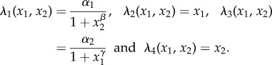
Table 5.

Circadian clock network: average speed-up factors of PPA with respect to other methods.

p	Girsanov	CFD	CRP
0.95	355.08	12.76	15.73
0.99	189.82	13.44	15.78

In the above expressions, x₁ and x₂ denote the number of molecules of and , respectively. We set α₁ = 50, α₂ = 16, β = 2.5 and γ = 1. Let (X(t))_t≥0 be the CTMC representing the dynamics with initial state (X₁(0), X₂(0)) = (0, 0). For T = 10 and f(x) = x₁, our goal is to estimate

for θ = α₁, α₂, β and γ. In other words, we would like to measure the sensitivity of the mean of the number of molecules at time T = 10, with respect to all the model parameters.

As the propensity functions λ₁ and λ₃ are nonlinear, it is difficult to compute S_θ(f, T) exactly. As before, we obtain close approximations of S_θ(f, T) using PPA (values given in the electronic supplementary material, §3), and then use these values in computing confidence levels of estimates. The CPU times needed by all the methods for two threshold confidence levels (p = 0.95 and p = 0.99) are presented in figure 5. As in the previous two examples, both CFD and CRP yield an estimate with the desired confidence level with h = 0.1 in all the cases.

Figure 5.

Efficiency comparison for genetic toggle switch with two threshold confidence levels: p = 0.95 (a) and p = 0.99 (b) and observation time T = 10. For finite-difference schemes, h = 0.1 was used in all the cases.

From figure 5, it can be easily seen that PPA is the best-performing method. The average speed-up factors for PPA with respect to other methods are given in table 6. They are calculated by aggregating CPU times for the four values of θ. Note that in this example, the unbiased schemes perform much better than the finite-difference schemes, possibly due to nonlinear parameter-dependence of the propensity functions.

Table 6.

Genetic toggle switch: average speed-up factors of PPA with respect to other methods.

p	Girsanov	CFD	CRP
0.95	7.57	7.81	21.34
0.99	7.62	10.11	45.02

The above examples illustrate that in producing an estimate with a specified statistical accuracy, PPA can be much more efficient than other methods, both biased and unbiased. The finite-difference schemes may outperform PPA in some cases but they can also be much slower in other cases. As it is difficult to independently verify the statistical accuracy of finite-difference schemes, PPA is an attractive alternative to these schemes, as its unbiasedness presents a theoretical guarantee for statistical accuracy.

5. Conclusion and future work

We provide a new unbiased method for estimating parameter sensitivity of stochastic reaction networks. Using a result from our recent paper [15], we construct a random variable whose expectation is the required sensitivity value. We then present a simple procedure, called the PPA, to compute the realizations of this random variable. This gives us a way to generate samples for estimating the parameter sensitivity. Our method can be viewed as an improved version of the APA, that we presented in [15]. Unlike APA, the proposed method is easy to implement, has low memory requirements and it works well for large networks and large observation times.

Through examples, we compare the performance of PPA with other methods for sensitivity estimation, both biased and unbiased. Our results indicate that PPA easily outperforms the unbiased Girsanov method. Moreover in many cases, it can even be faster than the best-performing finite-difference schemes (CRP and CFD) in producing a statistically accurate estimate. This makes PPA an appealing method for sensitivity estimation because it is computationally efficient and one does not have to tolerate a bias of an unknown size that is introduced by finite-difference approximations.

In our method, we simulate the paths of the underlying Markov process using Gillespie's SSA [16]. However, SSA is very meticulous in the sense that it simulates the occurrence of each and every reaction in the dynamics. This can be very cumbersome for large networks with many reactions. To resolve this problem, a class of τ-leaping methods have been developed [23,24]. These methods are approximate in nature, but they significantly reduce the computational effort that is required to simulate the reaction dynamics. In future, we would like to develop a version of PPA that uses a τ-leaping method instead of SSA and still produces an accurate estimate for the sensitivity values. Such a method would greatly simplify the sensitivity analysis of large networks. Recently, hybrid approaches that combine several existing sensitivity estimation methods in a multi-level setting have been introduced in [25]. Integrating PPA into this hybrid framework may further enhance its efficiency. This will be investigated in a future work.

Funding statement

We acknowledge funding from Human Frontier Science Programme (RGP0061/2011).

References

- 1.Érdi P, Tóth J. 1989. Mathematical models of chemical reactions. Nonlinear science: theory and applications. Theory and applications of deterministic and stochastic models. Princeton, NJ: Princeton University Press. [Google Scholar]
- 2.Thattai M, van Oudenaarden A. 2001. Intrinsic noise in gene regulatory networks. Proc. Natl Acad. Sci. USA 98, 8614–8619. ( 10.1073/pnas.151588598) [DOI] [PMC free article] [PubMed] [Google Scholar]
- 3.Hethcote H. 2000. The mathematics of infectious diseases. SIAM Rev. 42, 599–653. ( 10.1137/S0036144500371907) [DOI] [Google Scholar]
- 4.Bascompte J. 2010. Structure and dynamics of ecological networks. Science 329, 765–766. ( 10.1126/science.1194255) [DOI] [PubMed] [Google Scholar]
- 5.Berger SI, Iyengar R. 2009. Network analyses in systems pharmacology. Bioinformatics 25, 2466–2472. ( 10.1093/bioinformatics/btp465) [DOI] [PMC free article] [PubMed] [Google Scholar]
- 6.Elowitz MB, Levine AJ, Siggia ED, Swain PS. 2002. Stochastic gene expression in a single cell. Science 297, 1183–1186. ( 10.1126/science.1070919) [DOI] [PubMed] [Google Scholar]
- 7.McAdams H, Arkin A. 1997. Stochastic mechanisms in gene expression. Proc. Natl Acad. Sci. USA 94, 814–819. ( 10.1073/pnas.94.3.814) [DOI] [PMC free article] [PubMed] [Google Scholar]
- 8.Stelling J, Gilles ED, Doyle FJ. 2004. Robustness properties of circadian clock architectures. Proc. Natl Acad. Sci. USA 101, 13 210–13 215. ( 10.1073/pnas.0401463101) [DOI] [PMC free article] [PubMed] [Google Scholar]
- 9.Feng XJ, Hooshangi S, Chen D, Li R, Genyuan W, Rabitz H. 2004. Optimizing genetic circuits by global sensitivity analysis. Biophys. J. 87, 2195–2202. ( 10.1529/biophysj.104.044131) [DOI] [PMC free article] [PubMed] [Google Scholar]
- 10.Gunawan R, Cao Y, Doyle FJ. 2005. Sensitivity analysis of discrete stochastic systems. Biophys. J. 88, 2530–2540. ( 10.1529/biophysj.104.053405) [DOI] [PMC free article] [PubMed] [Google Scholar]
- 11.Rathinam M, Sheppard PW, Khammash M. 2010. Efficient computation of parameter sensitivities of discrete stochastic chemical reaction networks. J. Chem. Phys. 132, 034103 ( 10.1063/1.3280166) [DOI] [PMC free article] [PubMed] [Google Scholar]
- 12.Sheppard PW, Rathinam M, Khammash M. 2012. A pathwise derivative approach to the computation of parameter sensitivities in discrete stochastic chemical systems. J. Chem. Phys. 136, 034115 ( 10.1063/1.3677230) [DOI] [PMC free article] [PubMed] [Google Scholar]
- 13.Anderson D. 2012. An efficient finite difference method for parameter sensitivities of continuous time Markov chains. SIAM J. Numer. Anal. 50, 2237–2258. ( 10.1137/110849079) [DOI] [Google Scholar]
- 14.Plyasunov S, Arkin AP. 2007. Efficient stochastic sensitivity analysis of discrete event systems. J. Comput. Phys. 221, 724–738. ( 10.1016/j.jcp.2006.06.047) [DOI] [Google Scholar]
- 15.Gupta A, Khammash M. 2013. Unbiased estimation of parameter sensitivities for stochastic chemical reaction networks. SIAM J. Sci. Comput. 35, A2598–A2620. ( 10.1137/120898747) [DOI] [Google Scholar]
- 16.Gillespie DT. 1977. Exact stochastic simulation of coupled chemical reactions. J. Phys. Chem. 81, 2340–2361. ( 10.1021/j100540a008) [DOI] [Google Scholar]
- 17.Gibson MA, Bruck J. 2000. Efficient exact stochastic simulation of chemical systems with many species and many channels. J. Phys. Chem. A 104, 1876–1889. ( 10.1021/jp993732q) [DOI] [Google Scholar]
- 18.Glynn PW. 1990. Likelihood ratio gradient estimation for stochastic systems. Commun. ACM 33, 75–84. ( 10.1145/84537.84552) [DOI] [Google Scholar]
- 19.Ethier SN, Kurtz TG. 1986. Markov processes: characterization and convergence. Wiley Series in Probability and Mathematical Statistics, vol. 44. New York, NY: John Wiley. [Google Scholar]
- 20.Goutsias J. 2007. Classical versus stochastic kinetics modeling of biochemical reaction systems. Biophys. J. 92, 2350–2365. ( 10.1529/biophysj.106.093781) [DOI] [PMC free article] [PubMed] [Google Scholar]
- 21.Vilar JMG, Kueh HY, Barkai N, Leibler S. 2002. Mechanisms of noise-resistance in genetic oscillator. Proc. Natl Acad. Sci. USA 99, 5988–5992. ( 10.1073/pnas.092133899) [DOI] [PMC free article] [PubMed] [Google Scholar]
- 22.Gardner TS, Cantor CR, Collins JJ. 2000. Construction of a genetic toggle switch in Escherichia coli. Nature 403, 339–342. ( 10.1038/35002131) [DOI] [PubMed] [Google Scholar]
- 23.Gillespie DT. 2001. Approximate accelerated stochastic simulation of chemically reacting systems. J. Chem. Phys. 115, 1716–1733. ( 10.1063/1.1378322) [DOI] [Google Scholar]
- 24.Cao Y, Gillespie DT, Petzold LR. 2006. Efficient step size selection for the tau-leaping simulation method. J. Chem. Phys. 124, 044109 ( 10.1063/1.2159468) [DOI] [PubMed] [Google Scholar]
- 25.Wolf E, Anderson D. 2014. Hybrid pathwise sensitivity methods for discrete stochastic models of chemical reaction systems. (http://arxiv.org/abs/14083655) [DOI] [PubMed]