Learning regulatory programs by threshold SVD regression

Significance

With the increase in high-throughput data in genomic studies, the study of regulatory relationships between multidimensional predictors and responses is becoming a common task. Although high-dimensional data hold promise for revealing rich and complex regulations, it remains challenging to infer the relations between tens of thousands of responses and thousands of predictors, as the desired signal must be searched among an overwhelming number of irrelevant responses. Here we show that by formulating the regulatory programs as hidden-intermediate nodes in a linear network, a sparsity-inducing modeling and inference approach is effective in extracting the regulatory relations among very high-dimensional responses and predictors, even when the sample size is much lower.

Abstract

We formulate a statistical model for the regulation of global gene expression by multiple regulatory programs and propose a thresholding singular value decomposition (T-SVD) regression method for learning such a model from data. Extensive simulations demonstrate that this method offers improved computational speed and higher sensitivity and specificity over competing approaches. The method is used to analyze microRNA (miRNA) and long noncoding RNA (lncRNA) data from The Cancer Genome Atlas (TCGA) consortium. The analysis yields previously unidentified insights into the combinatorial regulation of gene expression by noncoding RNAs, as well as findings that are supported by evidence from the literature.

The development of microarray and next-generation sequencing technologies has enabled rapid quantification of various genome-wide features (DNA sequences, gene expressions, noncoding RNA expressions, methylation, etc.) in a population of samples (1, 2). Large consortia have compiled genetic and molecular profiling data in an enormous number of tumors across hundreds of samples (3, 4). A common challenge arising from these large-scale genomic studies is the inference of regulatory relationships between different genome-wide measurements from the complex biological systems where the number of predictors and responses often far exceeds the sample size.

To formulate a statistical model for such regulatory relations, consider the situation depicted in Fig. 1 (see Fig. S1 for more detailed illustration of the model schema), where $p$ regulators $\mathit{x}=(x_1,\dots ,x_p)$ regulate $q$ responses $\mathit{y}=(y_1,\dots ,y_q)$ through $r$ regulatory programs that are represented by hidden nodes, e.g., $h_1,\dots ,h_r$. The activity $h_j$ of the $j\text{th}$ program depends on the regulators connected to hidden node $j$, and $h_j$ in turn affects the level of the responses that are connected to node $j$. To express this model mathematically, we denote by ${\mathit{u}}_j$ and ${\mathit{v}}_j$ the unit vectors corresponding respectively to the input weights $\{a_{ij}$, $i=1,\dots ,p\}$ and the output weights $\{b_{jk}$, $k=1,\dots ,q\}$ of the $j\text{th}$ program. Then the regulatory relations are represented as $h_{\mathit{j}}=\sigma \left(\mathit{x}{\mathit{u}}_j\right)$ and $\mathit{y}={\displaystyle {\sum }_{j=1}^r{d}_j{h}_j{\mathit{v}\prime }_j}$, where $\mathit{x}$, $\mathit{y}$ are regarded as row vectors, $\mathit{u}$, $\mathit{v}$ are regarded as column vectors, and $\sigma$() is a sigmoidal function. The aforementioned is a standard single-layer neural network model that is widely used in predictive modeling but could be impossible to learn in biological studies where sample size $n$ is much smaller than $p$ or $q$. Thus, we first simplify the model by taking $\sigma$ to be the identity function. Then our model becomes $h_{\mathit{j}}=\mathit{x}{\mathit{u}}_j$, $\mathit{y}={\displaystyle {\sum }_{j=1}^r{d}_j{h}_j{\mathit{v}\prime }_j}$.

Fig. 1.

Schematic representation of the combinatorial regulation using regulatory programs. Circles represent $p$ predictors X, hexagons represent $q$ responses Y, and diamonds represent $r$ regulatory programs h. Predictors and responses were color matched to their corresponding related hidden programs. Each $a_{ij}$ represents the strength of the input from regulator $i$ to program $j$, where $i=1\dots p$ and $j=1\dots r$. Each $b_{jk}$ represents the strength of the input from program $j$ to output response $k$, where $j=1\dots r$ and $k=1\dots q$. The arrow indicates the direction of the input.

We make the biologically plausible assumption that only a small subset of regulators is contributing to any program and that each program regulates only a small subset of responses. Under this assumption, ${\mathit{u}}_j$ and ${\mathit{v}}_j$ are sparse vectors in ${\mathrm{ℝ}}^p$ and ${\mathrm{ℝ}}^q$, respectively. The magnitude of the output weight vector (denoted by $d_j$) represents the “importance” of the $j\text{th}$ program relative to other programs. Finally, the different programs are assumed to operate independently. Although there are many possible ways to enforce this independence, we choose to assume that ${\mathit{u}}_1,\dots ,{\mathit{u}}_r$ are orthogonal to each other and ${\mathit{v}}_1,\dots ,{\mathit{v}}_r$ are orthogonal to each other. This assumption enables us to develop fast algorithms for statistical inference of the model from observed data on $\mathit{y}$ and $\mathit{x}$.

It follows from the above assumptions that the ${\mathit{u}}_j$ s and ${\mathit{v}}_j$ s are respectively the left and right singular vectors in the singular value decomposition (SVD) of the coefficients matrix in the regression of $\mathit{y}$ on $\mathit{x}$. Although there have been considerable recent works on the use of sparse SVD in statistical modeling, most of them are targeted to the situation where only $\mathit{y}$ is observed and there is no predictor variable $\mathit{x}$ (5). An exception is reduced-rank stochastic regression with SVD (RRRR) (6), which to our knowledge seems to be the first to introduce a sparse SVD model for the regression relation. However, as will be seen below, our algorithm thresholding SVD (T-SVD) for learning the model is entirely new and provides substantial improvement in estimation accuracy as well as learning speed. Thus, besides making a conceptual contribution of formulating the regulatory programs as components in a sparse SVD model, our work also represents an advance in the statistical methodology for estimating such a model.

We demonstrate the better performance of our method compared with other existing methods using simulation data mimicking the sparse and combinatorial feature of complex biological systems. We also investigate the microRNA (miRNA)–gene regulation (i.e., regulation of gene expression by miRNA) and long noncoding RNA (lncRNA)–gene regulations by applying T-SVD to analyze a large ovarian cancer gene expression dataset from The Cancer Genome Atlas (TCGA) consortium (3). This analysis is challenging in that the sample size is substantially smaller than the number of regulators and responses. Our analysis reveals regulatory programs that associate specific miRNA or lncRNAs to relevant cancer pathways. Many of the regulator–target relationships are supported by external evidence from the literature.

Results

T-SVD Regression.

The above model implies that if $\mathit{y}$ and $\mathit{x}$ are respectively the response and regulator vectors measured from a given sample, then we have the regression relationship $E\left(\mathit{y}|\mathit{x}\right)=\mathit{x}\left({{\displaystyle \sum }}^{}{d}_j{\mathit{u}}_j{\mathit{v}\prime }_j\right)$. In other words, the $p\times q$ matrix of regression coefficients has a SVD decomposition with singular values $d_j$ and corresponding left- and right-singular vectors ${\mathit{u}}_j$ and ${\mathit{v}}_j$ for $j=1,\dots ,r$.

When response data are available from $n$ samples, they are denoted by an $n\times q$ matrix $Y$ whose rows correspond to the sample responses. Similarly, the regulator profiles for the $n$ samples are represented by an $n\times p$ matrix $X$. Our model can then be expressed in matrix form as $E\left(Y|X\right)=XC$, where $C={\displaystyle {\sum }_{\left\{j=1,\dots ,r\right\}}{d}_j{\mathit{u}}_j{\mathit{v}\prime }_j}=UD{V}^{\prime }$, $U=\left[{\mathit{u}}_1,\dots ,{\mathit{u}}_r\right]$, $V=\left[{\mathit{v}}_1,\dots ,{\mathit{v}}_r\right]$, and $D$ is the $r\times r$ diagonal matrix with diagonal $d_1\ge \dots \ge d_r>0$.

To fit the model we propose an iterative method. Conditional on $U$($\text{or\hspace{0.17em}}V$), we estimate $VD$ $(\text{or}\hspace{0.17em}UD)$ by a thresholding-based regularized multivariate regression step (Materials and Methods, Eqs. 2 and 3), which gives an estimated matrix that is sparse but not orthogonal (i.e., not having orthogonal columns). To obtain an orthogonal estimate we developed a sparse orthogonal decomposition algorithm (SODA) (Materials and Methods). SODA, unlike the standard Gram–Schmidt process, does not destroy sparsity. We iterate between the estimates of $U$ and $V$ until reaching convergence (Fig. S1).

Two additional methodological innovations were incorporated into our T-SVD regression algorithm. First, the threshold parameter in the thresholding step is automatically determined by a Bayesian information criterion (BIC)-like criterion that is specifically derived for our model (Materials and Methods). Second, to achieve speed and scalability the algorithm exploits sparsity in its computation by precomputing and storing terms that are not changed by the iteration and by indexing the nonzero rows in the sparse large matrices so that only the calculation involving nonzero rows would be carried out. For more details on the algorithm, see Materials and Methods.

Compared with sequential extraction algorithm (SEA) and iterative exclusive extraction algorithm (IEEA) methods (6), our T-SVD method is an entirely different algorithm approach to estimate a sparse SVD for the regression relation. Whereas SEA and IEEA try to estimate the singular vector pairs (${\mathit{u}}_j,{\mathit{v}}_j$) sequentially, starting from the pair with the largest singular value, our approach iterates between the estimation of the $U$ matrix and estimation of the $V$ matrix.

Simulation Study.

We performed comprehensive simulations to assess the performance of T-SVD relative to four existing methods. Table 1 lists the four methods and their references. Besides SEA and IEEA, we also include two biclustering-based methods (SSVD and BCssvd) (5, 7) in the comparison. Details of the simulation settings are given in Materials and Methods. Here we focus on the case where $n=100$, $p=150$, $q=150$, and the signal-to-noise ratio $(\text{S}2\text{N}$) = 1. Fig. 2 gives the comparison results for the inference of three sparse matrices: coefficient matrix $C$, left singular vectors $U$, and right singular vectors $V$. The metrics for comparison are in terms of sensitivity, specificity, and sum of squares of errors (SSE). As shown in Fig. 2, T-SVD outperforms competing algorithms in almost all different scenarios considered here. The sensitivity of T-SVD is among the highest when the maximum correlation ($\rho$) among regulators is below 0.5 but starts to decrease afterward. On the other hand, T-SVD almost always gives the highest specificity by a large margin and it also achieves the lowest total estimation error in terms of SSE. The high specificity of T-SVD means that it produces the sparsest estimate among all algorithms. It is interesting to note that the biclustering-based methods have much lower specificity. Similar comparison results hold in other simulation settings (Figs. S2 and S3).

Table 1.

List of existing algorithms used in comparison with T-SVD in the simulation study

Name	Brief description of the algorithm
SEA	Sequential extraction algorithm using SVD
IEEA	Iterative extraction algorithm using SVD
SSVD	Biclustering method using sparse SVD
BCssvd	Biclustering method using sparse SVD

Fig. 2.

Evaluation of different algorithms through simulations. We compared the performance of T-SVD, SEA, IEEA, SSVD, and BCssvd for the estimation of three matrices $C$ (A), $U$ (B), and $V$ (C). The dimensions of the simulation results are $n=100$, $p=150$, $q=150$. Details of the simulation methods are in Materials and Methods. We varied the parameter ρ, which represents the strength of the correlation among all predictors, from 0 (no correlation) to 0.625 (high correlation). From Left to Right, the three panels in each row represent the performance based on three different statistics: sensitivity (percentage of true nonzeros identified by each method), specificity (percentage of identified nonzero items being true), and SSE (sum of squared errors).

Performance of the BIC.

The BIC is a criterion widely used in model selection but it does not apply directly in our setting where n is much smaller than q. We proposed a new BIC for our model (Materials and Methods) and tested it by simulations against the standard BIC that simply used the number of nonzero entries of singular vectors as the number of free parameters. The results are given in Table S1. It is seen that the new BIC achieves a 10- to 100-fold decrease of incorrectly identified zeros in the estimation of $C,U$, and $V$.

In terms of computational efficiency, the two biclustering methods (SSVD and BCssvd) were the fastest (Table S2) but at the expense of greatly increasing the misclassification and estimation errors. T-SVD, although on average 200 times slower than biclustering methods, is nonetheless 50-fold and 180-fold faster than SEA and IEEA methods.

Application to Ovarian Cancer Data.

We demonstrate the capability of T-SVD by applying it to the miRNA and protein-coding gene expression data from TCGA ovarian cancer data (3). We also obtain lncRNA expression from a recent study that uses a bioinformatics approach to infer lncRNA expression from array data (8). Instead of using the whole set of lncRNA, we focus on a subset of 4,297 lncRNAs that have significant association with ovarian cancer-related traits. The final dataset consists of 487 samples with measurements of all three RNA types (254 miRNAs with SD > 0.5, 11,864 protein-coding genes, and 4,297 lncRNAs).

The numbers of regulatory programs (i.e., rank of C) in the miRNA–gene regulation (n = 487, P = 254, q = 11,864) and lncRNA–gene regulation (n = 487, P = 4,297, q = 11,864) were estimated to be 28 and 22, respectively, using T-SVD. For the miRNA–gene regulation analysis, T-SVD selected one to eight miRNAs and 284–431 genes per program (Fig. 3A), resulting in on average around 100-fold reduction in number of predictors as well as 30-fold reduction in number of responses (Table S3). The estimated lncRNA–gene regulation also showed substantial sparsity in each program (Fig. S4 and Table S4). Additionally, the set of regulators and response genes in each program (i.e., regulators and genes with nonzero edge weights in the program) shows minimal overlaps across programs (Fig. 3B). These together demonstrate that the T-SVD has succeeded in extracting independent and sparse regulatory programs from the data.

Fig. 3.

miRNA–gene regulation program properties. (A) Distribution of the number of predictor miRNAs and response genes in each of the programs. (B) Venn diagram showing that there are minimal overlaps among different programs in $V$. (C) The expression heat map of predictor miRNAs and response genes on the first regulatory program. Columns correspond to samples and rows correspond to genes and miRNAs, and expression levels from low to high are coded in a blue to red color scheme. The samples are clustered using the expressions of the nonzero response genes on the first program, and there is clear clustering of immunoreactive and proliferative subtype samples based on the expression profile for this particular program.

miRNA–Gene Regulation.

A singular value d_i reflects the relative importance of the corresponding program. Thus, we would expect to see the first regulation program capture the global gene expression pattern within the samples. A previous study from TCGA (3) classified the 487 ovarian cancer samples into four subtypes (immunoreactive, differentiated, proliferative, and mesenchymal) based on the global gene expression profile. Little was known regarding which miRNAs might be more related to the gene expression cancer subtypes. Program 1 in the miRNA–gene regulation clearly captured the major subtypes, especially the immunoreactive and proliferative subtypes (Fig. 3C). The majority of genes and four of five miRNAs in this program show high expression in immunoreactive subtype samples and low expression in proliferative subtype samples. Interestingly, miR-142 was identified as the strongest signature associated with lymphocyte-specific gene expression and methylation across multiple cancer types in another study (9). Several recent cancer studies also supported the inhibitory effect on cell proliferation by miR-142-3p in pancreatic cancer (10) and miR-224 in ovarian cancer (11). The only miRNA that showed high expression in proliferative subtype and low expression in immunoreactive subtype is miR-218. However, recent studies suggested its role as a tumor suppressor and inhibiting cell proliferation (12, 13). This suggested the complexities of miRNA regulations in different cancer types. High-throughput experimental approaches such as CLIP-SEq (14) in the ovarian cancer-related cells would help to elucidate the direct targets and functional roles of these miRNAs.

The response genes from the top programs showed enrichment in cancer-related KEGG and Reactome pathways, including pathways in cancer, transcriptional misregulation in cancer, cell adhesion, and GPCR signaling pathways (15) (Fig. S5). Based on information in a recent review paper (16), the vast majority (10 of 14) of the miRNAs from the top three programs were related to cancer. We use program 3 as an example, to illustrate the ability of T-SVD to capture important miRNA–gene regulation pathways. As shown in Fig. 4A, the response genes in this program are strongly enriched in cell adhesion and virus infection-related pathways. The results are also compared with information from starBase, a database of miRNA–target interaction constructed from combined evidence of sequence-based predictions and 14 large-scale RNA–protein interaction experimental datasets (17). We used starBase entries supported by at least one RNA–protein interaction experiment as the true interaction reference. In general only 1.9% of miRNA–gene pairs have support from starBase, whereas we found that 3.8% of the miRNA–gene pairs on this program have support from starBase, which represents a twofold enrichment and is strongly significant (hypergeometric P value = 4e-7, Fig. 4B).

Fig. 4.

Functional analysis of program 3 of miRNA–gene regulations. (A) Significantly enriched KEGG pathways. (B) Pie charts showing the miRNA–gene regulations predicted by T-SVD are significantly enriched by experimental supports based on starBase. (C) Network of experimentally validated miRNA–gene interactions for the ECM–receptor interaction pathway. Only target genes based on the experimentally validated database starBase are shown. Genes are shown as circles and miRNAs are shown as boxes.

In particular, 6 of the 11 genes in the enriched ECM–receptor interaction pathway showed evidence of interaction with multiple miRNAs identified as regulators in program 3 (Fig. 4C). Both let-7 and miR-29b were demonstrated to play critical roles in cancer proliferation and the ECM pathway in other cancer types (18, 19). Furthermore, the main target gene of let-7 in lung cancer (18), HMGA2, was recently shown to induce ovarian surface epithelial transformation through regulation of EMT genes (20). Taken together, these results suggest that let-7, miR-29b, and perhaps some of the other miRNAs in program 3 may play regulatory roles in ovarian cancer through extracellular matrix pathways.

lncRNA–Gene Regulation.

Because knowledge of lncRNA targets and functions is limited, we focused on the enriched Gene Ontology (GO) (21) categories of the response genes in top programs from T-SVD. The enriched GO categories in the top three programs include cell cycle, chromatin organization, chromatin modification, and mitochondrion, etc. (Fig. S6).

Many well-studied lncRNAs [e.g., Xist (22), HOTAIR (23), and HOTTIP (24)] regulate gene expression through interactions with chromatin modification complexes and then targeting these enzymatic activities to appropriate locations in the genome (25). Programs 2 and 3 are significantly associated in chromatin regulation-related GO categories (Fig. S6). Eighty-eight genes in the chromatin modification (chromatin regulation, CR) biological process (GO:0016568) are found in the response genes in program 2 (hypergeometric test P value = 6.8e-7). There are 2 CR genes CENPN and CCNB1 among the top 20 genes in this program if we rank genes by the magnitude of the corresponding component of the left singular vector of the program. CENPN was recently identified as a core component in a breast cancer prognostic gene signature (26).

Because many lncRNAs are involved in cis-regulation (27), we examined whether the high-ranking genes are near the same genomic locus of the regulatory lncRNAs in a program. One of the strongest lncRNAs in program 2, ENSG00000233589 (RP4-694A7.2), was found to be on the antisense strand of gene DEPDC1. The coefficient estimate from T-SVD (shown below the diagonal line in Fig. 5) was very strong as corroborated by the pairwise Pearson correlation coefficient (r = 0.6, shown above the diagonal line in Fig. 5). An additional program that showed CR gene enrichment is program 13, which has HMGA2 as a top-ranking response gene (Fig. S7). HMGA2 is the main target gene of let-7 mirRNA in lung cancer (18) and also found to be strongly regulated by miRNA let-7c in our miRNA–gene regulation analysis. Finally we note that although the above analysis shows that some of the top lncRNA–gene regulations have substantial support from the literature, the exact molecular mechanism of these lncRNAs and their direct targets needs further experimental evaluation.

Fig. 5.

Coefficient estimate and pairwise Pearson correlation of the lncRNA–gene regulation matrix in program 2. Coefficient estimates from the T-SVD (color and dot size rescaled to [−1, 1]) are shown in the lower left triangle below the diagonal line and pairwise Pearson correlation coefficients are plotted in the upper right triangle. Only the top 20 (in absolute C value) genes in program 2 are listed. Gene names are colored red for CR (chromatin regulator) genes. Neighboring genes of significant lncRNAs are marked with an asterisk after the name. Note that the pairwise correlations can be either negative or positive, although they are all positive in the subset of the top 20 genes in this particular program.

Discussion

SVD has previously been used in biclustering of genes and samples based on a sample of gene expression profiles (5, 28). The use of sparse SVD to model the regression relation (i.e., the matrix C) was first introduced in the RRRR method. However, RRRR is not guaranteed to give orthogonal singular vectors and its approach of sequential extraction of rank one components does not scale well to a high dimension. This is confirmed in our simulations. Another joint variable and rank selection method (29) uses $l_2$ group penalty on the rows of $C$. However, this algorithm along with another recently proposed method (30) can reduce dimension in predictor space but not response space and does not provide information on independent regulatory programs. A sparse network-regularized multiple nonnegative matrix factorization (SNMNMF), which incorporates the known interaction from literature as a prior information in the parameter estimations, was recently proposed for the inference of miRNA–gene regulation (31). However, SNMNMF identifies only the coexistence relationship between predictors and responses without the estimation of the relative strength or direction of regulation.

Here, we formally established connections between the regulation networks and SVD regression both conceptually and mathematically and proposed an SVD regression-based model (T-SVD) for learning regulatory programs in a complex biological system. Our model can capture the association between a large number of predictors and responses simultaneously and identify regulatory relationships between subsets of regulators and subsets of responses. The learning of independent regulatory programs provides deeper insight into the complex regulatory relations underlying the biological system.

Other than the ncRNA–gene regulation examples shown here, the T-SVD framework is applicable to other areas of genomic studies such as the inference of shared trans-expression QTL and global regulation of epigenetic markers on gene expression, etc. We have implemented the T-SVD method as a freely available R package named “T_SVD”.

Materials and Methods

T-SVD Model.

With the SVD representation of the coefficient matrix, model $Y=XC+E$ becomes

$$Y=XUD{V}^{\prime }+E.$$ [1]

The SVD expression of $C$ represents $r$ programs of parameters with decreasing importance and each program relates the responses to the predictors in a unique way. For the $k\text{th}$ program, ${\mathit{u}}_k$ is interpreted as the predictor effect, ${\mathit{v}}_k$ is interpreted as the response effect, and $d_k$ indicates the relative importance of the program. When ${\mathit{u}}_k$ and ${\mathit{v}}_k$ are sparse with many zero entries, only a few predictors can be accounted for the effect of the $k\text{th}$ program with only a few responses being predicted.

We propose to estimate $U$ and $V$ by an iterative thresholding algorithm similar to the one used in Yang et al. (7) for sparse SVD decomposition of a matrix. To be more specific, first fix $U$. Let $X_v=XU$ and $V_v=VD$. Then

$$Y=X_v{V\prime }_v+E.$$ [2]

Here $V_v$ is a matrix with sparse and orthogonal columns. Because $r<p$, we estimate $V_v$ initially by ${\widehat{V}}_v={\left\{{\left({X\prime }_v{X}_v\right)}^{-1}{X\prime }_{v}Y\right\}}^{\prime }$. To “kill” the small coordinates in ${\widehat{V}}_v$, we threshold ${\widehat{V}}_v$ with a thresholding function ${\Theta }_v$ so that ${\widehat{V}}_v^{\text{thr}}={\Theta }_v\left({\widehat{V}}_v\text{;}{\gamma }_v\right)$. Although the Gram–Schmidt process can be used to extract the orthogonal component for ${\widehat{V}}_v^{\text{thr}}$, it is not guaranteed to produce a sparse result even if ${\widehat{V}}_v^{\text{thr}}$ itself is sparse. Consequently we develop a novel SODA to ${\widehat{V}}_v^{\text{thr}}$ and obtain an estimate with sparse and orthogonal columns. SODA is similar to the QR decomposition but is more appropriate for extracting sparse orthogonal vectors; details are provided later. Next fix $V$. Multiplying Eq. 1 from the right by $V$ leads to

$$Y_u=X{U}_u+E_u,$$ [3]

where $Y_u=YV$, $U_u=UD$, and $E_u=EV$. Here $U_u$ is also a matrix containing sparse and orthogonal columns. If $p\le n$, we can estimate $U_u$ similarly as before. We focus on the case $p>n$, where regularization methods are needed. We adopt the thresholding-based iterative procedure (32), which iterates

$$U_u^{\left(k\right)}={\Theta }_u\left\{\left(I_p-\frac{\Sigma }{{\Vert \Sigma \Vert }_2}\right)U_u^{\left(k-1\right)}+\frac{X^{\prime }Y{V}^k}{{\Vert \Sigma \Vert }_2}\text{;}\hspace{0.5em}{\gamma }_u\right\}.$$ [4]

Here $\Sigma =X^{\prime }X$, ${\Vert \Sigma \Vert }_2$ is the operator norm of $\Sigma$, ${\Theta }_u$ is a thresholding function, and ${\gamma }_u$ is a thresholding parameter. Because we iterate between the estimates of $U$ and $V$, we can just iterate [4] once. Then we apply SODA again to obtain an estimate of $U$.

The proposed iterative thresholding algorithm is named T-SVD and is shown below.

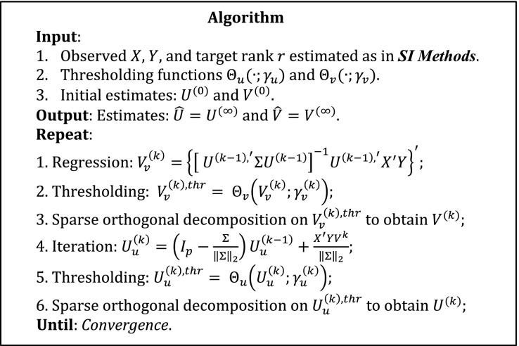
The superscript $\left(k\right)$ indicates the $k$ th iteration. The detailed information on the thresholding function is given in SI Materials and Methods. The algorithm reduces to the algorithm in ref. 7 if $X$ is an identity matrix, except that we use the sparse orthogonal decomposition instead of the usual QR decomposition in steps 3 and 5.

Further Details for Estimation.

Sparse orthogonal decomposition.

The sparse orthogonal decomposition is designed to extract sparse and orthogonal eigenvectors from a sparse matrix. To illustrate the idea, we consider a two-column matrix $[{\mathit{u}}_1$, ${\mathit{u}}_2]$. The QR decomposition gives an orthogonal matrix $[{\mathit{v}}_1$, ${\mathit{v}}_2]$, where ${\mathit{v}}_1={\mathit{u}}_1/\Vert {\mathit{u}}_1\Vert$ and ${\mathit{v}}_2={\tilde{\mathit{v}}}_2/\Vert {\tilde{\mathit{v}}}_2\Vert$ with ${\tilde{\mathit{v}}}_2={\mathit{u}}_2-\left({{\mathit{u}}^{\prime }}_2{\mathit{v}}_1\right){\mathit{v}}_1$. Suppose ${\mathit{u}}_1$ and ${\mathit{u}}_2$ are both sparse; then ${\mathit{v}}_2$ might contain more nonzero entries than ${\mathit{u}}_2$ because of the orthogonal constraint with ${\mathit{u}}_1$. The sparse orthogonal decomposition changes only the nonzero entries of ${\mathit{u}}_2$ so that the entries in ${\mathit{v}}_2$ remain zero whenever the corresponding entries in ${\mathit{u}}_2$ are zero. Let $\left[{\mathit{v}}_1^{*},\hspace{0.17em}{\mathit{v}}_2^{*}\right]$ denote the resulting singular vectors from the sparse orthogonal decomposition. The following is an example:

$$\left[{\mathit{u}}_1\hspace{0.5em}{\mathit{u}}_2\right]=\left(\begin{array}{rr}\hfill 1& \hfill 0\\ \hfill 1& \hfill 0\\ \hfill 1& \hfill 1\\ \hfill 1& \hfill -0.9\end{array}\right)\text{;}\hspace{1em}\left[{\mathit{v}}_1\hspace{0.5em}{\mathit{v}}_2\right]=\left(\begin{array}{rr}\hfill 0.5& \hfill -0.019\\ \hfill 0.5& \hfill -0.019\\ \hfill 0.5& \hfill 0.725\\ \hfill 0.5& \hfill -0.688\end{array}\right)\text{;}\hspace{1em}\left[{\mathit{v}}_1^{\ast },\hspace{0.17em}{\mathit{v}}_2^{\ast }\right]=\left(\begin{array}{rr}\hfill 0.5& \hfill 0\\ \hfill 0.5& \hfill 0\\ \hfill 0.5& \hfill 0.707\\ \hfill 0.5& \hfill -0.707\end{array}\right).$$

Therefore, the sparse orthogonal decomposition may provide more sparse orthogonal vectors than the QR decomposition. The sparse orthogonal decomposition has some limitation. It will fail algebraically if the third entry of ${\mathit{u}}_2$ is zero. In such a case, we revert back to the QR decomposition.

Initialization and implementation.

The proposed algorithm requires an initial estimate, $U^{\left(0\right)}$, $V^{\left(0\right)}$, and $d^{\left(0\right)}$, which can be obtained from an initial estimate of $C$ through the SVD. One plausible estimator is the reduced-rank least squares estimator (33, 34), which is consistent for high-dimensional data (35). Another one is the ridge regression estimator in which a small identity matrix $\epsilon I_p$ is added to $\Sigma$ to make it invertible. In the simulation study and for the real data, we use the ridge estimator and let $\epsilon =\left(0.1/p\right){\displaystyle {\sum }_{i=1}^n{\lambda }_i(\Sigma )}$, where ${\lambda }_i(\Sigma )$ is the $i$ th singular value of $\Sigma$.

The accuracy of the algorithm may depend on the initial estimate. To reduce the effect of the initial estimate, we adopt a two-step procedure. We first run the proposed algorithm with the ridge estimator as starting values, and then we use the resulting estimate as a new initial estimator and run the algorithm again and obtain the final estimate.

Selection of the tuning parameters.

Our idea is to combine the BICs for conditional models and propose the criterion $\text{BIC}=\log \left(\text{SSE}\right)+\left(\log \left(rn\right)/rn\right){\text{df}}_v+\left(\log \left(qn\right)/qn\right){\text{df}}_u$, where $\mathrm{SSE}={\Vert Y-X\widehat{U}\widehat{D}{\widehat{V}}^{\prime }\Vert }_F^2$, ${\text{df}}_v$ is the degrees of freedom of model [2], and ${\text{df}}_u$ is the degrees of freedom of model [3]. Here ${\Vert \cdot \Vert }_F$ is the Frobenius norm. Conditional on $U$, our estimation procedure with a hard-thresholding function is equivalent to an $l_0$ penalization (31), and hence without the orthogonal constraints, the number of nonzero entries in the final estimate of ${\widehat{V}}_v$ can be easily shown to be an unbiased estimator of the degrees of freedom of the $l_0$ penalization. Therefore, we estimate ${\text{df}}_v$ by $\widehat{{\text{df}}_v}=\#\left(\widehat{V}!=0\right)-r\left(r-1\right)/2$, where $\#(\cdot )$ denotes the number of true statements in a vector of expressions or in a matrix of expressions. Note that we subtract $r\left(r-1\right)/2$ in the above formula as there are $r\left(r-1\right)/2+r$ constraints in $\widehat{V}$ and $r$ free parameters in $\widehat{D}$. Conditional on $V$, the number of nonzero elements in the final estimate of ${\widehat{U}}_u$ underestimates the degrees of freedom of the hard-thresholded least-squares estimation; however, the bias is negligible under some mild conditions. Therefore, we estimate ${\text{df}}_u$ by $\widehat{{\text{df}}_u}=\#\left(\widehat{U}!=0\right)-r\left(r-1\right)/2$. The derivation of the degrees of freedom of the hard-thresholded least-squares estimation is given in SI Materials and Methods.

Simulation.

The rank of the coefficient matrix was fixed at 3. The design matrix $X$, of size $n\times p$, is generated from a multivariate normal distribution with mean $0$ and covariance matrix $\Sigma$ where the $(k,j)$ th entry of Σ is defined as ${\Sigma }_{kj}={\rho }^{\left|k-j\right|}$ for $k=1\dots n\text{;}\hspace{0.17em}j=\hspace{0.17em}1\dots p$. Here $\rho$, which represents the strength of the correlation among all predictors, either is $0$ for the independent case or varies from 0.125 to 0.625 with an increment of 0.125 for the dependent case. Let $C=UD{V}^{\prime }$, where $U\hspace{0.17em}\text{and}\hspace{0.5em}V$, whose unnormalized values are shown in Table S5, be three-column orthogonal matrices containing left and right singular vectors, respectively. $D$ is a $3\times 3$ diagonal matrix with diagonal entries of (20, 10, 5). The response matrix $Y$ is generated by $Y=XC+E$, where $E$ is the matrix with i.i.d. errors from $\mathcal{N}(0,{\sigma }^2)$. We varied ${\sigma }^2$ to achieve different levels of S2Ns; i.e., ${\sigma }^2=\left\{{\displaystyle \sum }\text{diag}(C^{\prime }\times \Sigma \times C)\right\}/(n\times q\times s2r)$. For each scenario, 200 replications were simulated. Two algorithms, SEA and IEEA from the reduced-rank stochastic regression model (6) implemented in the R package “RRRR,” were included in the comparison. Two SVD biclustering models SSVD and BCssvd (5, 7) implemented in R Packages “ssvd” and “s4vd” were also included in the comparison. Because SSVD and BCssvd are biclustering algorithms, the input matrix was calculated by ${\left(X^{\prime }X\right)}^{-1}{X}^{\prime }Y$ for $n>p$ and ${(X^{\prime }X+0.1\times \min \left(d\right)/p\times \text{diag}\left(p\right))}^{-1}{X}^{\prime }Y$ for $n\le p$, and $d$ is the vector of singular values of $X$. All algorithms were assessed for sensitivity (percentage of true nonzeros identified by each method) and specificity (percentage of identified nonzero items being true), as well as sum of squared errors, which is defined as $\text{SSE}\left(\widehat{\cdot },\cdot \right)={\Vert \widehat{\cdot }-\cdot \Vert }^2$ for $C$, $U$, and $V$, respectively. The average computation time for each algorithm was also recorded.

Ovarian Cancer TCGA Data.

The miRNA and gene expression data for the 489 published samples (487 samples have measurements in both miRNA and gene expression) were obtained from the TCGA ovarian cancer study (3) companion website: tcga-data.nci.nih.gov/docs/publications/ov2011/. Unified expression of 11,864 genes from three different platforms (Agilent, Affymetrix HuEx, and Affymetrix U133A) along with the 254 miRNAs with large variation (SD > 0.5) from the original data file were used to carry out the analysis. The lncRNA expression data were extracted from a recent study (8), and the predictors are selected to be the 4,297 lncRNAs including literature-curated lncRNAs, ovarian cancer subtype-specific lncRNAs, lncRNAs associated with overall or progression-free survival, and lncRNAs associated with local copy number changes.

Functional Pathways and GO Categories Enriched in Predicted Response Genes.

We used the Cytoscape plug-in ClueGO (36) for the functional analysis of the predicted response genes in the miRNA–gene and lncRNA–gene regulation. We obtained the significantly enriched (Benjamini–Hochberg corrected P value <0.05) KEGG and Reactome (37) pathways for the predicted response genes from T-SVD in each program. For the lncRNA–gene regulation, we also searched for the large (>50 overlapping genes) significantly enriched biological processes in GO. As previous lncRNA studies suggest the important role of lncRNA in chromatin regulation (25), we collected a CR-related gene list by assembling all genes associated to GO category chromatin modification (GO:0016568) and its offspring. Then we specifically tested the enrichment of CR genes for the predicted response genes in each program by hypergeometric test.

References

- 1.Brown PO, Botstein D. Exploring the new world of the genome with DNA microarrays. Nat Genet. 1999;21(1) Suppl:33–37. doi: 10.1038/4462. [DOI] [PubMed] [Google Scholar]
- 2.Mortazavi A, Williams BA, McCue K, Schaeffer L, Wold B. Mapping and quantifying mammalian transcriptomes by RNA-Seq. Nat Methods. 2008;5(7):621–628. doi: 10.1038/nmeth.1226. [DOI] [PubMed] [Google Scholar]
- 3.Cancer Genome Atlas Research Network Integrated genomic analyses of ovarian carcinoma. Nature. 2011;474(7353):609–615. doi: 10.1038/nature10166. [DOI] [PMC free article] [PubMed] [Google Scholar]
- 4.Barretina J, et al. The Cancer Cell Line Encyclopedia enables predictive modelling of anticancer drug sensitivity. Nature. 2012;483(7391):603–607. doi: 10.1038/nature11003. [DOI] [PMC free article] [PubMed] [Google Scholar]
- 5.Lee M, Shen H, Huang JZ, Marron JS. Biclustering via sparse singular value decomposition. Biometrics. 2010;66(4):1087–1095. doi: 10.1111/j.1541-0420.2010.01392.x. [DOI] [PubMed] [Google Scholar]
- 6.Chen K, Chan K-S, Stenseth NC. Reduced rank stochastic regression with a sparse singular value decomposition. J R Stat Soc B. 2012;74(2):203–221. [Google Scholar]
- 7.Yang D, Ma Z, Buja A. 2013. A sparse SVD method for high-dimensional data. J Comput Graph Stat arXiv:1112.2433v1.
- 8.Du Z, et al. Integrative genomic analyses reveal clinically relevant long noncoding RNAs in human cancer. Nat Struct Mol Biol. 2013;20(7):908–913. doi: 10.1038/nsmb.2591. [DOI] [PMC free article] [PubMed] [Google Scholar]
- 9.Andreopoulos B, Anastassiou D. Integrated analysis reveals hsa-miR-142 as a representative of a lymphocyte-specific gene expression and methylation signature. Cancer Inform. 2012;11:61–75. doi: 10.4137/CIN.S9037. [DOI] [PMC free article] [PubMed] [Google Scholar]
- 10.MacKenzie TN, et al. Triptolide induces the expression of miR-142-3p: A negative regulator of heat shock protein 70 and pancreatic cancer cell proliferation. Mol Cancer Ther. 2013;12(7):1266–1275. doi: 10.1158/1535-7163.MCT-12-1231. [DOI] [PMC free article] [PubMed] [Google Scholar]
- 11.White NM, et al. Three dysregulated miRNAs control kallikrein 10 expression and cell proliferation in ovarian cancer. Br J Cancer. 2010;102(8):1244–1253. doi: 10.1038/sj.bjc.6605634. [DOI] [PMC free article] [PubMed] [Google Scholar]
- 12.Uesugi A, et al. The tumor suppressive microRNA miR-218 targets the mTOR component Rictor and inhibits AKT phosphorylation in oral cancer. Cancer Res. 2011;71(17):5765–5778. doi: 10.1158/0008-5472.CAN-11-0368. [DOI] [PubMed] [Google Scholar]
- 13.Venkataraman S, et al. MicroRNA 218 acts as a tumor suppressor by targeting multiple cancer phenotype-associated genes in medulloblastoma. J Biol Chem. 2013;288(3):1918–1928. doi: 10.1074/jbc.M112.396762. [DOI] [PMC free article] [PubMed] [Google Scholar]
- 14.Zhang C, Darnell RB. Mapping in vivo protein-RNA interactions at single-nucleotide resolution from HITS-CLIP data. Nat Biotechnol. 2011;29(7):607–614. doi: 10.1038/nbt.1873. [DOI] [PMC free article] [PubMed] [Google Scholar]
- 15.Dorsam RT, Gutkind JS. G-protein-coupled receptors and cancer. Nat Rev Cancer. 2007;7(2):79–94. doi: 10.1038/nrc2069. [DOI] [PubMed] [Google Scholar]
- 16.Koturbash I, Zemp FJ, Pogribny I, Kovalchuk O. Small molecules with big effects: The role of the microRNAome in cancer and carcinogenesis. Mutat Res. 2011;722(2):94–105. doi: 10.1016/j.mrgentox.2010.05.006. [DOI] [PubMed] [Google Scholar]
- 17.Li JH, Liu S, Zhou H, Qu LH, Yang JH. starBase v2.0: Decoding miRNA-ceRNA, miRNA-ncRNA and protein-RNA interaction networks from large-scale CLIP-Seq data. Nucleic Acids Res. 2014;42(Database issue):D92–D97. doi: 10.1093/nar/gkt1248. [DOI] [PMC free article] [PubMed] [Google Scholar]
- 18.Mayr C, Hemann MT, Bartel DP. Disrupting the pairing between let-7 and Hmga2 enhances oncogenic transformation. Science. 2007;315(5818):1576–1579. doi: 10.1126/science.1137999. [DOI] [PMC free article] [PubMed] [Google Scholar]
- 19.Park SY, Lee JH, Ha M, Nam JW, Kim VN. miR-29 miRNAs activate p53 by targeting p85 alpha and CDC42. Nat Struct Mol Biol. 2009;16(1):23–29. doi: 10.1038/nsmb.1533. [DOI] [PubMed] [Google Scholar]
- 20.Wu J, et al. HMGA2 overexpression-induced ovarian surface epithelial transformation is mediated through regulation of EMT genes. Cancer Res. 2011;71(2):349–359. doi: 10.1158/0008-5472.CAN-10-2550. [DOI] [PMC free article] [PubMed] [Google Scholar]
- 21.Ashburner M, et al. The Gene Ontology Consortium Gene ontology: Tool for the unification of biology. Nat Genet. 2000;25(1):25–29. doi: 10.1038/75556. [DOI] [PMC free article] [PubMed] [Google Scholar]
- 22.Maenner S, et al. 2-D structure of the A region of Xist RNA and its implication for PRC2 association. PLoS Biol. 2010;8(1):e1000276. doi: 10.1371/journal.pbio.1000276. [DOI] [PMC free article] [PubMed] [Google Scholar]
- 23.Tsai MC, et al. Long noncoding RNA as modular scaffold of histone modification complexes. Science. 2010;329(5992):689–693. doi: 10.1126/science.1192002. [DOI] [PMC free article] [PubMed] [Google Scholar]
- 24.Wang KC, et al. A long noncoding RNA maintains active chromatin to coordinate homeotic gene expression. Nature. 2011;472(7341):120–124. doi: 10.1038/nature09819. [DOI] [PMC free article] [PubMed] [Google Scholar]
- 25.Rinn JL, Chang HY. Genome regulation by long noncoding RNAs. Annu Rev Biochem. 2012;81:145–166. doi: 10.1146/annurev-biochem-051410-092902. [DOI] [PMC free article] [PubMed] [Google Scholar]
- 26.Wu G, Stein L. A network module-based method for identifying cancer prognostic signatures. Genome Biol. 2012;13(12):R112. doi: 10.1186/gb-2012-13-12-r112. [DOI] [PMC free article] [PubMed] [Google Scholar]
- 27.Guil S, Esteller M. Cis-acting noncoding RNAs: Friends and foes. Nat Struct Mol Biol. 2012;19(11):1068–1075. doi: 10.1038/nsmb.2428. [DOI] [PubMed] [Google Scholar]
- 28.Alter O, Brown PO, Botstein D. Singular value decomposition for genome-wide expression data processing and modeling. Proc Natl Acad Sci USA. 2000;97(18):10101–10106. doi: 10.1073/pnas.97.18.10101. [DOI] [PMC free article] [PubMed] [Google Scholar]
- 29.Bunea F, She Y, Wegkamp MH. Joint variable and rank selection for parsimonious estimation of high-dimensional matrices. Ann Stat. 2012;40(5):2359–2388. [Google Scholar]
- 30.Ma Z, Sun T. 2014. Adaptive sparse reduced-rank regression. arXiv:1403.1922.
- 31.Zhang S, Li Q, Liu J, Zhou XJ. A novel computational framework for simultaneous integration of multiple types of genomic data to identify microRNA-gene regulatory modules. Bioinformatics. 2011;27(13):i401–i409. doi: 10.1093/bioinformatics/btr206. [DOI] [PMC free article] [PubMed] [Google Scholar]
- 32.She Y. Thresholding-based iterative selection procedures for model selection and shrinkage. Electron J Stat. 2009;3:384–415. [Google Scholar]
- 33.Anderson TW. Estimating linear restrictions on regression coefficients for multivariate normal distributions. Ann Math Stat. 1951;22(3):327–351. [Google Scholar]
- 34.Reinsel GC, Velu RP. Partially reduced-rank multivariate regression models. Stat Sin. 2006;16:899–917. [Google Scholar]
- 35.Bunea F, She Y, Wegkamp MH. Optimal selection of reduced rank estimators of high-dimensional matrices. Ann Stat. 2011;39(2):1282–1309. [Google Scholar]
- 36.Bindea G, et al. ClueGO: A Cytoscape plug-in to decipher functionally grouped gene ontology and pathway annotation networks. Bioinformatics. 2009;25(8):1091–1093. doi: 10.1093/bioinformatics/btp101. [DOI] [PMC free article] [PubMed] [Google Scholar]
- 37.Wu G, Feng X, Stein L. A human functional protein interaction network and its application to cancer data analysis. Genome Biol. 2010;11(5):R53. doi: 10.1186/gb-2010-11-5-r53. [DOI] [PMC free article] [PubMed] [Google Scholar]
Associated Data
This section collects any data citations, data availability statements, or supplementary materials included in this article.