DL-PRO: A Novel Deep Learning Method for Protein Model Quality Assessment

Abstract

Computational protein structure prediction is very important for many applications in bioinformatics. In the process of predicting protein structures, it is essential to accurately assess the quality of generated models. Although many single-model quality assessment (QA) methods have been developed, their accuracy is not high enough for most real applications. In this paper, a new approach based on C-α atoms distance matrix and machine learning methods is proposed for single-model QA and the identification of native-like models. Different from existing energy/scoring functions and consensus approaches, this new approach is purely geometry based. Furthermore, a novel algorithm based on deep learning techniques, called DL-Pro, is proposed. For a protein model, DL-Pro uses its distance matrix that contains pairwise distances between two residues’ C-α atoms in the model, which sometimes is also called contact map, as an orientation-independent representation. From training examples of distance matrices corresponding to good and bad models, DL-Pro learns a stacked autoencoder network as a classifier. In experiments on selected targets from the Critical Assessment of Structure Prediction (CASP) competition, DL-Pro obtained promising results, outperforming state-of-the-art energy/scoring functions, including OPUS-CA, DOPE, DFIRE, and RW.

I. INTRODUCTION

Knowledge of three-dimensional (3D) structure of a protein is critical for understanding its function, mutagenesis experiments and drug developments. Several experimental methods such as the X-ray crystallography or Nuclear Magnetic Resonance (NMR) can help determine a good 3D structure but they are very time-consuming and expensive [1]. To address those limitations, computational protein structure prediction methods have been developed, including Modeller [2], HHpred [3], I-TASSER [4], Robetta [5], and MUFOLD [6]. The process of predicting protein structure commonly involves generating a large number of models, from which good models are selected using some quality assessment method.

Although many protein model quality assessment (QA) methods have been developed, such as MUFOLD-WQA [7], QMEANClust [8] MULTICOM [9], OPUS_CA [10], RW [11], etc, they all have various limitations and are not applicable to real applications. The Critical Assessment of Structure Prediction (CASP) is a biennial world-wild event in the structure prediction community to assess the current protein modeling techniques, including QA methods. In CASPs, different prediction software programs from various research groups were given unknown proteins to predict their structures. State-of-the-art single-model quality assessment methods include various energy functions or scoring functions, such as OPUS_CA [10], DFIRE [12], RW [11], DOPE [13], etc. In CASP competitions [14,15], the accuracy of single-model QA methods has been improving consistently, but still not very high in most cases. In contrast, consensus QA methods, such as MUFOLD-WQA and United3D, which are based on structure similarity, performed well on QA tasks, much better than single-model QA methods [14, 15]. The drawback of consensus QA methods is that they require a pool of diverse models to work well, which is not always available. More importantly, they cannot evaluate the quality of a single protein model, which is a very common task in protein predictions and other applications.

In this paper, a novel QA method based on deep learning techniques, called DL-Pro, is proposed for single-model quality assessment, specifically the identification of native-like models. Different from existing energy/scoring functions and consensus approaches, DL-Pro is a purely geometry based method. For a protein model, DL-Pro uses its distance matrix that contains pairwise distances between two residues’ C-α atoms in the model, which sometimes is also called contact map, as an orientation-independent representation. From training examples of distance matrices corresponding to good and bad models, DL-Pro learns a stacked autoencoder network as a classifier. In experiments using CASP datasets, DL-Pro is compared with existing state-of-the-art energy/scoring functions, including OPUS-CA, DOPE, DFIRE, and RW, and shows significant improvement.

This paper is organized as follows. Section II introduces the basics of major techniques used in the proposed method and some related works. Section III presents the new method DL-Pro. Section IV presents experimental results on CASP datasets. Finally, Section V concludes the paper.

II. Basics of key techniques and related work

A. Protein Model Quality Evaluation

Protein model quality assessment methods can be divided into two main approaches: energy or scoring functions and consensus methods [16]. Basically, energy or scoring functions are designed based on either physical properties at molecule levels [17, 18], such as thermodynamic equilibrium or statistics based properties derived based on information from known structures [19, 20]. On the other hand, consensus methods are based on the idea that given a pool of predicted models, a model that is more similar to other models is closer to the native structure [21].

1) Consensus methods based on structure similarity

A vital part of consensus methods is the measurement of similarity between two 3-D structures. There are three commonly used metrics: the Root-Mean-Squared Deviation (RMSD) Score, Template Modeling Score (TM-score), and Global Distance Test Total Score (GDT_TS) [22, 23, 24].

Since CASP data is used in this study and GDT-TS is a main metric used in the official CASP evaluation, we use GDT_TS as our main metric of evaluation. It is calculated by (1) superimposing two models over each other and (2) averaging the percentage of corresponding C-α atoms between two models within a certain cutoff. The GDT-TS value between two models is computed as follows:

$$\mathit{GDT}\_TS(U_i,U_j)=(P_1+P_2+P_3+P_4)/4$$ (1)

where U_i and U_j are two 3D models and P_d is the percentage that the C-α atoms in U_i is within a defined cutoff distance d, d ∈ {1,2,4,8}, from the corresponding C-α atoms in U_j [18]. GDT_TS values have the range of [0, 1] with higher value means two structures are more similar.

For a model of a protein, its true quality is the GDT_TS value between it and the native structure of the protein, which is called its true GDT_TS score in this paper.

Using GDT_TS as the measurement of model similarity, the consensus methods are designed as follows: given a set of prediction models U and a reference set R, the consensus score, the CGDT_TS score, of each model S_i is defined as:

$$C\mathit{GDT}\_TS(U_i)={\sum }_{j\in R}\mathit{GDT}\_TS(U_i,U_j)/N$$ (2)

where the reference set R can be U or a subset of U. CGDT_TS values also range from 0 to 1 with higher value means better.

2) Energy or scoring functions

Energy or scoring functions are widely used for assessing quality of a given predicted protein model. In this study, we use 4 state-of-the-art energy functions, OPUS_CA, DFIRE, RW, and DOPE, which have been used widely in practice as well as in CASP competitions, for comparison.

OPUS_CA uses a statistics-based potential function based on the C-α positions in a model. It mainly consists of seven major representative molecular interactions in proteins: distance-dependent pairwise energy with orientation preference, hydrogen bonding energy, short-range energy, packing energy, tri-peptide packing energy, three-body energy, and salvation energy [10].

DFIRE is also a statistics-based scoring function, defined based on a reference state, called the distance-scaled, finite ideal-gas reference state. A residue-specific all-atom potential of mean force from a database of 1011 nonhomologous (less than 30% homology) protein structures with resolution less than 2 A is constructed by using the reference state. DFIRE works better with a full atom model than only backbone and C (beta) atoms. It belongs to distance-dependent, residue-specific potentials [12].

RW is a side-chain orientation dependent potential method derived from random-walk reference state for protein fold selection and structure prediction. It has two major functions: 1) a side chain orientation-dependent energy function and 2) a pairwise distance-dependent atomic statistical potential function using an ideal random-walk chain as reference state [11].

Discrete Optimized Protein Energy (DOPE) is an atomic distance-dependent statistical potential method derived from a sample of native protein structures. Like DFIRE, it is based on a reference state that corresponds to non-interacting atoms in a homogeneous sphere with the radius dependent on a sample native structure. A non-redundant set of 1472 crystallographic structures was used to derive the DOPE potential. It was incorporated into the modeling package MODELLER-8 [8].

B. Distance Matrix

A 3D model with n C-α atoms can be converted into an n by n distance matrix A, i.e. calculating the Euclidean distance of two points in a 3D space, as follows:

$$A_{ij}=\sqrt{{(U_x^i-U_x^j)}^2+{(U_y^i-U_y^j)}^2+{(U_z^i-U_z^j)}^2}$$ (3)

where $U_{x,y,z}^i,U_{x,y,z}^j$ are the 3D coordinates of points i and j, respectively.

Figure 1 shows an example of the 3D structure and its corresponding distance matrix of a protein model.

Figure 1.

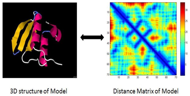
The 3D structure and its corresponding distance matrix of a protein model.

C. Principal component analysis (PCA)

PCA [25] is a widely used statistical method for linear dimensionality reduction using orthogonal transformation. Normally, the input is normalized to zero mean. Then the singular value decomposition is used on input’s covariance matrix to derive eigenvectors and eigenvalues. A subset of eigenvectors can be used to project the input to a lower-dimensional representation. The eigenvalues indicate how much information is retained when reducing the dimensionality of the input.

D. Deep Learning with Sparse Autoencoder

An autoencoder [26–29] is a Feedforward Neural Network (FFNN) that tries to implement an identity function by setting the outputs equal to the inputs in training. Figure 2 shows an example. A compressed representation of the input data, as represented by the hidden nodes, can be learned by placing some restrictions on the network. One way is to force the network to use fewer nodes to represent the input by limiting the number of nodes in the hidden layer. Each hidden node represents a certain feature of the input data. Autoencoders can be viewed as nonlinear low-dimensional representations as compared to linear low-dimensional representations generated by PCA. In autoencoders, the mapping of the input layer to the hidden layer is called encoding and the mapping of the hidden layer to the output layer is called decoding. In general, an autoencoder of a given structure tries to find the weights to minimize the following objective function:

$$\underset{W,b}{\mathit{argmin}}J(W,b)=\Vert h_{W,b}(x)-x\Vert$$ (4)

where x is the input, W the weights, b the biases, and h the function mapping input to output.

Figure 2.

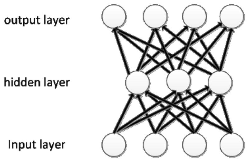
An example of autoencoder

Another technique of forcing an autoencoder to learn compressed representation is sparsity regularization on the hidden nodes, i.e., only a small fraction of hidden nodes are active for an input. With sparsity regularization, the number of hidden nodes can be more than that of the input nodes. Specifically, let

$${\widehat{p}}_j=\frac{1}{m}{\sum }_{i=1}^m[a_j^{(2)}(x^{(i)})]$$ (5)

be the average activation of hidden unit j over a training set of size m. The goal here is to make p̂ approximate a given sparsity parameter p. To measure the difference between p and p̂, an extra penalty term can be added to Eq. (4):

$$R={\sum }_{j=1}^{s_2}\mathit{plog}\frac{p}{{\widehat{p}}_j}+(1-p)\mathit{log}\frac{1-p}{1-{\widehat{p}}_j}$$ (6)

where s₂ is the number of nodes in the hidden layer and j a hidden node. The value reaches minimum of 0 when p̂_j = p and goes to infinity as p̂_j approaches 0 or 1. Now, the overall cost function becomes

$$J_{\mathit{spares}}(W,b)=J(W,b)+\beta R$$ (7)

where parameter β defines the tradeoff between the mapping quality and the sparsity of a network.

Given the objective function in Eq. (7), its derivatives w.r.t. W and b can be derived analytically. Variants of backpropagation algorithms can find optimal W and b values iteratively on training examples.

Stacked autoencoders are deep learning networks constructed using autoencoders layer-by-layer. Another autoencoder can be constructed on top of a trained autoencoder by treating the learned feature detectors in the hidden layer of the trained autoencoder as visible input layer. Autoencoder training is unsupervised learning since only unlabeled data are used. The learned weights and biases will be used as the starting point for the fine-tuning supervised learning stage of deep learning.

The supervised learning stage adds a label layer, such as a softmax classifier, as the highest layer. First, the softmax classifier is trained using labeled data. Then the whole multilayer deep network is treated as a feedforward network and trained using backpropagation, starting with weights and biases learned before.

III. DL-Pro, A Novel Deep Learning Method for Protein Model QA

A. Problem formulation

The QA problem is formulated as a classification problem in this paper: given a set of predicted models of a protein, classify them into two classes, good (or near-native) and bad.

For the experiments, we prepare the dataset that contains good and bad models, but not intermediate models, as follows. Let A be a set of n predicted models for a target protein of length l, A={a_i, 1 ≤ i ≤ n}, and a_i = {U^j, j ∈ [1,l]} where U^j is the 3D coordinates of residue j of model a_i. Let C = {c_i, 1 ≤ i ≤ n, 0 ≤ c_i ≤ 1} be the true-GDT_TS scores, i.e. the true quality, of models in A. Then, the classification label of a model is P (for near native) if its true GDT_TS score c_i ≥ 0.7, and label P̄ (for not near native) if its true GDT_TS score c_i < 0.4. Note that models with true GDT_TS scores between 0.4 and 0.7 are dropped from the dataset. Our focus in the paper is to separate clearly good models from clearly bad models.

In this paper, the performance metric of a classification algorithm is classification accuracy T:

$$T=\frac{v}{n}$$ (8)

where v is the number of correctly classified examples and n is the total number of examples.

B. Classification using energy or scoring functions

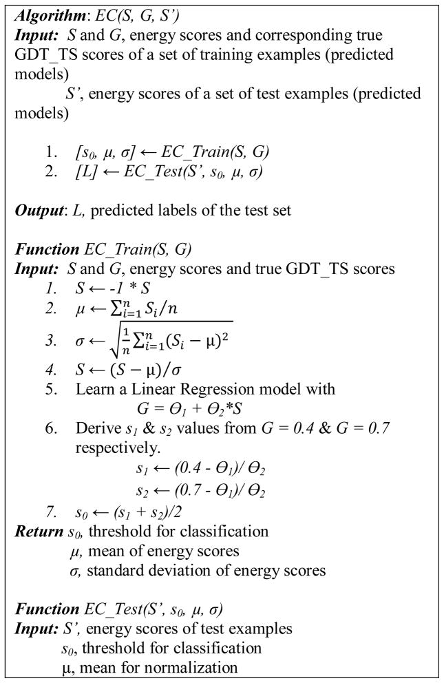
For comparison purpose, we adapt existing energy or scoring functions for the classification problem defined in the previous subsection. The general method, call EC (Energy function based Classification), can be applied to existing energy or scoring functions, including the four used in this paper, OPUS-CA, DOPE, DFIRE, and RW. For these four scoring functions, smaller values represent better models and near-native models have very negative values. Since the true GDT_TS scores of models are in the range [0–1] and larger value means better, a linear mapping from energy scores to the true GDT_TS scores is first learned from a set of training examples and then the thresholds corresponding to good (true GDT_TS score ≥ 0.7) and bad (true GDT_TS score c_i < 0.4) models are determined. Later, the energy scores of test examples are first converted using the linear mapping and then their classes are determined using the learned thresholds.

Figure 3 shows the pseudocode of the EC algorithm. The algorithm consists of a training phase, EC_Train, and a test phase, EC_Test. Based on the energy scores and corresponding true GDT_TS scores of a set of models, which constitute the training examples, EC_Train first computes the mean and standard deviation of the energy scores for normalization, performs linear regression, and then determines a threshold to label the positive (good) and negative (bad) examples.

Figure 3.

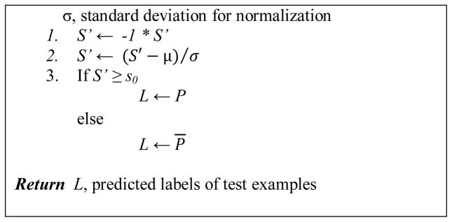
Pseudocode of the EC (Energy function based Classification) algorithm.

Specifically, EC_Train first flips the sign of energy scores from negative to positive so that bigger value means better. Then energy scores are normalized to zero mean and unit variance. Next, a linear function with parameters Θ₁ and Θ₂ is learned to fit the data of normalized energy scores and true-GDTTS scores. Two values, s₁ and s₂, on the normalized energy scores are calculated using the linear function from true GDTTS scores 0.4 and 0.7. Finally, the average of s₁ and s₁, s_0, is the threshold on energy scores for labeling the two classes, good and bad models.

On test examples, EC_Test first normalizes the energy score of a test example using the training example mean and standard deviation. Then, the example gets a positive label if the normalized energy score is larger than the threshold s₀ and gets a negative label otherwise.

C. New QA methods based on C-α atom distance matrix

In this section, a new approach based on C-α atoms distance matrix and machine learning methods is proposed for single-model quality assessment and the identification of native-like models. Different from existing energy/scoring functions and consensus approaches, this new approach is purely geometry based. Various supervised machine learning algorithm can be used in this approach and three algorithms based on deep learning networks, support vector machines (SVM), and feed-forward neural networks (FFNN), respectively, are presented next.

1) DL-Pro, a new deep learning QA algorithm using C-α atom distance matrix

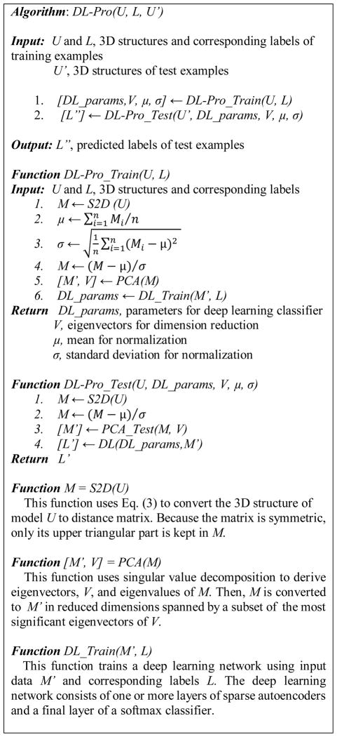
DL-Pro is a novel QA algorithm based on deep learning techniques. For a protein model, DL-Pro uses its distance matrix that contains pairwise distances between two residues’ C-α atoms in the model, which sometimes is also called contact map, as an orientation-independent representation. From training examples of distance matrices corresponding to good and bad models, DL-Pro learns a stacked sparse autoencoder classifier to classify good and bad models.

Figure 4 shows the pseudocode of the DL-Pro algorithm. DL-Pro consists of a training phase, DL-Pro_Train, and a test phase, DL-Pro_Test. Based on the 3D structures and labels of a set of training models, DL-Pro_Train first computes the distance matrix composed of pairwise distances between every pair of residues’ C-α atoms in the model. Then, the distance matrix is normalized to mean 0 and standard deviation 1 based on its mean and standard deviation, which are kept for future use in testing. Next, PCA is applied to reduce the dimension of the distance matrices to generate the inputs of training examples. Significant reduction can be achieved even when 99% of information is kept, i.e., keeping 99% variance of the original data set.

Figure 4.

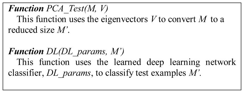
Pseudocode of the DL-Pro algorithm, a novel QA algorithm based on deep learning and model distance matrix of pairwise distances between two residues’ C-α atoms in a model.

The top eigenvectors are kept for future use in testing. Finally, a deep learning network consisting of one or more layers of sparse autoencoders followed by a softmax classifier is trained using the training examples.

On test examples, DL-Pro_Test first pre-processes a test model by calculating its distance matrix, normalizing the matrix using learned mean and standard deviation, and reducing the matrix dimension using PCA with learned eigenvectors. Then, the learned deep learning network classifier is used to classify the data.

2) A new Support Vector Machine (SVM) QA algorithm using C-α atom distance matrix

Instead of stacked autoencoder classifiers, other classifiers such as SVM can also be used in the approach based on C-α atom distance matrix. The algorithm using SVM is very similar to the DL-Pro algorithm in Figure 4, with only two differences: 1) Step 6 of DL-Pro_Train is replaced by training a SVM classifier using the examples to get SVM parameters. 2) Step 4 of DL-Pro_Test is replaced by SVM classification [30].

3) A new Feedforward Neural Network (FFNN) algorithm using C-α atom distance matrix

In this algorithm, FFNNs, instead of deep learning classifiers or SVMs, are used to perform supervised learning and classification. Again, Step 6 of DL-Pro_Train and Step 4 of DL-Pro_Test are replaced by FFNN training and testing.

IV. EXPERIMENTAL RESULTS

1) Data set

CASP dataset: 20 CASP targets with sequence length from 93 to 115 are selected. Each target has approximately 200 predicted models. To reduce redundancy, all models that have the same GDT_TS score are removed. All models shorter than 93 residues are also removed. To make all examples the same input size, all models longer than 93 are truncated at the beginning and end, and the middle segment of 93 residues are kept. In the end, the dataset has good and bad 1,117 models.

Protein native structure dataset: The native structures of a set of protein with sequence length from 93 to 113 are downloaded from Protein Data Bank’s website. These native structures are compared with the native structures of the 20 CASP targets selected. If a native structure is more than 80% similar to a CASP target, it is removed to make sure that the training set and test set used in our experiments do not overlap. Similarly to the CASP set, structures longer than 93 are truncated on both ends to get to 93. In the end, the dataset has 972 structures.

For a model of length 93, the size of the upper triangle portion of the 93 by 93 distance matrix is 4278, a very high dimensional input to a typical classifier. After applying PCA with 99% information retained, the input dimension is reduced to 358, much more manageable.

2) Classification performance of energy functions

In this experiment, the EC (Energy function based Classification) algorithm in Figure 3 is applied to the CASP dataset with different energy scores obtained from OPUS-CA, DOPE, DFIRE, and RW, respectively. The experiment results are from 4-fold cross-validation: the dataset is divided into 4 folds, each containing models of 5 targets. The EC algorithm is run 4 times total, each using 3 folds as training examples and 1 fold as test examples. The final result is the average of the 4 runs.

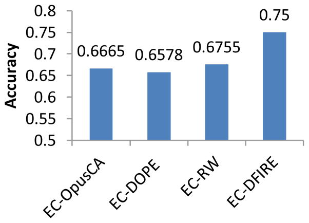
Figure 5 shows classification accuracy of the four energy function based algorithms. EC-DFIRE achieves the best performance, 75% accuracy, while the other three have similar results, around 66%. Table 1 shows the confusion matrix of EC-DFIRE. Positive examples are predicted very accurately, 660 out of 740, 89%, whereas prediction accuracy on negative examples is much lower, 182 out of 375, 49%.

Figure 5.

Classification performance of energy function based classification algorithms. The EC algorithm in Figure 3 is applied to the CASP dataset with different energy scores obtained from OPUS-CA, DOPE, DFIRE, and RW, respectively.

Table 1.

Confusion matrix of EC-DFIRE on the CASP dataset

	Predicted Positive	Predicted Negative
Actual Positive	660	82
Actual Negative	193	182

3) Classification performance of QA algorithms based on C-α atom distance matrix: DL-Pro, SVM, and FFNN

In this experiment, the CASP dataset is again divided into 4 folds, each containing models of 5 targets, and the results of 4-fold cross-validation are reported. The SVM and FFNN algorithms only use the CASP dataset, whereas DL-Pro uses something extra, the protein native structure dataset, in its unsupervised autoencoder learning stage.

For the FFNN algorithm, 1 hidden layer networks with different hidden units (25, 50, 100, 150, 200, and 250) were tried. For the DL-Pro algorithm, 1 and 2 hidden layer networks were tried. For 1-hidden-layer configurations (referred to as DL-Pro1), various numbers of hidden units (50, 100, 150, 200, and 250) were tried. For 2-hidden-layer configurations (referred to as DL-Pro2), the first hidden layer is fixed at 300 hidden units, while the 2^nd hidden layer has various numbers of hidden units (100, 200, 300, 400, and 500). Other parameters are listed in Table 2. For each configuration, DL-Pro and FFNN ran for 10 times from random initial weights and their average results are reported.

Table 2.

Parameters of sparse autoencoder training in the DL-Pro algorithm used in the experiments.

Parameter	Value
Sparsity	0.1
Weight decay λ	3e-3
Weight of sparsity penalty β	3
Maximum number of iterations	500
Optimization method	‘lbfgs’

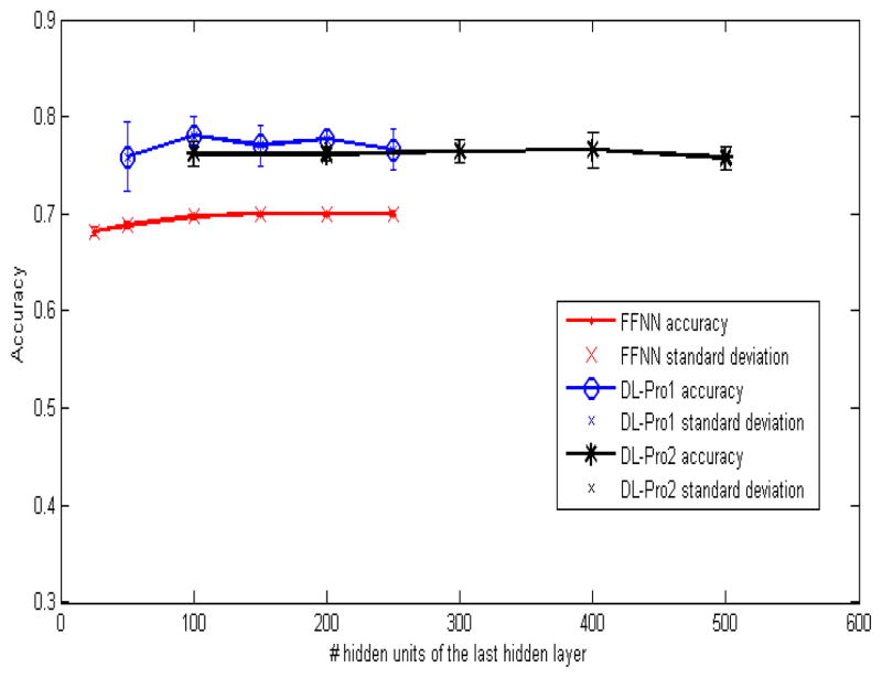
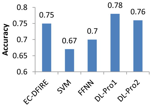
Figure 6 shows classification accuracy of DL-Pro1 (DL-Pro with one-hidden-layer configurations), DL-Pro2 (DL-Pro with two-hidden-layer configurations), and FFNN with various hidden units. Their performance changes slightly as the number of hidden units changes. DL-Pro1 with 100 hidden units yields the best result with accuracy of 0.78. Figure 7 compares classification performance of EC-DFIRE (the best of energy functions), SVM, FFNN, DL-Pro1 and DL-Pro2. SVM is significantly worse than FFNN and DL-Pro algorithms. Both DL-Pro1 and DL-Pro2 are slightly better than EC-DFIRE, with DL-Pro1 achieving 78% accuracy, the best overall. The performance difference between FFNN and DL-Pro shows that deep learning is able to learn better features from both labeled and unlabeled data to achieve improved performance over traditional neural networks.

Figure 6.

Classification performance of DL-Pro1 (DL-Pro with one-hidden-layer configurations), DL-Pro2 (DL-Pro with two-hidden-layer configurations), and FFNN with various hidden units.

Figure 7.

Classification performance of EC-DFIRE (the best of energy functions), SVM, FFNN, DL-Pro1 and DL-Pro2.

Table 3 shows the confusion matrix of SVM, indicating that it classifies all examples as positive. Table 4 shows the confusion matrix of FFNN with 1 hidden layer of 150 hidden units. Its accuracy is 81% on positive examples and 47% on negative examples. Finally, Table 5 shows the confusion matrix of DL-Pro1 with 1 hidden layer of 100 hidden units. Its accuracy on positive examples is excellent, 95%, but not so good on negative examples, only 45%.

Table 3.

Confusion matrix of the SVM QA algorithm based on C-α atom distance matrix

	Predicted Positive	Predicted Negative
Actual Positive	742	0
Actual Negative	375	0

Table 4.

Confusion matrix of FFNN with 1 hidden layer of 150 hidden units.

	Predicted Positive	Predicted Negative
Actual Positive	604	138
Actual Negative	198	177

Table 5.

Confusion matrix of DL-Pro1 with 1 hidden layer of 100 hidden units.

	Predicted Positive	Predicted Negative
Actual Positive	704	38
Actual Negative	207	168

V. Summary

This paper presents a new approach based on C-α atoms distance matrix and machine learning methods for single-model QA. To the best of our knowledge, this is the first attempt to use purely geometry information of a model and deep learning for single-model QA. Three new QA algorithms, DL-Pro, FFNN, and SVM using different learning methods have been proposed within the common framework.

Experiments using selected CASP models and targets show very promising results. Compared to traditional feedforward neural networks, deep learning is significantly better, as demonstrated by the performance difference between DL-Pro and FFNN. Deep learning was able to learn useful features representing good models and DL-Pro achieved the best results, outperforming state-of-the-art energy/scoring functions, including DFIRE, OPUS-CA, DOPE, and RW. Yet, the information used by DL-Pro is far less than other single-model QA methods. With additional model information, DL-Pro is expected to improve further.

References

- 1.Johnson MS, Srinivasan N, Sowdhamini R, Blundell TL. Knowledge-based protein modeling. Crit Rev Biochem Mol Biol. 1994;29:1–68. doi: 10.3109/10409239409086797. [DOI] [PubMed] [Google Scholar]
- 2.Sali A, Blundell TL. Comparative protein modelling by satisfaction of spatial restraints. J Mol Biol. 1993 Dec 5;234(3):779–815. doi: 10.1006/jmbi.1993.1626. [DOI] [PubMed] [Google Scholar]
- 3.Söding J, Biegert A, Lupas AN. The HHpred interactive server for protein homology detection and structure prediction. Nucleic Acids Res. 2005 Jul 1;33(Web Server issue):244–8. doi: 10.1093/nar/gki408. [DOI] [PMC free article] [PubMed] [Google Scholar]
- 4.Zhang Y. I-TASSER server for protein 3D structure prediction. BMC Bioinformatics. 2008 Jan 23;9:40. doi: 10.1186/1471-2105-9-40. [DOI] [PMC free article] [PubMed] [Google Scholar]
- 5.Kim DE, Chivian D, Baker D. Protein structure prediction and analysis using the Robetta server. Nucleic Acids Res. 2004 Jul 1;32(Web Server issue):W526–31. doi: 10.1093/nar/gkh468. [DOI] [PMC free article] [PubMed] [Google Scholar]
- 6.Zhang J, Wang Q, Barz B, He Z, Kosztin I, Shang Y, Xu D. MUFOLD: A new solution for protein 3D structure prediction. Proteins. 2010 Apr;78(5):1137–1152. doi: 10.1002/prot.22634. [DOI] [PMC free article] [PubMed] [Google Scholar]
- 7.Wang Q, Vantasin K, Xu D, Shang Y. MUFOLD-WQA: A New Selective Consensus Method for Quality Assessment in Protein Structure Prediction. Proteins. 2011;79(Suppl 10):185–195. doi: 10.1002/prot.23185. [DOI] [PMC free article] [PubMed] [Google Scholar]
- 8.Benkert P, Tosatto SC, Schwede T. Global and local model quality estimation at CASP8 using the scoring functions QMEAN and QMEANclust. Proteins. 2009;77(Suppl 9):173–80. doi: 10.1002/prot.22532. [DOI] [PubMed] [Google Scholar]
- 9.Cheng J, Wang Z, Tegge AN, Eickholt J. Prediction of global and local quality of CASP8 models by MULTICOM series. Proteins. 2009;77(Suppl 9):181–4. doi: 10.1002/prot.22487. [DOI] [PubMed] [Google Scholar]
- 10.Wu Y, Lu M, Chen M, Li J, Ma J. OPUS-Ca: A knowledge-based potential function requiring only Ca positions. Protein Science. 2007;16(7):1449–1463. doi: 10.1110/ps.072796107. [DOI] [PMC free article] [PubMed] [Google Scholar]
- 11.Zhang J, Zhang Y. A Novel Side-Chain Orientation Dependent Potential Derived from Random-Walk Reference State for Protein Fold Selection and Structure Prediction. PLoS ONE. 2010;5(10):1–13. doi: 10.1371/journal.pone.0015386. [DOI] [PMC free article] [PubMed] [Google Scholar]
- 12.Zhou H, Zhou Y. Distance-scaled, finite ideal-gas reference state improves structure-derived potentials of mean force for structure selection and stability prediction. Protein Sci. 2002 Nov;11(11):2714–26. doi: 10.1110/ps.0217002. [DOI] [PMC free article] [PubMed] [Google Scholar]
- 13.Shen MY, Sali A. Statistical potential for assessment and prediction of protein structures. Protein Sci. 2006 Nov;15(11):2507–24. doi: 10.1110/ps.062416606. [DOI] [PMC free article] [PubMed] [Google Scholar]
- 14.Kryshtafovych A, Fidelis K, Tramontano A. Evaluation of model quality predictions in CASP9. Proteins. 2011;79(Suppl 10):91–106. doi: 10.1002/prot.23180. [DOI] [PMC free article] [PubMed] [Google Scholar]
- 15.Kryshtafovych A, 1, Barbato A, Fidelis K, 1, Monastyrskyy B, Schwede T, Tramontano A. Assessment of the assessment: Evaluation of the model quality estimates in CASP10. Proteins: Structure, Function, and Bioinformatics. 2013 Aug; doi: 10.1002/prot.24347. [DOI] [PMC free article] [PubMed] [Google Scholar]
- 16.Skolnick J. In quest of an empirical potential for protein structure. Curr Opin Struct Biol. 2006;16:166–171. doi: 10.1016/j.sbi.2006.02.004. [DOI] [PubMed] [Google Scholar]
- 17.Brooks BR, Bruccoleri RE, Olafson BD, States DJ, Swaminathann S, Karplus M. Charmm a program for macromolecular energy, minimization, and dynamics calculations. Journal of Computational Chemistry. 1982;4:187–217. [Google Scholar]
- 18.Duan Y, Wu C, Chowdhury S, Lee MC, Xiong G, Zhang W, Yang R, Cieplak P, Luo R, Lee T, Caldwell J, Wang J, Kollman P. A point-charge force field for molecular mechanics simulations of proteins based on condensed-phase quantum mechanical calculations. Journal of Computational Chemistry. 2003;24(16):1999–2012. doi: 10.1002/jcc.10349. [DOI] [PubMed] [Google Scholar]
- 19.Lu H, Skolnick J. A distance-dependent atomic knowledge-based potential for improved protein structure selection. Proteins. 2001 Aug 15;44(3):223–32. doi: 10.1002/prot.1087. [DOI] [PubMed] [Google Scholar]
- 20.Gohlke H, Hendlich M, Klebe G. Knowledge-based scoring function to predict protein-ligand interactions. J Mol Biol. 2000 Jan 14;295(2):337–56. doi: 10.1006/jmbi.1999.3371. [DOI] [PubMed] [Google Scholar]
- 21.Qiu J, Sheffler W, Baker D, Noble WS. Ranking predicted protein structures with support vector regression. Proteins. 2008 May 15;71(3):1175–82. doi: 10.1002/prot.21809. [DOI] [PubMed] [Google Scholar]
- 22.Anjum C. Protein Tertiary Model Assessment Using Granular. 2012 [Google Scholar]
- 23.Wang Q, Shang Y, Xu D. Improving a Consensus Approach for Protein Structure Selection by Removing Redundancy. IEEE/ACM transactions on computational biology and bioinformatics. 2011;8(6):1708–1715. doi: 10.1109/TCBB.2011.75. [DOI] [PubMed] [Google Scholar]
- 24.Zemla A. LGA: a method for finding 3D similarities in protein structures. Nucleic acids research. 2003;31:3370–3374. doi: 10.1093/nar/gkg571. [DOI] [PMC free article] [PubMed] [Google Scholar]
- 25.Hotelling H. Analysis of a complex of statistical variables into principal components. J Educ Psych. 1933;24:417–441. 498–520. [Google Scholar]
- 26.Le Cun Y. PhD Dissertation. PARIS: 1987. Modeles Connexionnistes de L’Apprentissage; p. 6. [Google Scholar]
- 27.Bourlard H, Kamp Y. Auto-Association by multilayer perceptrons and singular value decomposition. Biological cybernetics. 1988;59:291–294. doi: 10.1007/BF00332918. [DOI] [PubMed] [Google Scholar]
- 28.Hinton GE, Zemel RS. Autoencoders, minimum description length, and helmholtz free energy. Advances in Neural Information Processing. 1994:3–10. [Google Scholar]
- 29.Ng A. Sparse autoencoder. Lecture note. Available online at: http://www.stanford.edu/class/cs294a/sparseAutoencoder.pdf.
- 30.Ng A. Support Vector Machine. Lecture note. Available online at: http://cs229.stanford.edu/notes/cs229-notes3.pdf.