Measuring the Displacement and Replacement of Government Health Expenditure

Abstract

Research assessing the relationship between government health expenditure and development assistance for health channeled to governments (DAHG) has not considered that this relationship may depend on whether DAHG is increasing or decreasing. We explore this issue using general method of moments estimation and a panel of financial flows data spanning 119 countries and 16 years. Our primary concern is how DAHG affects government health expenditure as source (GHES). We disaggregate the average effect of DAHG and separately identify the effects of increases versus decreases in DAHG. We find that a $1 year-over-year increase in DAHG leads to a $0.62 (90% confidence interval (CI): 0.15, 1.09) decrease in GHES, whereas a $1 year-over-year decrease in DAHG does not have an effect on GHES that is statistically different from zero (CI: −0.67, 1.17). Simulation shows that the displacement of GHES between 1995 and 2010 reduced total government health expenditure by $152.8 billion (CI: 46.9, 277.6). Moreover, the irregular disbursement of DAHG reduced total government expenditure by $96.9 billion (CI: 0.5, 212.4). Thus, this research shows that health aid is fungible and highlights the cost of displacement and erratic aid disbursement.

1. Introduction

Governments finance a sizable portion of population health initiatives throughout the world. Government resources fund public health systems, health services, and public insurance schemes. In 2010, governments spent roughly $4.05 trillion on health, although these resources are not distributed uniformly across the globe (World Health Organization, 2012; Institute for Health Metrics and Evaluation, 2013).¹ Eighty-five percent of this total is spent in high-income countries, where approximately 15% of the world’s population lives (United Nations Population Division, 2011). To address health financing gaps in many low-income and middle-income countries, domestically generated government health expenditure is complemented by development assistance for health (DAH). In 2010, DAH totaled $28.2 billion, with 47% of the DAH that can be tracked to specific countries channeled to governments (denoted as DAHG) (Institute for Health Metrics and Evaluation, 2013).

For most donors, the implicit (and sometimes explicit) intention of DAHG is to increase the total amount of governmental spending on health. In other words, donors intend for governments to maintain their own health spending while they receive DAHG. However, governments have competing priorities, and DAHG may crowd out domestic health spending. When a government receives DAHG, it might redirect government health expenditure as source (GHES, or the domestically generated portion of total government health expenditure). In these cases, DAHG is fungible and not fully additional, meaning $1 of DAHG does not lead to an increase of $1 in total health expenditure. Some empirical research shows this to be the case (Farag et al., 2009; Lu et al., 2010; Fernandes Antunes et al., 2012; Dieleman et al., 2013). Although these findings coincide with some economic theory and empirical studies that assess other government sectors (Pack and Pack, 1993, 1990; Feyzioglu et al., 1998; Oates, 1999; Swaroop et al., 1999, 2000; McGillivray and Morrissey, 2001; Dodd et al., 2007; Wagstaff, 2011), other research questions these conclusions (Roodman, 2012; Van de Sijpe, 2013). In order to assess and predict resources for health and any potential health gains, knowing how financial flows interact is of the utmost importance.

Furthermore, an assessment of the relationship between DAHG and GHES should provide more than just a single aggregated estimate of the effect. The rate at which governments displace GHES with DAHG might differ across many dimensions, including the type of DAHG or the organization of the country’s health system. Yet, another dimension that might dictate a government’s rate of displacement is how the present amount of DAHG relates to previous amounts disbursed. It is plausible that aid recipients might respond asymmetrically to increases and decreases in resources, especially if reallocating funds across sectors is costly. The prevailing assumption is that if DAHG is fungible, then governments replace GHES upon decreases in DAHG at the exact same rate that they displace GHES upon increases in DAHG. If displacement does not equal replacement, then the effects of a short-run DAHG shock could persist beyond the length of the shock itself.

To assess these issues, we construct a panel of cross-country GHES and DAHG data similar to what is constructed by Dieleman et al. (2013). Dieleman et al. 2013 provides evidence that DAHG crowds out GHES and that this effect is dynamic. This means that short-run shocks have persistent effects on GHES. To explore why, we disaggregate the average effect of DAHG by separately identifying the effects of increases versus decreases in DAHG. We use general method of moments (GMM) estimation and a specification that is flexible enough to measure the effect of increases and decreases in DAHG separately. Section 2 outlines this estimation and the data we employ. Section 3 reports our results and uses simulation to quantify the estimates’ magnitudes. Section 4 concludes by exploring the policy implications for these findings. A substantive series of robustness checks is available in the online appendix.

2. Methods

2.1. Data and model

The data used in this study span 16 years (1995 through 2010) and 119 countries. DAHG is reported by the Institute for Health Metrics and Evaluation in Financing Global Health 2012: End of the Golden Age? (Institute for Health Metrics and Evaluation, 2013). The World Health Organization reports total government health expenditure data, also known as government health expenditure as agent (GHE) (World Health Organization, 2012). By definition, GHE ≡ GHES + DAHG (World Health Organization, 2003; Lu et al., 2010). Thus, GHES is obtained by subtracting DAHG from GHE. Tables S1 through S4 in the online appendix include a list of countries included in the study, a list of data sources, and summary statistics (James et al., 2012; World Health Organization, 2012; Institute for Health Metrics and Evaluation, 2013).

Model (1) reflects the literature’s current approach to measuring the determinants of GHES (Lu et al., 2010; Dieleman et al., 2013; Van de Sijpe). Table 1 describes the variables included as covariates. All financial variables except gross domestic product (GDP) are measured as a share of the country’s 16-year average GDP. This strategy enables us to correctly identify periods when GHES is increasing or decreasing in absolute terms. (If the variables were measured as a share of contemporaneous GDP, then periods when DAHG increased at a slower rate than GDP would incorrectly appear to have declining levels of DAHG.) DAHNG is DAH that is not determined to be channeled to the recipient country’s government, whereas GROWTH is the GDP growth rate. GDP and population (POP) are natural log transformed. Unobserved country-level heterogeneity exists in our panel and is controlled for by the inclusion of country-level fixed effects (α_i). Time indicators control for the trend of increasing government expenditure on health and idiosyncratic shocks across our panel (τ_t). Subscripts i and t indicate country and year of each observation.

(1)

Whereas model (1) represents a common approach used to measure health aid fungibility, we estimate model (2). Only one feature distinguishes model (2) from model (1). DAHG is parsed into two distinct variables: DAHG and DAHG⁻. DAHG⁻ is the interaction between DAHG and a binary indicator marking a year-over-year decrease in DAHG. (DAHG^- is thus zero for all country-years where DAHG is the same as or larger than the previous year.) By modeling increases and decreases in DAHG separately, model (2) measures the displacement and replacement of GHES without assuming these two rates are equal. is the estimated displacement rate (which follows an increase in DAHG), whereas is the estimated replacement rate (which follows a decrease in DAHG). A Wald test is used to assess the hypothesis that the coefficient is statistically different from zero. Rejecting this hypothesis is the same as rejecting and confirms governments displace and replace GHES at statistically different rates.

(2)

Table 1.

Definitions of variables

Abbreviation	Variable
GHESit	Government health expenditure as source; measured as a percentage of the country’s mean GDP for country i in year t
DAHGit	Development assistance for health channeled to a government; measured as a percentage of the country’s mean GDP for country i in year t
DAHNGit	Development assistance for health not channeled to a government; measured as a percentage of the country’s mean GDP for country i in year t
GGEit	General government expenditure, net of government health expenditure as source; measured as a percentage of the country’s mean GDP for country i in year t
GDPit	Gross domestic product; measured per capita and log transformed for country i in year t
POPit	Population for country i in year t; log transformed
GROWTHit	Annual percentage change in GDP for country i in year t
αi	Unobserved time-invariant country-specific characteristics (fixed effects)
τt	Unobserved idiosyncratic time shock (fixed effects)
εit, νit	Error term for country i in year t

2.2. Estimation

The Wooldridge test is used to identify autocorrelation in GHES. The null hypothesis is that no autocorrelation exists (Wooldridge, 2001; Drukker, 2003). We find that hypothesis is soundly rejected (p < 0.001). To deal with autocorrelation, we include a 1-year lag of the dependent variable (LDV). To avoid introducing the bias common in short panels that include fixed effects and an LDV, we use two-step system GMM estimation (Nickell, 1981; Arellano and Bond, 1991; Arellano and Bover, 1995; Blundell and Bond, 1998). System GMM uses internally derived instruments to control for endogenous variables. This estimator is ideal for repeated panels with few time periods where autocorrelation within countries, unobserved fixed effects across countries, and endogenous independent variables could otherwise bias the results (Roodman, 2009). We treat DAHG, DAHNG, and the LDV as endogenous because of the statistical relationship binding these variables to GHES. (See Dieleman et al. 2013 for more detail.)

A common problem with system GMM is the proliferation of instruments. Over-instrumenting can simultaneously over-fit endogenous variables and weaken the test used to assess the exogeneity of the instrument set (Roodman, 2007). We simultaneously employ two methods to address this problem. We ‘collapse’ the instrument set (Roodman, 2007, 2009) and use principal components analysis to factor the instrument set (Roodman, 2009; Bai and Ng, 2010). Simulation shows that when combined, these techniques minimize bias (Mehrhoff, 2009).

Two tests support the validity of the internal instruments used in system GMM. First, we use the Arellano–Bond test to identify the degree to which autocorrelation exists after country-level fixed effects are parsed out (Arellano and Bond, 1991; Roodman, 2009). If autocorrelation is present, then part of the instrument set is not valid. The null hypothesis is that no autocorrelation exists. Second, we use the Hansen J test to test the exogeneity of the instrument set. The null hypothesis is that the full instrument set is exogenous. As the p-value for this test moves toward zero, causal claims become tenuous.

2.3. Robustness

We assess the sensitivity of the results across a wide set of alternative datasets, estimation specifications, variable specifications, and estimation methods. We complete more than 200 additional regressions. Each additional regression varies a single component of the estimation. These results provide evidence that the baseline results are robust. For further description of these methods, primary results, and sensitivity analyses, see Tables S5 through S20 and Figures S1 and S2 in the online appendix.

3. Results

Table 2 reports our primary results. These estimates show that health aid channeled to the government is a significant determinant of government health expenditure. We also find that governments respond to changes in the amount of DAHG disbursed in an asymmetric manner. Increases in DAHG lead to the displacement of GHES, whereas decreases in GHES do not on average lead to replacement. For every $1 increase in DAH, GHES decreases by $0.62 (90% confidence interval (CI): 0.15, 1.09). This is statistically different from zero, with p-value = 0.031. Decreases in DAHG, on the other hand, have a relatively small effect on GHES. For every $1 decrease in DAHG, GHES decreases by $0.25 (CI: −0.67, 1.17). This estimate has the opposite sign we expect and is not statistically different from zero at any conventional level (p = 0.663). With some confidence, we can reject that the displacement rate and the replacement rate are statistically equivalent (p = 0.082). This assessment confirms that it is highly likely that DAHG is being displaced at a larger rate than it is being replaced.

Table 2.

Regression results

Variables	GHES/GDP
Lag GHES/GDP	0.924*** (0.062)
DAHG/GDP	−0.620** (0.287)
DAHG-/GDP	0.865* (0.497)
DAHNG/GDP	0.442* (0.245)
GGE/GDP	0.008* (0.004)
Ln GDP per cap	0.001 (0.001)
GDP growth rate	0.017*** (0.004)
Ln population	0.000 (0.000)
Constant	−0.001 (0.007)
Observations	1762
Number of countries	119
Effect of decrease in DAHG (beta estimate)	0.245
Effect of decrease in DAHG (standard error)	(0.562)
Test up = down p-value	0.082
Hansen p-value	0.272
AR(2) p-value	0.345
Instrument count	37

Two-step system GMM estimation of model (2). Coefficient estimates for time indicators suppressed. DAHG, DAHNG, and LDV treated as endogenous. Instrument matrix is ‘collapsed’ and factored using principal components analysis. Components with eigenvalue greater than one retained. Windmeijer standard errors reported. Forward orthogonal deviation used for the transformed equation, rather than first-differencing. Backward orthogonal deviation used for the instruments of the level equation, rather than first-differencing.

Windmeijer adjusted standard errors in parentheses.

 ***p < 0.01,

 **p < 0.05,

 *p < 0.1.

Table 2 also shows that GHES is dynamic, as the LDV is significantly different from zero (p < 0.001). This means that on average, this year’s level of government spending is a function of last year’s level of spending, and the consequences of changes in GHES determinants persist over time. The long-run effect (total loss of GHES over time) for every $1 increase in DAHG is estimated to be $8.15 (CI: −2.27, 18.57). On the other hand, long-run effect of a decrease in DAHG on GHES is essentially zero, with a long-run effect estimate of $3.22 (CI: −11.11, 17.56).

In addition to reporting the displacement and replacement rates, Table 2 also shows how other determinants affect GHES. GGE, GDP, DAHNG, and GDP growth are all positively associated with GHES. A $1 increase in non-health general government expenditure predicts a $0.01 (CI: $0.00, $0.01) increase in GHES. Whereas the coefficient estimate for GDP is not statistically different from zero (p-value = 0.167), the coefficient estimate for GDP growth is (p < 0.001). An expanding economy predicts a larger government health sector. We also see that increases in DAHNG might drive up health costs. These estimates reflect relationships described previously in this literature and add to the confidence we place in our specification and estimation (Farag et al., 2009; Lu et al., 2010; Xu et al., 2011; Van de Sijpe, 2013). Additionally, the instrument exogeneity tests suggest that our estimation is credible. Neither the Arellano–Bond test nor the Hansen J test provides evidence that our factored instruments are not exogenous (p-values = 0.272 and 0.345, respectively).

To clarify the consequences of this behavior and the uncertainty associated with our estimates, we compare the baseline GHE estimates to three simulated counterfactuals. Each counterfactual uses the baseline model but alters a single input. Table 3 summarizes these counterfactual scenarios. The results are illustrated in Figures 1 through 3.

Table 3.

Three counterfactuals exploring the cost of displacement

Counterfactual	Displacement rate	Replacement rate	Disbursement of DAHG	Cost in billions (90% confidence interval)
1	0	0	As observed	$152.8 billion (CI: 46.9, 277.6)
2	As estimated	Irrelevant	Monotonically increasing	$96.9 billion (CI: 0.5, 212.4)
3			As observed	$78.6 billion (CI: −23.7, 192.1)

Three counterfactuals are considered and compared with the baseline. In the baseline, displacement and replacement rates are those found via estimation, and the disbursement of DAH is as observed. Cost is the difference between baseline GHE and the counterfactuals’ GHE. GHE estimates are aggregated across all 119 countries and years of data. Ninety percent confidence intervals are calculated using 1000 draws from the variance–covariance matrix generated using the baseline estimation.

Figure 1.

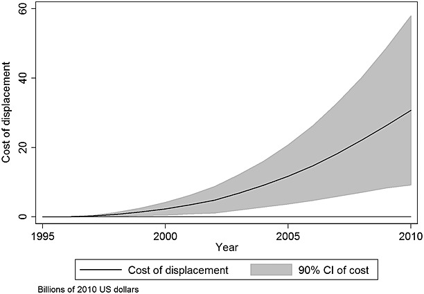
The cost of displacement and replacement between 1995 and 2010. This figure compares the effect of the actual scale-up of DAHG between 1995 and 2010 and a counterfactual. In the counterfactual scenario, recipient countries do not displace (or replace) any resources upon the receipt of DAHG. Cost is defined as the difference between GHE^{NoDisplacement} (modeled assuming displacement = replacement = 0) and GHE^Actual (modeled assuming displacement and replacement rates estimated in model (2)). The cost is positive and significant, showing that had recipient countries not displaced resources, more total government health resources would have been available. The 90% CI is generated taking the 1,000 random draws from the estimated variance–covariance matrix

Figure 3.

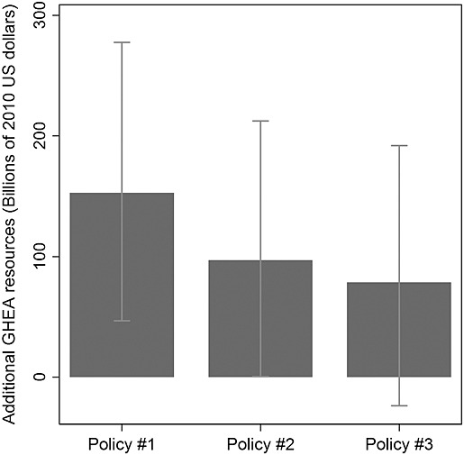
Policy options to limit effects of displacement. Between 1995 and 2010, $43.8 billion of DAHG was disbursed. This figure compares three possible policies that could have been used to insert more resources into the government health sector. Policy #1 is based on methods used to generate Figure 1 and assumes that recipient countries do not displace any DAHG. If policy #1 had been adopted between 1995 and 2010, $152.8 billion (CI: 46.9, 277.6) of GHEA would have been preserved. Policy #2 is based on methods used to generate Figure 2 and assumes that donor countries disburse DAHG at a non-decreasing rate. If policy #2 had been adopted between 1995 and 2010, $96.9 billion (CI: 0.5, 212.4) of GHEA would have been preserved. Policy #3 assumes that recipients displaced and replaced increases and decreases in DAHG at the same expected rate of displacement, where the expected rate of displacement is 1 − (GHE / GGE). If policy #3 had been adopted between 1995 and 2010, $78.6 billion (CI: −23.7, 192.1) of GHEA would have been preserved. Thin gray lines reflect the 90% CI.

Figure 1 illustrates the cost of displacement. This figure, based on the estimates presented in Table 2, compares two different scenarios: GHE^Actual and GHE^{NoDisplacement}. GHE^Actual is total (modeled) government health expenditure, including both domestic and foreign components, and is based on actual aid disbursements. GHE^{NoDisplacement} is a counterfactual that assumes a policy where recipient governments did not displace any DAHG between 1995 and 2010. We calculate the cost of displacement by subtracting GHE^Actual from GHE^{NoDisplacement}. Over time, displacement has an increasing cumulative effect on GHE because of disproportionally low replacement rates and the dynamic nature of GHES. The 1-year cost of displacement grows to $30.7 billion (CI: 9.2, 58.0) in 2010, and we estimate that the total cost of displacement (the integral below the curve illustrated in Figure 1) for the 119 countries and 16 years is $152.8 billion (CI: 46.9, 277.6).

Figure 2 illustrates an alternative comparison, the cost of sporadic DAHG disbursements. As in Figure 1, GHE^Actual is the modeled value of GHE. Unlike Figure 1, GHE^Actual is compared with GHE^Smooth in Figure 2. GHE^Smooth envisions a second counterfactual. Rather than assuming recipients do not displace, GHE^Smooth assumes that donors disbursed DAHG at a monotonically increasing amount. Thus, GHE^Smooth does not incur the loss associated with incomplete replacement, because replacement never occurs when DAHG is only increasing. In this scenario, each country receives its own country-specific 16-year aggregate level of DAHG so that the two scenarios differ only in the timing over which the DAHG was disbursed. For Figure 2, the cost of sporadic DAHG is calculated by subtracting GHE^Actual from GHE^Smooth. Figure 2 shows the cost of displacement accrues over time with an increasing gap between GHE^Actual and GHE^Smooth. In 2010, the cost of 16 years of sporadic disbursement leads to a 1-year cost of $21.3 billion (CI: 1.5, 45.1), and we estimate that the total cost of sporadic disbursement (the integral below the curve illustrated in Figure 2) for the 119 countries and 16 years is $96.9 billion (CI: 0.5, 212.4).

Figure 2.

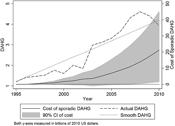
The cost of sporadic disbursement of DAHG between 1995 and 2010. This figure compares the effect of the actual scale-up of DAHG between 1995 and 2010 and a counterfactual. In the counterfactual scenario, the total amount of DAHG disbursed per country is set to be the total amount actually received, but disbursement is set to only increase over time (there are no DAHG reductions). The black solid line shows the cost of sporadically disbursed DAHG. Cost is defined as the difference between GHE^Smooth (caused by smooth DAHG disbursement) and GHE^Actual (caused by actual DAHG disbursement). The cost is positive and significant, showing that a smooth DAHG scale would have led to more total government health resources. The 90% CI is generated taking the 1,000 random draws from the estimated variance–covariance matrix

While not displacing DAHG (Figure 1) and disbursing DAHG at a stable rate (Figure 2) are two policy options that mitigate the adverse effects of displacement, a third policy option is that recipient governments could displace and replace DAHG at an equal rate. Here, we hypothesize that government displacement and replacement could be based on the share of total government expenditure devoted to health (displacement rate = replacement rate = ). This behavior assumes that allocations and reallocations across sectors are costless. While potentially more politically tractable, we calculate that this policy would mitigate less cost. We estimate that the total cost of asymmetric recipient behavior for the 119 countries and 16 years is $78.6 billion (CI: −23.7, 192.1), but this estimate is not statistically significant at any conventional level. Figure 3 compares the accumulated benefit of all three policy alternatives.

The supplementary appendix reports a series of over 200 robustness checks. The vast majority of these estimates support the results presented here. In this paper, we report only one check for robustness—Table 4. This is of special interest because it shows that our results are not a function of our instruments. This table compares our baseline results to the results from two alternative specifications. Because system GMM instruments are a function of the specification, each specification employs different instruments. In our baseline model (model (2)), we regress GHES on DAHG and DAHG⁻, is our estimate of the displacement rate, and is our estimate of the replacement rate. We now regress GHES on DAHG and DAHG⁺ (alternative #1) and also regress GHES on DAHG⁺ and DAHG⁻ (alternative #2). Each specification follows system GMM convention, using transformed time lags to instrument the non-transformed equation, and uses non-transformed time lags to instrument the transformed equation. If our results were a function of relatively weak instruments, then we would expect the results to vary dramatically across these alternative specifications. The stability of our results across the three columns of Table 3 shows that our findings are not a function of our instruments. All three specifications show statistically significant displacement (all three p < 0.05), statistically insignificant replacement (all three p > 0.5), and statistically different displacement and replacement rates (all three p < 0.1).

Table 4.

Displacement and replacement rates across alternative specifications

	Baseline	Alternative #1	Alternative #2
Displacement rate	−0.620** (0.287)	−0.521*** (0.199)	−0.435*** (0.117)
Replacement rate	0.245 (0.562)	0.332 (0.418)	0.257 (0.432)
Displacement = replacement: p-value	0.082	0.040	0.059
Hansen J: p-value	0.272	0.597	0.595
AR(2): p-value	0.345	0.285	0.398

Comparing two alternative specifications to the baseline specification. The baseline specification regresses GHES on DAHG and DAHG⁻. Alternative #1 regresses GHES on DAHG and DAHG⁺. Alternative #2 regresses GHES on DAHG⁺ and DAHG⁻. Displacement rate is consistently statistically significant, whereas the replacement rate is consistently not statistically significant. The displacement and replacement rates are always statistically different (all three p < 0.1). All three specifications use the baseline estimation method: two-step system GMM, treating all DAHG variables, DAHNG, and the LDV as endogenous, ‘collapsing’ and factoring the instruments. All reported standard errors (in parentheses) are Windmeijer adjusted. Each regression includes time indicators, DAHNG, GGE, GDP, GDP growth, and population as covariates.

 ***p < 0.01,

 **p < 0.05.

4. Discussion

When development assistance displaces government expenditure, the sector-specific net gain is not what it could have been sans displacement. In the short run, only $0.38 (CI: −0.09, 0.85) of every $1 of DAHG is additional, whereas $0.62 (CI: 0.15, 1.09) worth of GHES is displaced. Furthermore, reductions in GHES persist over time, even beyond the period in which DAHG is being disbursed. This research examines why this might be, hypothesizing that displacement of GHES might not be asymmetric. We find some evidence of this asymmetry, as the replacement rate (associated with decreasing DAHG) is less than the original displacement (associated with increasing DAHG). This suggests that a 1-year shock of $1 leaves a government health system with a financing gap much larger than it first appears, as it takes time for government to reallocate resources back to the health system. These results imply that fluctuations and unanticipated reductions in DAHG have serious ramifications for total health sector expenditure in the long run. At a time when the supply of DAH has stagnated, the possibility that displacement imposes financing constraints on the health sector has important and timely ramifications (Institute for Health Metrics and Evaluation, 2011; Leach-Kemon et al., 2011; Glassman, 2012).

These conclusions lead to two clear questions about government behavior. First, why does displacement occur? Economic theory suggests that welfare-maximizing governments allocate resources according to the marginal gains associated with achieving their priorities. If the government receives large amounts of DAH relative to development assistance for non-health sectors, then a rational government might displace GHES (Pack and Pack, 1990, 1993; Feyzioglu et al., 1998; Oates, 1999; McGillivray and Morrissey, 2001; van de Walle and Mu, 2007; Ooms et al.). This outcome assumes that resources are fungible and that moving resources across sectors is not cost-prohibitive. As a consequence, health aid crowds out governments’ own resources for health. In the global scale-up of development assistance, assistance for health grew at a faster rate than assistance to other sectors (Institute for Health Metrics and Evaluation, 2009, 2011). This suggests the relatively dramatic scale-up in health aid could be one explanation for displacement. Still, confirmation of this theory requires detailed financial data that are not currently available. To evaluate relative flows, researchers would need data tracking government expenditure and development assistance channeled to governments disaggregated across all sectors. Without these data, our ability to fully understand this phenomenon is limited.

The second question related to government behavior is why the GHES displacement rate does not equal the replacement rate. One intuitive answer is that it is easier to share a windfall than reallocate funds across sectors during a time of austerity. In general, governments are constrained by finite budgets that must be allocated across many competing priorities. Ceteris paribus, an increase in DAHG leads to a net gain in government resources. This research shows that these gains are not restricted to the health sectors, and the cost of sharing resources across sectors when net gains are positive is relatively small. Indeed, when DAHG increases, 62% (CI: 15%, 109%) of it is effectively shared with non-health sectors. On the other hand, decreases in DAHG cause the government’s budget to contract. Returning displaced funds back to the health sector would necessitate cutting funds from other sectors. This research suggests that is relatively difficult, and thus, policymakers are less successful at achieving it.

Naturally, this research has limitations. First, the estimated effects reflect a global average for 119 countries across 16 years. It would be inappropriate to apply results from this study to any one country in any single year. In an attempt to identify heterogeneous effects across regions, we conducted subset analyses focusing separately on sub-Saharan Africa and South and Eastern Asia (see the online appendix). Small samples prevent precise estimates, but these analyses generally confirm displacement occurs. Second, this study makes no claims about population health or welfare. This study confirms that DAHG displaces GHES with longstanding effects, but it would be incorrect to assume that substitution has a specific effect on population health or welfare. Although it is often assumed that fewer resources in a government’s health sector translate to worse health, it remains possible that displacement has a positive effect on population health or welfare via alternative government sectors (McGillivray and Morrissey, 2001; Wagstaff, 2011). If displaced GHES is substituted into other pro-health sectors such as education, positive health gains might still be achieved (Gakidou et al., 2010; Lu et al., 2010; Sridhar and Woods, 2010). Without project-level data about where displaced funds are being channeled, the welfare and health effects related to subadditionality are ambiguous. A final limitation is in our ability to confidently detect a causal effect. Because we measure GHES by netting DAHG from GHE, identifying the direction of the causal connection is difficult. We believe our estimates and instrumentation provide credible evidence of a causal path connecting DAH to government health expenditure. Furthermore, the extensive set of robustness checks and the simplest economic theories on this topic inform our position that increases in DAHG lead to decreases in GHES. Still, this evidence is not equivalent to the definitive proof that would be provided by a randomized, controlled trial or natural experiment. This research uses the best available statistical methods, expenditure data, and health aid data. However, system GMM is a fragile and complicated estimation method, and future work should continue to critically assess its applicability to this issue.

This research leads to five policy recommendations. First, donors and recipients should work together to maintain stable flows of development assistance. Stable financing has positive implications for projects and allows for more effective long-term planning (Woods, 2005; Cavagnero et al., 2008). Moreover, stable disbursement of DAHG is integral to maintaining consistent levels of health financing and preventing financial gaps caused by displacement of GHES without subsequent replacement. Figures 2 and 3 show that there are significant costs associated with sporadic DAHG disbursement and there would most likely be significant gains if DAHG were disbursed smoothly.

The second recommendation is that recipient governments equate the displacement and replacement rates of GHES. Although competing demands for new resources will always exist, incomplete replacement only punishes the sector for which aid was intended. Fluctuating aid disbursements do not need to lead to such distortion. The asymmetry between displacement and replacement is, presumably, a function of internal politicking rather than a means of increasing population welfare.

The third recommendation is that policymakers, donors, and researchers place more emphasis on tracking domestic and international financial flows. Data limitations force researchers to rely on complicated estimation methods. State-of-the-art estimation methods, specification tests, and sensitivity analyses are poor substitutes for better data. More granular measurements of development assistance and more comparable and transparent measurements of government expenditure could lead to more exact measurement of displacement and replacement. Moreover, improved data would permit analysts to address a number of new questions, including identifying heterogeneous effects of DAHG and the welfare implications of displacement. By improving the tracking of financial flows, researchers, donors, and policymakers could become more aware of which countries are substituting their own resources and where displaced funds are going. A comprehensive database on financial flows related to health would empower researchers to more thoroughly assess which types of flows lead to the greatest health gains and measure the health losses (or gains) associated with displacement and replacement.

The fourth recommendation is that cost-effectiveness analyses of health projects incorporate the long-term costs related to financial flows. Evidence from this study indicates that short-term financing may create long-term financing gaps. Even if future flows are heavily discounted, short-term projects with external, unsustainable funding may have consequential long-term financial consequences. The effectiveness analyses of these projects should assess whether the long-term gains associated with the project offset long-term financial costs imposed on the broader public health system.

Finally, the fifth recommendation is that donors might consider how the health projects they finance align with the country’s priorities. If displacement is a foregone conclusion, then it would be advantageous for donors to align their projects with the recipient’s priorities. This conforms to the Paris Declaration, which encourages ‘increasing alignment of aid with partner countries’ priorities, systems, and procedures and helping the strengthening of their capacities’ (Paris Declaration, 2005). Without such alignment, displacement will shift health services away from those set by ministries of health in favor of the donor’s priorities. Given the potentially narrow focus of donors and the relatively broad set of tasks for which public health systems are responsible, substituting domestic resources with DAHG may have problematic outcomes. Conversely, if displacement is not a foregone conclusion, then donors could finance new projects without affecting the provision of existing service. The complex interplay between the amount of financial displacement and the displacement of actual health services is important for donors to consider and is an area of research that deserves more attention.

This study confirms that a significant portion of government health expenditure as source is substituted out of the health sector upon the receipt of DAH. Further, it shows that this effect is neither symmetric nor static. Increases in DAHG have a larger effect on GHES than do decreases in DAHG, and thus, the adverse effects of receiving DAHG can persist over time. This study provides an important reminder of the value of maintaining stable financing for health. The set of known cost-effective health interventions is expanding, yet the global burden of disease remains high and disproportionate. Financial resources for health have the potential to positively impact population health, so understanding how financial flows interact with each other is of critical importance.

Glossary

AR(2)

Arellano–Bond test for autocorrelation

CI

90% Confidence interval

DAH

Development assistance for health

DAHG

Development assistance for health channeled to governments

DAHNG

Development assistance for health not channeled to governments

GDP

Gross domestic product

GGE

General government expenditure, net of government health expenditure

GHE

Total government health expenditure (as agent, also known as GHEA)

GHES

Government health expenditure as source

GMM

General method of moments

IHME

Institute for Health Metrics and Evaluation

LDV

Lag dependent variable

Conflict of Interest

Neither author has a conflict of interest or anything to declare.

Supporting Information

Supporting information may be found in the online version of this article at the publisher’s web site.

References

- Arellano M, Bond S. Some tests of specification for panel data: Monte Carlo evidence and an application to employment equations. The Review of Economic Studies. 1991;58:277. [Google Scholar]
- Arellano M, Bover O. Another look at the instrumental variable estimation of error-components models* 1. Journal of Econometrics. 1995;68:29–51. [Google Scholar]
- Bai J, Ng S. Instrumental variable estimation in a data rich environment. Econometric Theory. 2010;26:1577–1606. [Google Scholar]
- Blundell R, Bond S. Initial conditions and moment restrictions in dynamic panel data models. Journal of Econometrics. 1998;87:115–143. [Google Scholar]
- Cavagnero E, Lane C, Evans D, Carrin G. Development assistance for health: should policy-makers worry about its macroeconomic impact? Bulletin of the World Health Organization. 2008;86:864–870. doi: 10.2471/BLT.08.053090. [DOI] [PMC free article] [PubMed] [Google Scholar]
- Dieleman J, Graves C, Hanlon M. The fungibility of health aid: reconsidering the reconsidered. Journal of Development Studies. 2013 DOI: 10.1080/00220388.2013.844921. [Google Scholar]
- Dodd R, Schieber G, Cassels A, Fleisher L, Gottret P. 2007. Aid effectiveness and health.
- Drukker D. Testing for serial correlation in linear panel-data models. The Stata. 2003;3:168–77. [Google Scholar]
- Farag M, Nandakumar AK, Wallack SS, Gaumer G, Hodgkin D. Does funding from donors displace government spending for health in developing countries? Health Affairs. 2009;28:1045. doi: 10.1377/hlthaff.28.4.1045. [DOI] [PubMed] [Google Scholar]
- Fernandes Antunes A, Xu K, James CD, Saksena P, Van de Maele N, Carrin G, Evans DB. General budget support: has it benefited the health sector? Health Economics. 2012;22:1440–1451. doi: 10.1002/hec.2895. [DOI] [PubMed] [Google Scholar]
- Feyzioglu T, Swaroop V, Zhu M. A panel data analysis of the fungibility of foreign aid. The World Bank Economic Review. 1998;12:29. [Google Scholar]
- Gakidou E, Cowling K, Lozano R, Murray CJ. Increased educational attainment and its effect on child mortality in 175 countries between 1970 and 2009: a systematic analysis. The Lancet. 2010;376:959–974. doi: 10.1016/S0140-6736(10)61257-3. [DOI] [PubMed] [Google Scholar]
- Glassman A. 2012. Ethiopia’s AIDS spending cliff » global health policy [WWW document]. Center for Global Development. URL http://blogs.cgdev.org/globalhealth/2012/09/ethiopias-aids-spending-cliff.php (accessed 9.11.12)
- Institute for Health Metrics and Evaluation. Financing Global Health 2009: Tracking Development Assistance for Health. Seattle, WA: IHME; 2009. [Google Scholar]
- Institute for Health Metrics and Evaluation. Financing Global Health 2011: Continued Growth as MDG Deadline Approaches. Seattle, WA: IHME; 2011. [Google Scholar]
- Institute for Health Metrics and Evaluation. Financing Global Health 2012: The End of the Golden Age? Seattle, WA: IHME; 2013. [Google Scholar]
- James SL, Gubbins P, Murray CJ, Gakidou E. Developing a comprehensive time series of GDP per capita for 210 countries from 1950 to 2015. Population Health Metrics. 2012;10:12. doi: 10.1186/1478-7954-10-12. [DOI] [PMC free article] [PubMed] [Google Scholar]
- Leach-Kemon K, Chou DP, Schneider MT, Tardif A, Dieleman JL, Brooks BPC, Hanlon M, Murray CJL. The global financial crisis has led to a slowdown in growth of funding to improve health in many developing countries. Health Affairs. 2011;31(1):228–235. doi: 10.1377/hlthaff.2011.1154. [DOI] [PubMed] [Google Scholar]
- Lu C, Schneider MT, Gubbins P, Leach-Kemon K, Jamison D, Murray CJ. Public financing of health in developing countries: a cross-national systematic analysis. The Lancet. 2010;375:1375–1387. doi: 10.1016/S0140-6736(10)60233-4. [DOI] [PubMed] [Google Scholar]
- McGillivray M, Morrissey O. Aid illusion and public sector behaviour. Journal of Development Studies. 2001;37:118–136. [Google Scholar]
- Mehrhoff J. 2009. A solution to the problem of too many instruments in dynamic panel data GMM. Discussion Paper Deutsche Bundesbank, Series 1: Economic Studies.
- Nickell S. Biases in Dynamic Models with Fixed Effects. 6. Vol. 49. Econometrica: Journal of the Econometric Society; 1981. pp. 1417–1426. [Google Scholar]
- Oates WE. An essay on fiscal federalism. Journal of Economic Literature. 1999;37:1120–1149. [Google Scholar]
- Ooms G, Decoster K, Miti K, Rens S, Van Leemput L, Vermeiren P, Van Damme W. Crowding out: are relations between international health aid and government health funding too complex to be captured in averages only? The Lancet. 375:1403–1405. doi: 10.1016/S0140-6736(10)60207-3. [DOI] [PubMed] [Google Scholar]
- Pack H, Pack JR. Is foreign aid fungible? The case of Indonesia. The Economic Journal. 1990;100:188–194. [Google Scholar]
- Pack H, Pack JR. Foreign aid and the question of fungibility. The Review of Economics and Statistics. 1993;75:258–265. [Google Scholar]
- Paris Declaration. 2005. Paris Declaration.
- Roodman D. A note on the Theme of Too Many Instruments. Washington, DC: Center for Global Development; 2007. [Google Scholar]
- Roodman D. How to do xtabond2: an introduction to difference and system GMM in Stata. The Stata Journal. 2009;9:86–136. [Google Scholar]
- Roodman D. Doubts about the evidence that foreign aid for health is displaced into non-health uses. The Lancet. 2012;380:972–973. doi: 10.1016/S0140-6736(12)61529-3. [DOI] [PubMed] [Google Scholar]
- Sridhar D, Woods N. Are there simple conclusions on how to channel health funding? The Lancet. 2010;375:1326–1328. doi: 10.1016/S0140-6736(10)60486-2. [DOI] [PubMed] [Google Scholar]
- Swaroop V, Devarajan S, Rajkumar AS. 1999. What does aid to Africa finance?
- Swaroop V, Jha S, Sunil Rajkumar A. Fiscal effects of foreign aid in a federal system of governance: the case of India. Journal of Public Economics. 2000;77:307–330. [Google Scholar]
- United Nations Population Division. 2011. World population prospects, the 2010 revision.
- Van de Sijpe N. Is foreign aid fungible? Evidence from the education and health sectors. World Bank Economic Review. 2013 [Google Scholar]
- Van de Sijpe N. The fungibility of health aid reconsidered. Journal of Development Studies. DOI: 10.1080/00220388.2013.819424. [Google Scholar]
- Van de Walle D, Mu R. Fungibility and the flypaper effect of project aid: micro-evidence for Vietnam. Journal of Development Economics. 2007;84:667–685. [Google Scholar]
- Wagstaff A. Fungibility and the impact of development assistance: evidence from Vietnam’s health sector. Journal of Development Economics. 2011;94:62–73. [Google Scholar]
- Woods N. The shifting politics of foreign aid. International Affairs. 2005;81:393–409. [Google Scholar]
- Wooldridge JM. Econometric Analysis of Cross Section and Panel Data. 1st edn. Cambridge, Massachusetts London, England: The MIT Press; 2001. [Google Scholar]
- World Health Organization. 2003. Guide to producing national health accounts.
- World Health Organization. World Health Statistics 2012. Geneva: World Health Organization; 2012. [Google Scholar]
- Xu K, Saksena P, Holly A. 2011. The determinants of health expenditure: a country-level panel data analysis. Working Paper.
Associated Data
This section collects any data citations, data availability statements, or supplementary materials included in this article.