A statistical approach for inferring the 3D structure of the genome

Abstract

Motivation: Recent technological advances allow the measurement, in a single Hi-C experiment, of the frequencies of physical contacts among pairs of genomic loci at a genome-wide scale. The next challenge is to infer, from the resulting DNA–DNA contact maps, accurate 3D models of how chromosomes fold and fit into the nucleus. Many existing inference methods rely on multidimensional scaling (MDS), in which the pairwise distances of the inferred model are optimized to resemble pairwise distances derived directly from the contact counts. These approaches, however, often optimize a heuristic objective function and require strong assumptions about the biophysics of DNA to transform interaction frequencies to spatial distance, and thereby may lead to incorrect structure reconstruction.

Methods: We propose a novel approach to infer a consensus 3D structure of a genome from Hi-C data. The method incorporates a statistical model of the contact counts, assuming that the counts between two loci follow a Poisson distribution whose intensity decreases with the physical distances between the loci. The method can automatically adjust the transfer function relating the spatial distance to the Poisson intensity and infer a genome structure that best explains the observed data.

Results: We compare two variants of our Poisson method, with or without optimization of the transfer function, to four different MDS-based algorithms—two metric MDS methods using different stress functions, a non-metric version of MDS and ChromSDE, a recently described, advanced MDS method—on a wide range of simulated datasets. We demonstrate that the Poisson models reconstruct better structures than all MDS-based methods, particularly at low coverage and high resolution, and we highlight the importance of optimizing the transfer function. On publicly available Hi-C data from mouse embryonic stem cells, we show that the Poisson methods lead to more reproducible structures than MDS-based methods when we use data generated using different restriction enzymes, and when we reconstruct structures at different resolutions.

Availability and implementation: A Python implementation of the proposed method is available at http://cbio.ensmp.fr/pastis.

Contact: william-noble@uw.edu or jean-philippe.vert@mines.org

1 INTRODUCTION

Spatial and temporal 3D genome architecture is thought to play an important role in many genomic functions, but is still poorly understood (van Steensel and Dekker, 2010). In recent years, the technique of chromosome conformation capture (3C; Dekker et al., 2002), which identifies physical contacts between different genomic loci and yields information about their relative spatial distance in the nucleus, has paved the way for the systematic analysis of the 3D structure of DNA. Coupled with high-throughput sequencing, genome-wide conformation capture assays, broadly referred to as Hi-C (Lieberman-Aiden et al., 2009), have emerged as promising techniques to investigate the global structure of DNA at various resolutions. Hi-C has opened new avenues to understanding many biological processes including gene regulation, DNA replication, somatic copy number alterations and epigenetic changes (De and Michor, 2011; Dixon et al., 2012; Ryba et al., 2010; Shen et al., 2012).

A typical Hi-C experiment yields a DNA contact map, that is, a matrix indicating the frequency of interactions between all pairs of loci at a given resolution. A fundamental question is then to reconstruct the 3D structure of the genome from this contact map. Two general approaches have been proposed for that purpose: (i) consensus methods that aim at inferring a unique mean structure representative of the data and (ii) ensemble methods that yield a population of structures.

Consensus approaches (Bau et al., 2011; Duan et al., 2010; Tanizawa et al., 2010) model each chromosome by a chain of beads, convert the contact map frequencies into pairwise distances (which we refer as wish distances) using various biophysical models of DNA and infer a 3D conformation that best matches the pairwise distances by solving a multidimensional scaling (MDS) problem (Kruskal and Wish, 1977). Converting interaction counts to physical wish distances requires, however, strong assumptions that are not always met in practice. For example, this mapping may change from one organism to another (Fudenberg and Mirny, 2012), from one resolution to another (Zhang et al., 2013), from one genomic distance range to another (Ay et al., 2014a) or from one time point to another during the cell cycle (Ay et al., 2014b; Le et al., 2013).

To alleviate this problem, Zhang et al. (2013) proposed ChromSDE, a method that jointly optimizes the 3D structure and a parameter of the function that maps contact frequencies to spatial distances, in addition to modifying the objective function of MDS. Ben-Elazar et al. (2013) proposed an approach akin to non-metric MDS (NMDS; Kruskal, 1964), where the 3D structure and the wish distances are alternatingly optimized in an attempt to preserve coherence between the ranking of pairwise distances and the ranking of pairwise contact frequencies.

As for the ensemble methods, Hu et al. (2013) and Rousseau et al. (2011) describe two formal probabilistic models of contact frequencies and their relationship with physical distances. They then use a Markov chain Monte Carlo (MCMC) sampling procedure to produce an ensemble of 3D structures consistent with the observed contact counts. Kalhor et al. (2011) propose an optimization framework that generates a population of structures by enforcing each contact to define an active constraint in only a fraction of the inferred structures, thereby mimicking the heterogeneity of contacts coming from each cell in the Hi-C sample. Applying a similar method to budding yeast, Tjong et al. (2012) demonstrate that a large population of structures inferred using known physical constraints of yeast genome architecture can recapitulate, to a large extent, the consensus contact map observed from Hi-C experiments.

Both consensus and ensemble models have benefits and limitations. Ensemble approaches are biologically more accurate because Hi-C data are derived from a population of cells, each with potentially a unique 3D architecture. An inferred population of 3D structures may therefore better reflect the diversity of structures than a single consensus structure. In concordance with such ensemble methods, a recent development in Hi-C technology, assaying chromatin conformation at a single cell level, demonstrates that chromatin structure varies highly from cell to cell by modeling the single-copy X chromosomes of a male mouse cell line (Nagano et al., 2013).

However, an ensemble approach raises the question of interpretability: one often has to fall back to interpreting a mean signal from the population structure (Kalhor et al., 2011) or to selecting a few structures, representative in some way of the diversity of the population (Rousseau et al., 2011). Consensus methods, in contrast, provide a single structure more amenable to visual inspection and analysis. This structure can be seen as a useful model to recapitulate the rich information captured in Hi-C data and to allow easy integration with other sources of data, such as RNA-seq, which are usually also population based. In addition, despite the stochasticity of cell-to-cell variations, certain hallmarks of genome organization observed by consensus methods, such as chromosome territories or topological domain organization, are conserved across different cells (Hu et al., 2013; Nagano et al., 2013). Computationally, ensemble methods are more demanding than consensus methods because they need to sample from a large dimensional space of possible structures with complicated likelihood landscapes. Optimization-based consensus methods are usually faster to converge to a local optimum, but may miss the global optimum corresponding to the best structure when the objective function is non-convex.

In this work, we focus on the consensus approach, and we propose a new method to infer a 3D structure from Hi-C data. We propose to replace the arbitrary loss function minimized by existing MDS-based approaches by a better-motivated likelihood function derived from a statistical model, similar to the one used by a previous ensemble method (Hu et al., 2013). Specifically, our proposed method models the interaction frequency between two loci by a Poisson model (PM), the intensity of which decreases with the increasing spatial distance between the pair of loci. Similar to the problem of inferring the wish distances from interaction frequencies faced by MDS-based approaches, our model faces the difficulty of transforming spatial distances into intensities of the Poisson distribution. To solve this problem, we propose two variant methods. The first method (PM1) uses a default transfer function motivated by a biophysical model, whereas the second method (PM2) uses a parametric family of transfer functions, the parameters of which are automatically optimized together with the 3D structure to best explain the observed data.

We compare both PM variants to four MDS-based methods, including metric MDS with two stress functions, NMDS and ChromSDE. We demonstrate on simulated data that the new models reconstruct more accurate 3D structures than all MDS-based methods, especially at low coverage and high resolution. We also assess the negative effect of using an incorrect transfer function, and we show that PM2 is able to overcome this difficulty. On real data, we show that, compared with MDS-based methods, PM1 and PM2 generate more similar models when applied to replicate experiments performed with different restriction enzymes or when applied to the same data at varying resolutions. The results suggest that the PM methods we describe here provide promising alternatives to current methods for consensus DNA structure inference.

2 APPROACH

We model chromosomes as series of beads in 3D, each bead representing a genomic window of a given length, and we denote by $X=(x_1,\dots ,x_n)\in {ℝ}^{3\times n}$ the coordinate matrix of the structure, where n denotes the total number of beads in the genome (for example, n = 1216 at 10 kb resolution for the yeast genome) and $x_i\in {ℝ}^3$ represents the 3D coordinate of the i-th bead. The Hi-C data can be summarized as an n-by-n matrix c in which each row and column corresponds to a genomic locus, and each matrix entry c_ij is a number, called the contact frequency or contact count, indicating the number of times locus i and j were observed to contact one another. The matrix is by construction square and symmetric.

2.1 Data normalization

The raw contact count matrix suffers from many biases, some technical (from the sequencing and mapping) and others biological (inherent to the physical properties of chromatin) (Imakaev et al., 2012; Yaffe and Tanay, 2011). Therefore, before inferring the 3D structure of the genome, we normalize each raw contact matrix using iterative correction and eigenvalue decomposition (Imakaev et al., 2012), a method based on the assumption that all loci should interact equally. Due to mappability issues, some beads have zero contact counts. We remove these beads from the optimization and only try to infer the positions of beads with non-zero contact counts.

2.2 MDS-based methods

2.2.1 Metric MDS

Metric MDS is a classical method to infer coordinates of points given their approximate pairwise Euclidean distances (Kruskal and Wish, 1977). To use MDS in the context of DNA structure inference from Hi-C data, we need to assign each pair of beads (i, j) a physical wish distance δ_ij—i.e. the distance that we aim to capture with our 3D model—derived from the bead pair’s contact count c_ij. Performing this assignment requires us to decide how contact counts are transformed into physical distances. In Section 2.4 we discuss a commonly used transformation of the form ${\delta }_{ij}=\gamma c_{ij}^{-3}$ if c_ij > 0 motivated by polymer physics. Metric MDS then places all the beads in 3D space such that the Euclidean distance $d_{ij}(X)=||x_i-x_j||$ between the beads i and j is as close as possible to the wish distance δ_ij. Denoting by $\mathcal{D}$ the subset of indices whose distances we wish to constrain [typically, the set of pairs (i, j) with non-zero contact counts c_ij > 0], metric MDS attempts to minimize the following objective function, usually called the raw stress:

$$\underset{X}{\text{minimize}}\sum _{(i,j)\in \mathcal{D}}{(d_{ij}(X)-{\delta }_{ij})}^2$$ (1)

In two previous studies that use metric MDS, Duan et al. (2010) and Tanizawa et al. (2010) infer the 3D structure of DNA from Hi-C data by solving Equation (1), limiting $\mathcal{D}$ to pairs of indices with statistically significant contact counts (false discovery rate 0.01%). Both methods use additional constraints such as minimum and maximum distances between adjacent beads, minimum pairwise distances between arbitrary beads to avoid clashes and organism-specific constraints that concern the positioning of centromeres, telomeres and ribosomal RNA coding regions. In the experiments we present here, we simply solve Equation (1) without any constraints but including all pairs of beads with positive counts in $\mathcal{D}$, and we call the resulting method MDS1. In general, we have observed that adding constraints related to minimal and maximal distances between beads is unnecessary because the structures found by MDS1 typically fulfill all of these constraints (data not shown).

A drawback of the raw stress of Equation (1) in our context is that the quadratic form is dominated by large values, corresponding to pairs of loci with large wish distances (i.e. small contact counts). Because these counts are less reliable than large contact counts, we propose a variant of MDS1, which we call MDS2, where we weight the contribution of a pair (i, j) in the stress by a factor inversely proportional to the square wish distance between the corresponding beads:

$$\underset{X}{\text{minimize\hspace{1em}}}\sum _{(i,j)\in \mathcal{D}}{\delta }_{ij}^{-2}{(d_{ij}(X)-{\delta }_{ij})}^2$$ (2)

While other weighting schemes could be proposed to decrease the influence of pairs with large wish distances, we found this formulation to be robust in practice. Notice that MDS2 can be thought of as a quadratic approximation of the raw stress (minimized by MDS1) applied to log-transformed distances because in the setting $d_{ij}(X)\approx {\delta }_{ij}$ it holds that

$$\begin{array}{c}{\displaystyle \sum _{(i,j)\in \mathcal{D}}{\left(\log d_{ij}(X)-\log {\delta }_{ij}\right)}^2}={\displaystyle \sum _{(i,j)\in \mathcal{D}}\log }{\left(\frac{d_{ij}(X)}{{\delta }_{ij}}\right)}^2\\ \approx {\displaystyle \sum _{(i,j)\in \mathcal{D}}{\left(\frac{d_{ij}(X)}{{\delta }_{ij}}-1\right)}^2}\end{array}$$

Both MDS1 and MDS2 implicitly ignore non-interacting pairs of beads (i.e. pairs with zero contact counts).

In addition to MDS1 and MDS2, we include in our benchmark ChromSDE (Zhang et al., 2013), a recently proposed method that also attempts to minimize a weighted stress function penalized by an additional term to push non-interacting pairs far from each other. In addition, ChromSDE optimizes the exponent of the transfer function that maps from contact counts to wish distances. However, it does not infer the relative positions of chromosomes. Accordingly, we compare only the reconstruction of each individual chromosome produced by each method. Note that, because intra-chromosomal counts are more reliable than inter-chromosomal counts, ChromSDE should not be penalized compared with the other methods by only considering intra-chromosomal counts.

2.2.2 Non-metric MDS

The derivation of the transfer function from contact counts to 3D wish distances, needed by metric MDS-based methods, relies on strong assumptions about the physics of DNA (Section 2.4). NMDS (Kruskal, 1964; Shepard, 1962) offers an alternative way to proceed, which was proposed in the context of DNA structure inference from Hi-C data by Ben-Elazar et al. (2013). Instead of inferring physical distances from the contact matrices, NMDS relies on the sole hypothesis that if two loci i and j are observed to be in contact more often than loci k and ℓ, then i and j should be closer in 3D space than k and ℓ. Using this hypothesis, NMDS attempts to solve the following problem:

Problem 2.1 —

Given a set of similarities c_ij (e.g. the contact frequency between i and j), find $X\in R^{3\times n}$ such that

$$c_{ij}\ge c_{k\ell }\iff ||x_i-x_j|{|}_2\le ||x_k-x_{\ell }|{|}_2$$ (3)

Equation (3) is known as the non-metric constraint, or the ordinal constraint. This problem was first introduced by Shepard (1962) and formalized as an optimization problem by Kruskal (1964). It can be solved by minimizing the cost function:

$$\underset{X,\Theta }{\text{minimize}}{\displaystyle \sum _{i,j}\frac{{\left(||x_i-x_j|{|}_2-\Theta (c_{ij})\right)}^2}{\Theta {(c_{ij})}^2}}$$ (4)

with respect to the embedding X and the function Θ, where Θ is a decreasing function. Algorithms to solve this optimization problem involve iterating over two steps: (i) fixing Θ and minimizing the objective function with respect to X (hence falling back to solve MDS2) and (ii) fitting Θ to the new configuration X subject to the ordinal constraints. This second step of the algorithm can be performed using an isotonic regression method, such as the pool adjacent violator algorithm (Best et al., 1999).

A trivial solution of this problem is to set Θ equal to 0. In this case, all points will collapse on the origin. To avoid this collapse, we add additional constraints on X or on Θ, such as $\sum _{i,j}||x_i-x_j|{|}_2=K$ for some constant value of K.

2.3 Poisson model

Instead of metric or NMDS-based methods, which attempt to minimize a stress function that measures a discrepancy between the wish distances and the 3D distances of the structure, we propose to cast the problem of structure inference as a maximum likelihood problem. For that purpose, we need to define a probabilistic model of contact counts parametrized by the 3D structure that we want to infer from contact count observations.

For that purpose, we take a model similar to the one used in the BACH algorithm (Hu et al., 2013) and model the contact frequencies ${(c_{ij})}_{(i,j)\in \mathcal{D}}$ as independent Poisson random variables, where the Poisson parameter of c_ij is a decreasing function of $d_{ij}(X)$ of the form $\beta d_{ij}{(X)}^{\alpha }$, for some parameters β > 0 and α < 0. We can then express the likelihood as

$$\ell (X,\alpha ,\beta )={\displaystyle \prod _{i,j}\frac{{(\beta d_{ij}^{\alpha })}^{c_{ij}}}{c_{ij}!}}\exp (-\beta d_{ij}^{\alpha })$$

By maximizing the log likelihood, a new optimization problem naturally emerges from this formulation:

$$\underset{\alpha ,\beta ,X}{\text{max}}\mathcal{L}(X,\alpha ,\beta )=\sum _{i<j\le n}{c}_{ij}\alpha \log d_{ij}+c_{ij}\log \beta -\beta d_{ij}^{\alpha }$$ (5)

With this new formulation, we can either provide the parameter α, using prior knowledge, and only optimize the structure and β (which depends on the dataset), or we can use a non-metric approach, by inferring α. We refer to the former as PM1 and to the latter as PM2.

PM2 is solved using a coordinate-descent algorithm: first choose randomly an X configuration, then iterate between maximizing $\mathcal{L}$ with respect to α and β and, fixing α and β and maximizing $\mathcal{L}$ with respect to X. In this work, we try to initialize X with a good approximation of the solution by first evaluating the parameters α and β using some prior knowledge and initialize X with the inferred structure from the MDS.

All optimization problems (MDS1, MDS2, NMDS, PM1 and PM2) were solved using IPOPT, an interior point filter algorithm (Wächter and Biegler, 2006) and the isotonic regression implementation from the Python toolbox Scikit-Learn for NMDS (Pedregosa et al., 2011).

2.4 Default contact-to-distance transfer function

A prerequisite for both the MDS and the PM1 model (and for good initialization of the NMDS and PM2 methods) is a function that converts from contact counts to wish distances. Extensive previous studies of the behavior of polymers in general and DNA in particular have yielded proposed relationships between, on the one hand, the genomic distance s and contact counts c and, on the other hand, genomic distance s and physical distances d for several classes of polymers (Fudenberg and Mirny, 2012; Grosberg et al., 1988; Lieberman-Aiden et al., 2009). For a fractal globule polymer, representative of mammalian DNA, the contact count is inversely proportional to the genomic distance ($c\sim s^{-1}$), whereas the volume scales linearly with the subchain length (d³ ∼ s), from which we deduce a relationship between d and c of the form $d\sim c^{-1/3}$. For an equilibrium globule, representative of a smaller genome such as Saccharomyces cerevisae, the relationships differ: $c\sim s^{-3/2}$ and d ∼ s^1/2 up to a maximum distance, corresponding to the size of the nucleus in which the DNA is confined. Conveniently, coupling those two relationships for either type of polymer yields the same mapping between contact counts and physical distances:

$$d\sim c^{-1/3}$$ (6)

Thus, by default we convert contact counts c_ij into 3D wish distances δ_ij using the following relationship:

$${\delta }_{ij}=\gamma c_{ij}^{-1/3}$$ (7)

where γ defines the scale of the structure. It is important to note that this relationship holds true for only a subset of the full genomic distance range and that this range varies for different genomes. In practice, we will not infer γ for the MDS and NMDS problem: the structures can easily be rescaled after convergence to match biological knowledge of the organism studied.

2.5 Data

To test various 3D architecture inference methods, we conducted experiments on both simulated datasets and publicly available genome-wide Hi-C datasets.

For the simulation, we generated 170 datasets using the yeast genome architecture proposed by Duan et al. (2010). Because the repetitive rDNA on yeast chromosome XII cannot be observed in practice, we discard all contacts involving these loci, and we do not infer the position of the corresponding rDNA. We generate these 170 datasets using the following model:

$$c_{ij}=P(\beta d_{ij}^{\alpha })$$ (8)

where α = −3 (corresponding to the theoretical exponent discussed in Section 2.4) and β varies between 0.01 and 0.7 (0.01, 0.01, 0.02, 0.03, 0.04, 0.05, 0.06, 0.07, 0.08, 0.09, 0.1, 0.15, 0.2, 0.3, 0.4, 0.5, 0.6, 0.7) with 10 different random generator seeds, thus obtaining 10 different datasets per parameter. The β parameter controls the number of contact counts in the datasets. A low β will yield a dataset with few counts; hence, the corresponding wish distance matrix will be less likely to be close to the true distance matrix. To estimate how noisy the generated data are, we compute the following measure of signal-to-noise ratio (SNR):

$$SNR=\frac{{\displaystyle \sum c_{ij}}}{\sqrt{{\displaystyle \sum {(\beta d_{ij}^{\alpha }-c_{ij})}^2}}}$$ (9)

The numerator (the signal) corresponds to the number of counts, and the denominator (the noise) corresponds to the sum of deviation between each count and its expected value. We use this first ensemble of simulated datasets to assess the robustness to noise of the different methods. Note that in actual data, the SNR gets smaller when we sequence fewer reads or when we infer a structure at a higher resolution.

We simulated another ensemble of datasets to compare non-metric and metric methods when the parameters provided to the different algorithms are not the correct ones. We generate 20 datasets according to Equation (8), with α between −4 and −2 (−4, –3.5, −3, −2.5, −2) and β between 0.4 and 0.7 (0.4, 0.5, 0.6, 0.7).

We also applied our methods to publicly available Hi-C data from mouse embryonic stem cells (Dixon et al., 2012). We started with the data at 20 kb resolution and considered only chromosomes 1–19, with both available restriction enzymes (HindIII and NcoI). We then subsampled the data at resolutions of 100 kb, 200 kb, 500 kb and 1 Mb. Note that the methods studied here infer a single copy per chromosomes, thus yielding a consensus model for both homologous chromosomes.

2.6 Structure similarity measures

To assess the ability of a method to reconstruct a known structure from simulated data, or the stability of the reconstructed structure with respect to change in resolution or library preparation, we need quantitative measures of similarity between 3D structures. We use two such measures: the root mean square deviation (RMSD) and the distance error, which we now explain.

The RMSD is a standard way to compare two sets of structures described by their coordinates $X,X\prime \in R^{3\times n}$, widely used for example to compare protein 3D structures. It is given by

$$RMSD=\underset{X^{\ast }}{\min }\sqrt{{\displaystyle \sum _{i=1}^n{(X_i-X_i^{\ast })}^2}}$$

where the structure X* is obtained by translating, rotating and rescaling $X\prime (X^{*}=sRX\prime -t$, where $R\in R^{3\times 3}$ is a rotation matrix, $t\in R^3$ is a translation vector and s is a scaling factor). Because ChromSDE does not infer the relative position of chromosomes, the RMSD values we report below are sums of RMSDs computed independently on each chromosome.

We also directly compare the 3D distance matrices corresponding to the two structures with the distance error:

$$\text{distanceError}=\sqrt{{\displaystyle \sum _{i,j=0}^n{\left(d_i{}_j\left(\text{X}\right)-d_{i,j}\left(\text{X′}\right)\right)}^2}}$$

The main difference between the optimization formulated by ChromSDE and those of the other methods is the penalty assigned to non-interacting beads. Owing to this penalty, ChromSDE should recover better long distances than other MDS-based methods. This property is not well captured by the RMSD measure, and therefore, we also compute how well the distance matrix is recovered with the distance error, which assigns most of the weight to long distances. We expect that methods based on MDS, which optimize an objective function based on the distance matrix, should perform better on this measure than others.

3 RESULTS

To assess the relative strength of our new PM-based methods, PM1 and PM2, we compare them to a panel of four MDS-based methods: MDS1, MDS2, NMDS and ChromSDE on simulated and real data.

3.1 Simulated Hi-C data

We first tested the six methods on data simulated as explained in Section 2.5.

3.1.1 Performance as a function of SNR

We ran all six methods—MDS1, MDS2, NMDS, PM1, PM2 and ChromSDE—on the 170 simulated datasets with varying SNR levels. Our goal here is to assess how well the different methods manage to reconstruct a known 3D structure from simulated data at different SNR levels. Remember that SNR estimates how far the empirical counts differ from their expectations; in real Hi-C data, SNR typically decreases when we have fewer reads in total, or when we want to increase the resolution of the structure. In this first series of experiments, we provide the correct count-to-distance or distance-to-count transfer functions to the methods that need them (MDS1, MDS2, PM1). In this setting, for infinite SNR, all methods should consistently estimate the correct structure.

Figure 1 shows the performance of the different methods in terms of RMSD (top) and distance error (middle) as a function of the β parameter, which controls the SNR (bottom). As expected, all methods perform well when the SNR is high, but exhibit marked differences in performance for finite SNR. In the low SNR setting (SNR < 2), both PM1 and PM2 significantly outperform all MDS-based methods, in both RMSD and distance error. Interestingly, we observe no significant difference between PM1 and PM2, which shows that there is no price to pay in terms of inferred structure if we do not specify the exponent of the distance-to-count transfer function. In this setting, PM2 is able to estimate the structure accurately enough to produce a structure of the same quality as PM1. Among MDS-based methods, we see that NMDS generally outperforms MDS2, which itself outperforms MDS1. This observation highlights that in the non-asymptotic low SNR setting, the choice of stress function influences the performance of MDS. ChromSDE performs better than other MDS-based methods on datasets with a low SNR, corresponding to datasets with low coverage and, consequently, many non-interacting pairs of beads. This may be due to the way ChromSDE explicitly handles such pairs. On the other hand, in a more favorable setting (SNR > 2), ChromSDE does not perform as well as other MDS-based methods; we hypothesize that when the coverage is high enough, taking into account non-interacting pairs of beads does not add any additional information. Because ChromSDE is not better than other MDS-based methods, and requires much longer to run, we do not report its performance on the next experiments and instead focus on the differences between the other MDS-based methods and the PM methods.

Fig. 1.

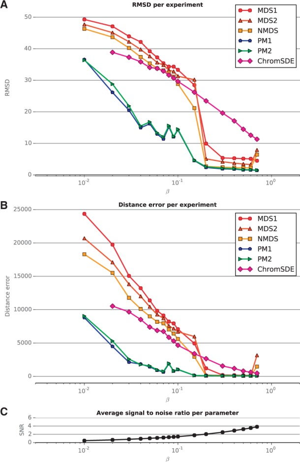
Performance evaluation on simulated data, varying the parameter β. (A) RMSD of each experiment for varying values of the parameter β. ChromSDE failed to yield consistent results for 14 experiments (it reported the wrong number of beads in the results file), and the PM2 algorithm failed to converge at the desired precision for one experiment (it exceeded the maximum number of iterations). (B) Distance error of each experiment for varying values of β. (C) Average SNR for each β. Higher SNR corresponds to better quality data

3.1.2 Metric versus non-metric methods: robustness to incorrect parameter estimation

Three of the methods tested, which we collectively refer to as metric methods, require as input a count-to-distance or distance-to-count transfer function: MDS1, MDS2 and PM1. In reality, however, the DNA may not follow the ideal physical laws underlying the default transfer function discussed in Section 2.4, and the structures inferred from these methods may diverge from the correct one because of miss-specification of the transfer function.

To assess this phenomenon, and evaluate the robustness of the different methods (including NMDS and PM2, which automatically infer a transfer function), we now study the performance of the methods on datasets generated with varying α parameters. We therefore run the MDS1, MDS2, NMDS, PM1 and PM2 methods on the second ensemble of simulated datasets. We provide the default transfer function to all metric methods, thus inducing a miss-specification for all simulated datasets with α ≠ −3.

Figure 2 shows the RMSD of each method, averaged over the datasets with different β, as a function of α. The performance curve of PM1, which is the best method when the data are simulated with the correct parameter α = −3, exhibits a characteristic U-shape centered around α = −3. This curve confirms that PM1 performs better when given the true parameter and performs worse as α moves away from −3. On the other hand, the performance curves of the two other metric methods, MDS1 and MDS2, do not exactly follow this trend: MDS1 and NMDS perform increasingly better when α decreases, and MDS2 achieves the best performance when α = −3.5. This phenomenon occurs because in our simulation, when α decreases, the SNR for a given β increases, counterbalancing the negative effect of the transfer function miss-specification. Thus, for MDS-based methods, it is apparently more important to have more data than to have a correct α parameter. Finally, we see that, as expected, the non-metric approaches, NMDS and PM2, are more robust to transfer function misspecification than the metric approaches because they automatically estimate it. When the parameter is wrong, PM2 outperforms the other methods for low SNR, whereas for high SNR, NMDS performs better.

Fig. 2.

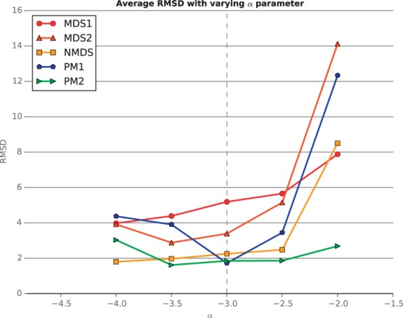
Performance evaluation for simulated data, varying the parameter α. The figure plots the average RMSD of the inferred structures for a range of α values. As α increases, the SNR of the dataset also increases

3.2 Real Hi-C data

We now test the different methods on real Hi-C data. Because in this case the true consensus structure is unknown, we investigate the behaviors of the different methods in terms of their ability to infer consistent structures from different datasets and across resolutions.

3.2.1 Stability to enzyme replicates

The Hi-C assay depends on a restriction enzyme to cleave the DNA after cross-linking, and the same sequence library can be analyzed multiple times using different enzymes. Although the resulting restriction fragments will differ, we expect a priori that the overall genome architecture should be the same from such replicate experiments. We therefore evaluate each genome architecture inference method with respect to the similarity of the structures inferred from two replicate Hi-C experiments that differ only in the choice of restriction enzyme. Specifically, we apply each method to two enzyme replicates, HindIII and NcoI, carried out in mouse embryonic stem (ES) cells (Dixon et al., 2012) for chromosomes 1–19.

To measure the stability of the methods, we compute (i) the Spearman correlation between the two pairwise Euclidean distance matrices of the pairs of predicted structures and (ii) the RMSD between the rescaled predicted structures. Note that, before computing our two error measures, we filter out from the pair of structures any beads for which the inference has not been done on either dataset, i.e. beads that have zero contact counts in either dataset.

To give a sense of how similar the two replicate datasets are, we also compute the Spearman correlation directly on the data, rather than on the inferred structures. As expected (Table 1), the higher the resolution is, the lower the correlation between the pairs of datasets is and the more different the inferred structures are. Across different enzyme replicates, the PM2 method yielded significantly higher correlation than all of the other methods (P < 0.05, signed-rank test adjusted for multiple tests with a Bonferroni correction).

Table 1.

Stability across enzyme replicates

Resolution	Corr	MDS1		MDS2		NMDS		PM1		PM2
		Corr	RMSD	Corr	RMSD	Corr	RMSD	Corr	RMSD	Corr	RMSD
1 Mb	0.981	13.13	0.945	5.54	0.964	5.80	0.965	7.28	0.931	4.92	0.976
500 kb	0.959	10.00	0.942	5.68	0.959	5.67	0.959	7.14	0.913	4.66	0.968
200 kb	0.845	5.64	0.940	3.74	0.945	3.73	0.946	4.01	0.891	3.42	0.958
100 kb	0.605	5.07	0.736	2.53	0.676	2.52	0.666	2.51	0.664	2.76	0.771

Note: For each resolution, the table lists the Spearman correlation the two enzyme replicate datasets, and, for each inference method, the average RMSD and Spearman correlation between pairs of structures inferred from the two datasets. Boldface values correspond to the best RMSD or correlation values among all five methods. In general, higher resolution leads to a lower correlation between pairs of inferred structures.

3.2.2 Stability to resolution

Zhang et al. (2012) show that the mapping from contact counts to physical distance differs from one resolution to another, underscoring the importance of good parameter estimation. To study the stability of the structure inference methods to changes in resolution, we compute the RMSD between pairs of structures inferred at different resolutions. Let $(X,Y)\in (R^{3\times n},R^{3\times m})$ be a pair of predicted structures such that n < m (i.e. X is a structure at a lower resolution than Y). We compute a downsampled structure $Y^{*}\in X^{3\times n}$ at the same resolution as X by averaging the coordinates of beads. We then compute the RMSD between this new structure Y* and X, as well as a corresponding Spearman correlation of the distance matrices.

Results are shown in Figure 3 and Table 2. PM2 is significantly (P < 0.05) more stable to resolution changes, both in terms of RMSD and correlation of distances.

Fig. 3.

Predicted structures for chromosome 1 at different resolution Contact counts matrices and predicted structures for the MDS2, NMDS, PM1 and PM2 methods at 1 Mb (A), 500 kb (B), 200 kb (C) and 100 kb (D)

Table 2.

Stability across resolution

Measure	MDS1	MDS2	NMDS	PM1	PM2
RMSD	14.86	12.92	12.98	13.03	11.48
Correlation	0.781	0.754	0.738	0.737	0.807

Note: The table lists the average RMSD and Spearman correlation between pairs of structures of different resolutions. In bold are the lowest average RMSD and highest average Spearman correlation. These values were computed on mouse ESC HindIII libraries [Dixon et al. (2012)].

4 DISCUSSION AND CONCLUSION

In this work, we present a novel method for inferring a consensus genomic 3D structure from Hi-C data. The method maximizes a likelihood derived from a statistical model of the relationship between the contact counts and physical distances, and includes an automatic tuning of the parameters defining the link between a 3D distance and the Poisson parameter of the corresponding contact count. We showed in simulations that the new method outperforms a panel of MDS-based approaches, including ChromSDE, which optimize an often ad hoc stress function. The improvement is particularly important at low SNR, corresponding to more difficult problems where we want to increase the resolution of the model with a fixed total number of reads; this is typically the situation where one expects a correct maximum likelihood estimator to outperform more ad hoc estimators. We also showed that misspecification in the count-to-distance transfer function can harm the performance of metric methods, while our model can adapt to unknown distributions within a parametric family. Finally, we also demonstrated, on real Hi-C data, the robustness of our methods to resolution change and enzyme duplicated datasets.

Our probabilistic model of reads is similar to the model proposed by Hu et al. (2013); however, instead of generating a family of structures by MCMC we use the model for direct maximum likelihood estimation of a consensus structure. Although the consensus structure might not be a definitive structure in vivo, it provides us with a rich model for further analysis, conserving hallmarks of genome organization such as the water lily form of the budding yeast (Duan et al., 2010) or topological domains (Kalhor et al., 2011).

The PM underlying our approach remains basic and could be subject to many improvements. For example, physical constraints, such as the size of the nucleus, could be incorporated into the model. Better models for zero entries may be possible because those can either come either from non-interacting loci or from measurement errors due to, for example, mappability problems. Overall, expressing the structure inference problem as a maximum likelihood problem offers a principled way to improve the method by improving the probabilistic model of measured data.

REFERENCES

- Ay F, et al. Statistical confidence estimation for Hi-C data reveals regulatory chromatin contacts. Genome Res. 2014a;113 doi: 10.1101/gr.160374.113. doi: 10.1101/gr.160374.113. [DOI] [PMC free article] [PubMed] [Google Scholar]
- Ay F, et al. Three-dimensional modeling of the P. falciparum genome during the erythrocytic cycle reveals a strong connection between genome architecture and gene expression. Genome Res. 2014b doi: 10.1101/gr.169417.113. doi: 10.1101/gr.169417.113. [DOI] [PMC free article] [PubMed] [Google Scholar]
- Bau D, et al. The three-dimensional folding of the α-globin gene domain reveals formation of chromatin globules. Nat. Struct. Mol. Biol. 2011;18:107–114. doi: 10.1038/nsmb.1936. [DOI] [PMC free article] [PubMed] [Google Scholar]
- Ben-Elazar S, et al. Spatial localization of co-regulated genes exceeds genomic gene clustering in the saccharomyces cerevisiae genome. Nucleic Acids Res. 2013;41:2191–2201. doi: 10.1093/nar/gks1360. [DOI] [PMC free article] [PubMed] [Google Scholar]
- Best MJ, et al. Minimizing separable convex functions subject to simple chain constraints. SIAM J. Optim. 1999;10:658–672. [Google Scholar]
- De S, Michor F. DNA replication timing and long-range DNA interactions predict mutational landscapes of cancer genomes. Nat. Biotechnol. 2011;29:1103–1108. doi: 10.1038/nbt.2030. [DOI] [PMC free article] [PubMed] [Google Scholar]
- Dekker J, et al. Capturing chromosome conformation. Science. 2002;295:1306–1311. doi: 10.1126/science.1067799. [DOI] [PubMed] [Google Scholar]
- Dixon JR, et al. Topological domains in mammalian genomes identified by analysis of chromatin interactions. Nature. 2012;485:376–380. doi: 10.1038/nature11082. [DOI] [PMC free article] [PubMed] [Google Scholar]
- Duan Z, et al. A three-dimensional model of the yeast genome. Nature. 2010;465:363–367. doi: 10.1038/nature08973. [DOI] [PMC free article] [PubMed] [Google Scholar]
- Fudenberg G, Mirny LA. Higher-order chromatin structure: bridging physics and biology. Curr. Opin. Genet. Dev. 2012;22:115–124. doi: 10.1016/j.gde.2012.01.006. [DOI] [PMC free article] [PubMed] [Google Scholar]
- Grosberg AY, et al. The role of topological constraints in the kinetics of collapse of macromolecules. J. Phys. 1988;49:2095–2100. [Google Scholar]
- Hu M, et al. Bayesian inference of spatial organizations of chromosomes. PLoS Comput. Biol. 2013;9:e1002893. doi: 10.1371/journal.pcbi.1002893. [DOI] [PMC free article] [PubMed] [Google Scholar]
- Imakaev M, et al. Iterative correction of Hi-C data reveals hallmarks of chromosome organization. Nat. Methods. 2012;9:999–1003. doi: 10.1038/nmeth.2148. [DOI] [PMC free article] [PubMed] [Google Scholar]
- Kalhor R, et al. Genome architectures revealed by tethered chromosome conformation capture and population-based modeling. Nat. Biotechnol. 2011;30:90–98. doi: 10.1038/nbt.2057. [DOI] [PMC free article] [PubMed] [Google Scholar]
- Kruskal J. Multidimensional scaling by optimizing goodness of fit to a nonmetric hypothesis. Psychometrika. 1964;29:1–27. [Google Scholar]
- Kruskal JB, Wish M. Multidimensional Scaling. Beverly Hills, CA: Sage Publications; 1977. [Google Scholar]
- Le TBK, et al. High-resolution mapping of the spatial organization of a bacterial chromosome. Science. 2013;342:731–734. doi: 10.1126/science.1242059. [DOI] [PMC free article] [PubMed] [Google Scholar]
- Lieberman-Aiden E, et al. Comprehensive mapping of long-range interactions reveals folding principles of the human genome. Science. 2009;326:289–293. doi: 10.1126/science.1181369. [DOI] [PMC free article] [PubMed] [Google Scholar]
- Nagano T, et al. Single-cell Hi-C reveals cell-to-cell variability in chromosome structure. Nature. 2013;502:59–64. doi: 10.1038/nature12593. [DOI] [PMC free article] [PubMed] [Google Scholar]
- Pedregosa F, et al. Scikit-learn: machine learning in Python. J. Mach. Learn. Res. 2011;12:2825–2830. [Google Scholar]
- Rousseau M, et al. Three-dimensional modeling of chromatin structure from interaction frequency data using Markov chain Monte Carlo sampling. BMC Bioinformatics. 2011;12:414. doi: 10.1186/1471-2105-12-414. [DOI] [PMC free article] [PubMed] [Google Scholar]
- Ryba T, et al. Evolutionarily conserved replication timing profiles predict long-range chromatin interactions and distinguish closely related cell types. Genome Res. 2010;20:761–770. doi: 10.1101/gr.099655.109. [DOI] [PMC free article] [PubMed] [Google Scholar]
- Shen Y, et al. A map of the cis-regulatory sequences in the mouse genome. Nature. 2012;488:116–120. doi: 10.1038/nature11243. [DOI] [PMC free article] [PubMed] [Google Scholar]
- Shepard R. The analysis of proximities: multidimensional scaling with an unknown distance function. i. Psychometrika. 1962;27:125–140. [Google Scholar]
- Tanizawa H, et al. Mapping of long-range associations throughout the fission yeast genome reveals global genome organization linked to transcriptional regulation. Nucleic Acids Res. 2010;38:8164–8177. doi: 10.1093/nar/gkq955. [DOI] [PMC free article] [PubMed] [Google Scholar]
- Tjong H, et al. Physical tethering and volume exclusion determine higher-order genome organization in budding yeast. Genome Res. 2012;22:1295–1305. doi: 10.1101/gr.129437.111. [DOI] [PMC free article] [PubMed] [Google Scholar]
- van Steensel B, Dekker J. Genomics tools for the unraveling of chromosome architecture. Nat. Biotechnol. 2010;28:1089–1095. doi: 10.1038/nbt.1680. [DOI] [PMC free article] [PubMed] [Google Scholar]
- Wächter A, Biegler LT. On the implementation of an interior-point filter line-search algorithm for large-scale nonlinear programming. Math Program. 2006;106:25–57. [Google Scholar]
- Yaffe E, Tanay A. Probabilistic modeling of Hi-C contact maps eliminates systematic biases to characterize global chromosomal architecture. Nat. Genet. 2011;43:1059–1065. doi: 10.1038/ng.947. [DOI] [PubMed] [Google Scholar]
- Zhang Y, et al. Spatial organization of the mouse genome and its role in recurrent chromosomal translocations. Cell. 2012;148:1–14. doi: 10.1016/j.cell.2012.02.002. [DOI] [PMC free article] [PubMed] [Google Scholar]
- Zhang Z, et al. Inference of spatial organizations of chromosomes using semi-definite embedding approach and Hi-C data. In: Deng M, et al., editors. 2013. Proceedings of the 17th International Conference on Research in Computational Molecular Biology, Vol. 7821 of Lecture Notes in Computer Science. Springer, Berlin, Heidelberg, pp. 317–332. [Google Scholar]