

Abstract
Previously, we reported development of a fast polarizable force field and software named POSSIM (POlarizable Simulations with Second order Interaction Model). The second-order approximation permits the speed up of the polarizable component of the calculations by ca. an order of magnitude. We have now expanded the POSSIM framework to include a complete polarizable force field for proteins. Most of the parameter fitting was done to high-level quantum mechanical data. Conformational geometries and energies for dipeptides have been reproduced within average errors of ca. 0.5 kcal/mol for energies of the conformers (for the electrostatically neutral residues) and 9.7° for key dihedral angles. We have also validated this force field by running Monte Carlo simulations of collagen-like proteins in water. The resulting geometries were within 0.94 Å root-mean-square deviation (RMSD) from the experimental data. We have performed additional validation by studying conformational properties of three oligopeptides relevant in the context of N-glycoprotein secondary structure. These systems have been previously studied with combined experimental and computational methods, and both POSSIM and benchmark OPLS-AA simulations that we carried out produced geometries within ca. 0.9 Å RMSD of the literature structures. Thus, the performance of POSSIM in reproducing the structures is comparable with that of the widely used OPLS-AA force field. Furthermore, our fitting of the force field parameters for peptides and proteins has been streamlined compared with the previous generation of the complete polarizable force field and relied more on transferability of parameters for nonbonded interactions (including the electrostatic component). The resulting deviations from the quantum mechanical data are similar to those achieved with the previous generation; thus, the technique is robust, and the parameters are transferable. At the same time, the number of parameters used in this work was noticeably smaller than that of the previous generation of our complete polarizable force field for proteins; thus, the transferability of this set can be expected to be greater, and the danger of force field fitting artifacts is lower. Therefore, we believe that this force field can be successfully applied in a wide variety of applications to proteins and protein–ligand complexes.
I. Introduction
Computer simulations have become invaluable in biophysical research. Quantum mechanical calculations can yield very valuable data in many applications, but the area of their utility is still limited. Therefore, employing empirical force fields remains the method of choice in the majority of computational biophysical projects.
Accurate calculations with empirical force fields often require that explicit treatment of electrostatic polarization would be included.1−4 Examples of such cases include small molecule and protein pKa assessments as well as accurate calculations of binding energies, especially those of ions. We have previously demonstrated that using a polarizable force field allows us to reduce the errors in calculating pKa values of the acidic residues of the OMTKY3 protein from 3.3 to 0.6 pH units,2a and from 2.1 to 0.7 pH units for the basic residues.2b We have also showed that polarization is required for predicting a thermodynamically stable structure for the complex of the CopZ protein with the Cu(I) ion.4
Therefore, polarization is a crucial component in many computational studies of proteins and protein–ligand complexes. In some cases, it is included in surrogate forms, such as conformation-specific protein charges.5
Some prominent examples of the development and use of polarizable force fields include the following. MacKerell and Roux have developed and applied a polarization model based on the classical Drude oscillator. In this case, the polarization is represented by a charge with a fictitious mass that can move away from its original position at an atomic center.6a The Drude oscillator model has also been used with the CHARMM force field.6b,6c The AMOEBA polarizable force field included in the TINKER computational package has been developed by Ponder and co-workers. It has been successfully used in a number of applications from modeling of small molecules to protein–ligand binding calculations.6d SIBFA polarizable methodology has been employed in simulations of ion binding in metalloproteins and hydrated metal ion systems.6e Explicit polarization can be used with AMBER.6f
At the same time, there are still unresolved issues with polarizable force fields, which prevents them from being employed in an even broader range of applications. First, functional forms used in polarizable simulations vary significantly. Inducible point dipole, fluctuating charges, point multipoles, the Drude oscillator, and continuum dielectric models are all employed in such simulations. While it is certainly good to have a variety of tools available, it would also be beneficial to have a better analysis as to what are their relative advantages in various areas of application.
Second, polarizable calculations are more time-consuming than nonpolarizable ones. While polarizable calculations can have low overhead when systems such as pure simple liquids are considered and the tools are optimized for such tasks, if a computational framework has to be able to deal with a variety of chemically and biologically relevant systems, the overhead grows significantly.
Third, parametrizing a polarizable force field permits one to use more parameters than for fixed-charges force fields, and thus arises the issues of overparameterization and transferability. Ideally, a polarizable force field should have relatively few new parameters, their values should be as standardized across the set of test and target molecular systems as possible, and the parameters should be as transferable from small to large molecules as practical. Such transferability should ensure that the resulting force field would work well in new applications and environments without additional refitting.
Finally, there is the issue of choosing the source of the fitting target data. High-level quantum mechanical calculations can be very useful, but we have demonstrated that they have to be significantly supplemented by experimental data.7,8 Overall, we have been pursuing a balanced approach of using both quantum mechanical and experimental results in building fitting target for force field development.
We have implemented a second-order approximation to the inducible point dipole approximation that permits the speed up of polarizable calculations by ca. an order of magnitude without any loss of accuracy.9,10 This method also eliminated the danger of the so-called polarization catastrophe (the resonance-like infinite growth of the induced dipole moment values). The resulting software and force field of the POSSIM framework is used in simulations described in this article.
We have also pursued the goal of transferability and significantly reduced the number of parameters fitted in the presented complete polarizable force field for proteins, as compared to those employed in the previous generation of polarizable protein force field.7 This should even further strengthen the ability of the polarizable force field to reproduce and predict molecular properties in various environments based on the physically correct underlying basis rather than on parametrization to specific circumstances.
Previously, we successfully developed polarizable POSSIM parameters for a number of small molecules10 and alanine and protein backbones,11 as well as the lysine residue.12 Following this success, we have now extended the development of the POSSIM force field to the complete set of amino acids and applied it in test simulations of a collagen-like protein. The results are presented in this article.
One of the validations that we performed were by conformational studies of three oligopeptides related to the issue of secondary structure of N-linked glycoproteins: Ac-NGS-NHBn and two of its mutated forms, Ac-QGS-NHBn and Ac-NPS-NHBn. These systems have been previously studied by combined experimental and computational means,13 and thus, the geometry of four stable conformers of each of them has been determined. It was shown that the changes in the residues introduced in the mutated forms have a significant influence on the secondary structure properties of the motif,13 and thus, the ability of force fields to reproduce structures of these molecules is important. We have simulated the 12 systems (four conformers for each of the three peptides) with both POSSIM and fixed-charges OPLS-AA force fields. The latter is known to provide a reliable framework for modeling protein structure, and thus, using it as a benchmark was justified as a means of validating the reported POSSIM parameters.
The rest of the paper is organized as follows: Given in Section II is a description of the methodology involved. Section III contains results and discussion. Finally, conclusions are presented.
II. Methods
A. Force Field
In the POSSIM force field, the total energy Etot is calculated by adding the electrostatic interactions Eelectrostatic, the van-der-Waals energy EvdW, harmonic bond stretching and angle bending Estretch and Ebend, and the torsional energy Etorsion terms:
| 1 |
The electrostatic polarization is manifested via inducible point dipoles μ:
| 2 |
Here E0 is the electrostatic field in the absence of the induced dipoles. Then,
| 3 |
where α stands for the scalar polarizabilities and Tij is the dipole–dipole interaction tensor. The typical way of solving eq 3 for large molecular systems is by applying iterations in order to reach self-consistency. The first two iterations in this procedure are
| 4a |
| 4b |
The fast polarization technique employed in the POSSIM formalism uses the second-order expression in eq 4b. We have previously shown that it yields an increase in computational speed compared to the full-convergence polarizability formalism without loss of accuracy.9,10 In addition, the POSSIM force field also contains a pairwise-additive contribution from interactions of the fixed charges:
| 5 |
where the factor fij is set to zero for 1,2- and 1,3-pairs (atoms which belong to the same valence bond or angle respectively), to 0.5 for 1,4-interactions (atoms in the same dihedral angle), and to 1.0 for all other pairs.
POSSIM also utilizes a short-distance cutoff parameter Rcut = 0.8 Å. If the distance between two atoms Rij is smaller than the sum of these parameters Rminij = Rcuti + Rcutj for the atoms i and j, Rij is replaced by a smoothing function:
| 6 |
The approximation in eq 4b differs from the exact physical induced-dipole electrostatic model, but it also increases the computational speed without compromising the accuracy of the simulations.9,10 The second-order formalism also turns the expression for the inducible dipoles into an analytical one, and the possibility of the polarization catastrophe is fundamentally eliminated. This feature of truncated self-consistency is also useful in extending this methodology to building continuum solvation models, since it removes the convergence issue—a potential problem in the creation and parametrization of such methods.
The POSSIM force field uses the standard Lennard-Jones formalism for the van-der-Waals energy:
 |
7 |
Geometric combining rules are applied as εij = (εiεj)1/2, σij = (σiσj)1/2. Harmonic bond stretching and angle bending potentials were used. The torsional term is obtained as the following Fourier series:
| 8 |
All the POSSIM stretch and bend parameters were adopted from the OPLS-AA force field without any change, while the torsional parameters were either fitted previously10,11 or produced in the course of this project.
B. Parameterization of the Complete Protein Force Field
In the overwhelming majority of the cases, small molecule analogues of the side chains had been parametrized previously.14 In these instances, parametrization consisted of fitting torsional parameters for the χ1, χ2, etc. dihedrals of the side chains. The backbone parameters, including the ϕ and ψ torsions, were taken directly from the alanine dipeptide set.11
It should be specifically emphasized that, unlike in the process of producing the previous generation of the polarizable force field for proteins (PFF),7 we did not refit parameters for nonbonded interactions for the residues but adopted them from the corresponding small molecules without any change. For example, methanol parameters were used in serine, acetamide in asparagine and glutamine, etc. The performance of the resulting POSSIM force field is no less accurate than that of the previously parametrized PFF, as will be shown in the Results section. Therefore, we conclude that the transferability of the POSSIM formalism and parameters is excellent and that the quality of the POSSIM framework does not suffer from overparameterization or excessive requirements and complexity in the parametrization process.
A brief summary of the torsional fitting technique is as follows: (i) Side-chain torsions were fit for CH3–capped dipeptides. (ii) The fitting was done with ab initio data as the target. Unless otherwise noted, we used results of LMP2/cc-pVTZ(-f)//HF-6-31G** calculations7,8 carried out with the Jaguar software suite.15 (iii) The fitting subspace for any coupled torsions (such as χ1 and χ2) in side-chains consisted of the point of the quantum mechanical energy minimum and four additional points in each direction with 20° spacing, for a total of 17 points for two-dimensional coupled torsions for each minimum. This was the same choice of the fitting subspace as we applied in protein force field fitting projects before. For charged residues, the minima were found in continuum aqueous solution, but the actual energies of the rotamers were calculated in the gas phase (for comparison with the POSSIM results) with all the ϕ, ψ, and side-chain χ dihedral values fixed. In case of electrostatically neutral residues, the backbone dihedral values were allowed to change, and all the simulations were carried out in vacuum. (iv) The resulting parameters were tested by reproducing the quantum mechanical conformational energies and geometries of the capped dipeptides. (v) Initial guesses for the torsional parameters were found by applying a non-Boltzmann weighting scheme for the error at the fitting points:
| 9 |
Here, Gi stands for the absolute value of the torsional surface gradient at point i, for which the weight Wi is to be produced. The coefficient A is adjusted to change the maximum to minimum weight ratio for the fitting and is chosen independently for each particular dipeptide fitting. The parameters were then further adjusted to minimize errors in the conformational energies and dihedral angles.
For two of the residues, arginine and tryptophan, additional fitting of the corresponding small molecule analogues of the side-chains had to be done first. The methodology employed for arginine was similar to that used in fitting the lysine residue.12 We fitted values of the atomic polarizabilities to reproduce three-body energies of the methylguanidinium cation14 (the arginine side-chain analogue) with two dipolar probes. The values of the nonbonded parameters were then derived to yield gas-phase dimerization energies for the cation with one water molecule in agreement with the extrapolated16 LMP2/cc-pVTZ(-f)–LMP2/cc-pVQZ(-g) energies. Torsional parameters were chosen to reproduce LMP2/cc-pVTZ(-f) profiles. After that, parameters for the methylguanidinium molecule were employed in torsional fitting for the arginine residue in the way described above for the charged amino acids.
In order to produce the side-chain analogue for tryptophan, we first determined values of the parameters for pyrrole. The procedure was similar to that used for methylguanidinium above, except that liquid pyrrole was simulated as well. 216 molecules were simulated at 25 °C and 1 atm with our POSSIM software10 using the Monte Carlo technique in an NPT ensemble. Nonbonded cutoffs for dipole–dipole interactions were set at 7 Å, and all the other nonbonded cutoffs were set at 11 Å. The usual term for correcting the Lennard-Jones energy for employing the cutoff was used. Our goal was to adjust parameters to reproduce the heat of vaporization and density of liquid pyrrole. The indole analogue of the tryptophan side chain was built by pasting together parameters for the pyrrole molecule and the standard POSSIM parameters for benzene14 for the remaining part of the aromatic system. The torsional fitting for tryptophan was carried out in the same way as for the other electrostatically neutral residues.
It should also be pointed out that this version of our complete polarizable force field for proteins (POSSIM) contains fewer parameters than the previous one (PFF7). For example, virtual sites are not used on oxygen atoms or at the middle of C–H bonds, van-der-Waals interactions are described by only two terms, and permanent dipoles are not used. Thus, one can expect that the probability of encountering anomalous simulation results due to artifacts of parameter fitting with POSSIM should be lower.
C. Simulations of the Collagen-Like Peptide
We simulated a collagen-like peptide trimer (PDB ID 3AH9) as a test case. Simulations were carried out with POSSIM, using the Monte Carlo technique. The trimer is shown in Figure 1.
Figure 1.
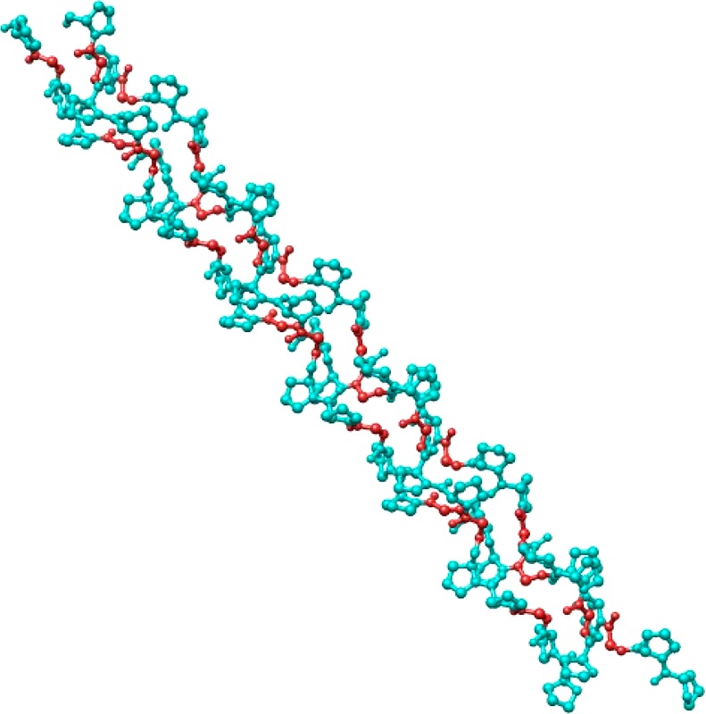
Collagen-like peptide trimer, PDB ID 3AH9.17
The system was solvated in 1000 water molecules in a periodic box of ca. 21.7 Å × 21.7 Å × 86.6 Å size. We employed NPT simulations at 25 °C and 1 atm. Overall, 13 × 106 Monte Carlo configurations were used. The root-mean-square deviation (RMSD) from the X-ray PDB structure was determined as a measure of adequacy of the POSSIM results.
D. Simulations of the Ac-NGS-NHBn, Ac-QGS-NHBn, and Ac-NPS-NHBn Peptides
We simulated these peptides with the POSSIM software. The system was modeled with gas-phase geometry optimizations of four conformers for each of the peptides, and the initial coordinates were taken from ref (13). Both second-order polarizable POSSIM and fixed-charges OPLS-AA force fields were employed. We compared geometries of the final structures to those from the combined experimental and theoretical studies in ref (13) and the RMSDs are reported in the Results and Discussion section below.
III. Results and Discussion
A. Fitting Parameters for Methylguanidinium and Pyrrole
The methylguanidinium ion is an analogue of the arginine residue side-chain. Initial fitting of its parameters was done previously,14 but we have refined them in this work. There were seven possible hydrogen-bonded dipolar probe locations for this system.
Pairs of these probes were used in calculating three-body energies, and values of atomic polarizabilities were fitted to reproduce these three-body energy values. Five of the probes have their negative charges pointed toward the five polar hydrogen atoms of the cation. The other two have their positive point charges at hydrogen bonding distances from the −NH2 nitrogens, as can be seen from Figure 2. Therefore, there is a total of twenty-one possible three-body energies for the methylguanidinium cation. The average absolute error in the three-body energies of methylguanidinium was only 0.118 kcal/mol, which is a great result given that there are 21 three-body values.
Figure 2.
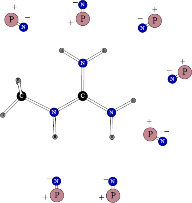
Dipolar probes used in calculating three-body energy of the methyl guanidinium ion. Symbols “P” and “N” denote the positive and negative point charges, respectively.
The only dimer considered for this ion is shown in Figure 3. The planes of the water molecule and methylguanidinium are perpendicular to each other. The position of the water molecule is almost completely symmetric with respect to the nitrogen atoms but with a ca. 0.1 Å shift toward the nitrogen connected to the methyl group. The quantum mechanical dimerization energy is −17.86 kcal/mol, and the distances between the nitrogen atoms and the water oxygen are 2.98 and 3.09 Å. Our refitting of the N–H charge distribution and the Lennard-Jones σ parameter for nitrogen produced a dimerization energy of −17.19 kcal/mol and nitrogen–oxygen distances of 2.92 and 3.04 Å.
Figure 3.
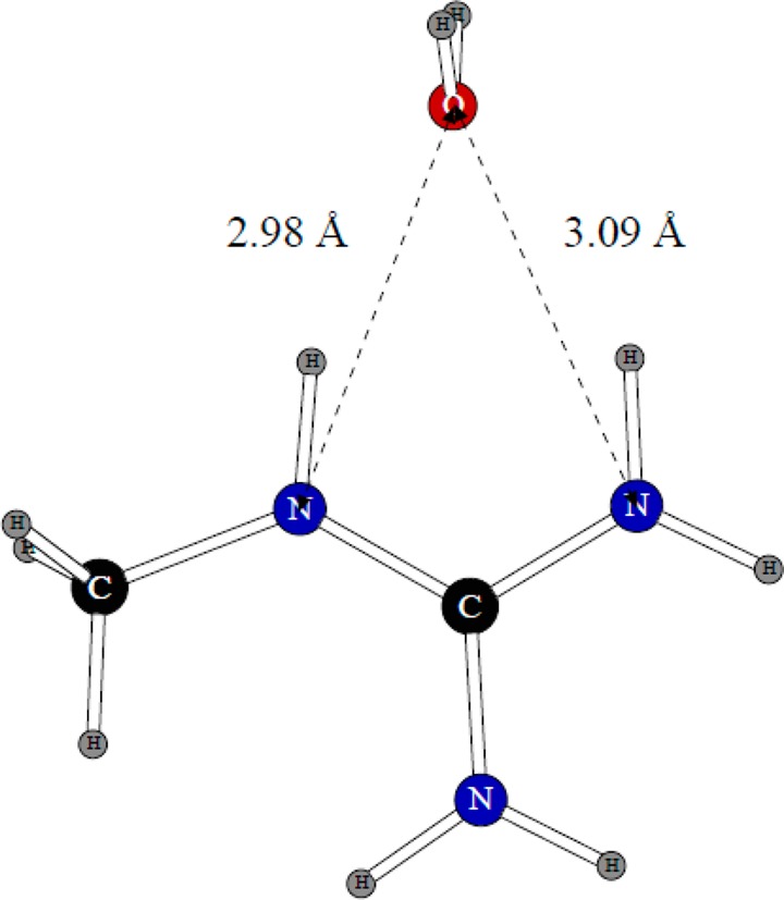
Dimer of the methylguanidinium ion with one water molecule.
Results of the torsional fitting are presented in Table 1. The average error in torsional energy is 0.099 kcal/mol and the largest single error is 0.333 kcal/mol.
Table 1. Torsional Energies for Methylguanidinium and Pyrrole (kcal/mol).
| molecule | dihedral | angle values (deg) | energy, QMa | energy, POSSIM |
|---|---|---|---|---|
| C2N3H8+ | H–N(H2)–C–N | 0 | 0.000 | –0.333 |
| 30 | 0.175 | 0.482 | ||
| 60 | 2.615 | 2.641 | ||
| C–N–C–N(H2) | 0 | 0.000 | –0.097 | |
| 15 | 0.140 | 0.217 | ||
| 30 | 1.115 | 1.136 | ||
| H–C(sp3)–N–C | 0 | 1.191 | 1.176 | |
| 60 | 0.000 | 0.008 | ||
| 180 | 0.000 | 0.008 | ||
| C4NH5 | H–N–C–C | 180 | 0.000 | –0.001 |
| 165 | 0.424 | 0.438 | ||
| 150 | 1.345 | 1.432 |
LMP2/cc-pVTZ(-f).
The pyrrole molecule was fused with a benzene ring to produce the POSSIM model for the tryptophan residue. There are three dipolar probes used in three-body energy fitting, as shown in Figure 4.
Figure 4.
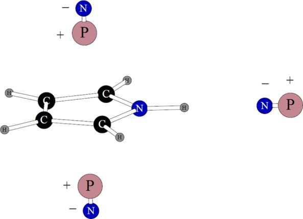
Dipolar probes used in calculating three-body energy of pyrrole. Symbols “P” and “N” denote the positive and negative point charges, respectively.
We did fitting only for the nitrogen polarizability, the polar hydrogen had no polarizability associated with it, and the other atoms had their parameters adopted from benzene POSSIM.14 The average unsigned error of the three calculated three-body energies for pyrrole was 0.184 kcal/mol.
The dimer with water employed in fitting the nonbonded parameters is shown in Figure 5.
Figure 5.
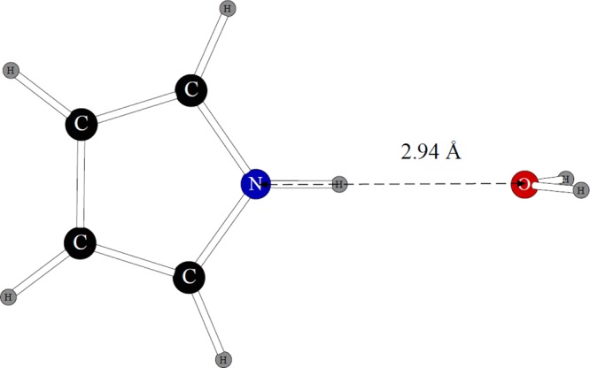
Dimer of pyrrole with one water molecule.
We adjusted only the nitrogen Lennard-Jones parameters and the N–H electrostatic charge separation. Once again, the rest of the atoms had their parameters taken directly from the benzene model. The quantum mechanical distance between the oxygen and nitrogen atoms was 2.94 Å, and the dimerization energy is −5.13 kcal/mol. The POSSIM results are 3.03 Å and −5.71 kcal/mol. Thus, the geometry is reasonably close to the ab initio data, with the distance being within 0.1 Å error, and the energy is 0.58 kcal/mol, which is within the error range that was observed for dimers containing water molecules previously.10
Torsional fitting for the pyrrole molecule involved adjusting the V2 coefficient in eq 8 for the H–N–C–C torsion (V1 and V3 for this angle were kept constant and zero). It can be seen from the results presented in Table 1 that the agreement with the quantum mechanical data is very good, and the average error is only 0.009 kcal/mol.
Since pyrrole is an electrostatically neutral molecule, we could also run pure liquid pyrrole simulations to assess the enthalpy of vaporization and molecular volume at 25 °C. The results of these POSSIM simulations were ΔHvap = 10.60 kcal/mol and V = 117.4 Å3. The experimentally determined values are 10.80 kcal/mol and 115.3 Å3, respectively.18 Thus, the error in the heat of vaporization is 1.9% and in the molecular volume (and thus in density) is 1.8%; both numbers are in good agreement with the experimental data.
With the creation of the parameter sets for pyrrole and the methylguanidinium ion, we have all the potential energy parameters of the small molecule analogs needed for fitting models of the protein residues.
B. Parameterization of Protein Residues
Alanine and Lysine
Parameters for the alanine11 and lysine12 residues were produced previously. We did not refit them in this work.
Other Residues
Results of applying the produced torsional parameters for serine, phenylalanine, cysteine, asparagine, glutamine, protonated and deprotonated histidine, leucine, isoleucine, valine, methionine, proline, tryptophan, threonine, tyrosine, protonated and deprotonated aspartic and glutamic acids, and arginine are presented in Tables 2–22. Overall, the performance of POSSIM is robust. Given in Table 23 is comparison of the energy and dihedral angle deviations from the quantum mechanical targets for POSSIM, OPLS-AA, and PFF (the previously developed polarizable force field).7 The average deviations with all three techniques are almost completely the same, with the energy and key dihedral angle errors for the neutral residues being ca. 0.5 kcal/mol and 10°, respectively. Thus, we conclude that the POSSIM methodology is adequate for reproducing these properties. It should also be emphasized that the POSSIM errors are about the same as the PFF ones, even though the number of parameters in the latter is greater.
Table 2. Conformational Energies (kcal/mol) and Angles (deg) for Serine Dipeptidea.
| energy |
ϕ |
ψ |
χ1 |
χ2 |
||||||
|---|---|---|---|---|---|---|---|---|---|---|
| conf. | QM | P | QM | P | QM | P | QM | P | QM | P |
| 1 | 0.00 | –0.32 | –85.4 | –75.0 | 75.0 | 35.5 | 54.1 | 63.5 | 67.3 | 70.2 |
| 2 | 2.76 | 2.86 | –157.5 | –166.2 | –176.10 | 178.0 | –166.10 | –162.9 | 82.5 | 82.5 |
| 3 | 3.75 | 3.65 | –156.7 | –165.5 | 178.5 | 169.8 | –170.7 | –170.6 | 167.9 | 168.0 |
| 4 | 3.95 | 3.92 | –171.5 | –163.9 | 166.2 | 157.0 | –92.9 | –92.1 | 53.9 | 53.7 |
| 5 | 5.12 | 5.25 | –154.3 | –158.0 | 174.2 | 169.3 | 66.1 | 81.6 | –61.2 | –61.3 |
| 6 | 7.43 | 7.65 | –157.7 | –157.5 | 172.5 | 172.8 | 68.0 | 75.5 | –167.5 | –170.6 |
| error | 0.19 | 6.6 | 11.4 | 6.1 | 1.1 | |||||
QM stands for the quantum mechanical data (from ref (7)); P stands for POSSIM results from this work.
Table 22. Conformational Energies (kcal/mol) for Arginine Dipeptidea.
| energy |
||
|---|---|---|
| conformer | QM | POSSIM |
| 1 | 0.00 | 0.00 |
| 2 | 10.76 | 10.73 |
| 3 | 3.29 | 3.28 |
| 4 | 13.87 | 19.97 |
| 5 | 8.58 | 8.65 |
| 6 | 4.25 | 4.19 |
| error | 1.05 | |
QM stands for the quantum mechanical data (from ref (7)); POSSIM results are from this work.
Table 23. Average Conformational Energy (kcal/mol) and Dihedral Angle (deg) Deviations from the Quantum Mechanical Results for POSSIM As Well As for OPLS and PFF (Previously Developed Polarizable Force Field)a.
| POSSIM |
OPLS-AA |
PFF |
||||
|---|---|---|---|---|---|---|
| residue | energy | angles | energy | angles | energy | angles |
| serine | 0.19 | 6.3 | 0.34 | 4.9 | 0.34 | 8.1 |
| phenylalanine | 0.02 | 8.9 | 0.15 | 7.5 | 0.02 | 9.5 |
| cysteine | 0.25 | 6.0 | 0.35 | 5.8 | 0.27 | 4.8 |
| asparagine | 0.14 | 8.6 | 0.16 | 19.5 | 0.02 | 8.7 |
| glutamine | 0.58 | 16.3 | 0.96 | 13.9 | 0.92 | 18.0 |
| Hid | 0.94 | 15.6 | ||||
| Hie | 0.68 | 8.7 | 0.85 | 18.7 | 0.83 | 18.2 |
| leucine | 1.02 | 5.4 | 0.35 | 5.9 | 0.35 | 5.1 |
| isoleucine | 0.54 | 6.7 | 0.38 | 5.5 | 0.88 | 11.8 |
| valine | 0.13 | 5.1 | 0.08 | 8.4 | 0.01 | 5.1 |
| methionine | 0.23 | 5.1 | 0.59 | 5.2 | 0.53 | 5.4 |
| proline | 0.74 | 1.54 | 1.27 | |||
| tryptophan | 0.75 | 19.2 | 0.50 | 24.2 | 0.49 | 19.4 |
| threonine | 0.76 | 6.9 | 0.87 | 6.9 | 0.75 | 8.9 |
| tyrosine | 0.27 | 13.7 | 0.39 | 8.1 | 0.27 | 8.9 |
| protonated Asp | 0.26 | 12.4 | ||||
| protonated Glu | 0.92 | 9.9 | ||||
| aspartic acid | 0.71 | 0.16 | 0.77 | |||
| glutamic acid | 1.48 | 1.53 | 1.47 | |||
| protonated His | <0.01 | 0.97 | 0.97 | |||
| arginine | 1.05 | 1.15 | 0.79 | |||
| avg. deviations | 0.48b/0.81c | 9.7b | 0.46b/0.95c | 10.3b | 0.44b/1.00c | 10.1b |
The OPLS and PFF results are from ref (7).
Electrostatically neutral residues, proline not included.
Charged residues.
Table 3. Conformational Energies (kcal/mol) and Angles (deg) for Phenylalanine Dipeptidea.
| energy |
ϕ |
ψ |
χ1 |
χ2 |
||||||
|---|---|---|---|---|---|---|---|---|---|---|
| conf. | QM | P | QM | P | QM | P | QM | P | QM | P |
| 1 | 0.00 | 0.02 | –156.1 | –160.2 | 150.2 | 160.8 | –171.7 | –160.1 | 72.4 | 71.1 |
| 2 | 0.88 | 0.86 | –88.7 | –73.6 | 76.7 | 36.2 | –57.6 | –59.6 | 112.0 | 119.4 |
| 3 | 1.65 | 1.64 | –157.7 | –160.4 | 166.1 | 162.6 | 55.8 | 55.9 | 85.7 | 78.2 |
| error | 0.02 | 7.3 | 18.2 | 4.6 | 5.4 | |||||
QM stands for the quantum mechanical data (from ref (7)); P stands for POSSIM results from this work.
Table 4. Conformational Energies (kcal/mol) and Angles (deg) for Cysteine Dipeptidea.
| energy |
ϕ |
ψ |
χ1 |
χ2 |
||||||
|---|---|---|---|---|---|---|---|---|---|---|
| conf. | QM | P | QM | P | QM | P | QM | P | QM | P |
| 1 | 0.00 | –0.38 | –86.6 | –74.1 | 64.7 | 34.2 | 52.4 | 63.3 | 68.1 | 64.7 |
| 2 | 1.72 | 1.77 | –159.2 | –157.8 | 166.7 | 160.4 | –160.7 | –160.6 | 75.4 | 73.8 |
| 3 | 2.26 | 2.20 | –156.8 | –156.9 | 144.1 | 144.0 | –174.8 | 179.9 | –81.4 | –71.2 |
| 4 | 3.18 | 3.50 | –154.8 | –156.4 | 174.4 | 163.6 | 65.1 | 69.2 | –65.1 | –53.9 |
| 5 | 4.79 | 4.86 | –160.0 | –175.3 | 166.1 | 165.1 | 62.8 | 65.4 | –175.3 | –176.2 |
| error | 0.25 | 3.9 | 9.8 | 4.6 | 5.5 | |||||
QM stands for the quantum mechanical data (from ref (7)); P stands for POSSIM results from this work.
Table 5. Conformational Energies (kcal/mol) and Angles (deg) for Asparagine Dipeptidea.
| energy |
ϕ |
ψ |
χ1 |
χ2 |
||||||
|---|---|---|---|---|---|---|---|---|---|---|
| conf. | QM | P | QM | P | QM | P | QM | P | QM | P |
| 1 | 0.00 | 0.10 | –166.3 | –168.3 | –176.1 | 172.4 | –138.7 | –133.7 | 89.3 | 88.4 |
| 2 | 3.49 | 3.38 | –179.2 | 176.7 | –135.3 | –102.1 | 55.3 | 48.7 | –99.4 | –94.1 |
| error | 0.14 | 3.0 | 22.3 | 5.8 | 3.1 | |||||
QM stands for the quantum mechanical data (from ref (7)); P stands for POSSIM results from this work.
Table 6. Conformational Energies (kcal/mol) and Angles (deg) for Glutamine Dipeptidea.
| energy |
ϕ |
ψ |
χ1/χ2/χ3 |
|||||
|---|---|---|---|---|---|---|---|---|
| QM | P | QM | P | QM | P | QM | P | |
| 1 | 0.19 | 0.40 | –154.1 | –157.9 | 167.6 | 163.0 | –99.6/–66.8/171.8 | –103.8/–53.9/148.1 |
| 2 | 0.46 | 0.62 | –146.1 | –152.5 | 169.2 | 158.9 | –84.1/–60.8/128.8 | –83.5/–52.9/123.9 |
| 3 | 0.00 | –0.65 | –158.8 | –156.7 | 154.2 | 148.1 | –174.7/54.0/89.9 | 154.9/66.4/163.9 |
| 4 | 1.07 | 1.68 | –84.9 | –76.6 | 57.1 | 32.1 | 66.3/–86.5/–155.8 | 70.5/–19.0/108.4 |
| 5 | 0.92 | 1.68 | –85.4 | –76.7 | 77.8 | 32.1 | 76.8/–48.5/126.7 | 70.4/–19.0/108.4 |
| 6 | 1.80 | 1.98 | –85.8 | –72.9 | 71.0 | 26.9 | –60.8/88.8/169.4 | –40.2/85.1/108.4 |
| 7 | 2.83 | 1.63 | –155.7 | –156.1 | 154.7 | 156.8 | 62.3/81.2/–154.4 | 80.8/78.1/163.1 |
| 8 | 4.02 | 4.32 | –86.5 | –79.3 | 78.0 | 67.0 | –174.6/172.8/150.6 | –175.2/–132.8/–137.9 |
| 9 | 5.29 | 4.76 | –138.7 | –150.5 | 160.9 | 153.1 | –62.3/–172.4/–170.0 | –50.8/–174.7/–179.2 |
| 10 | 5.32 | 5.43 | –153.6 | –162.1 | 164.6 | 160.6 | 59.0/171.6/150.5 | 63.1/166.1/152.9 |
| 11 | 8.54 | 8.60 | –153.4 | –151.7 | 166.7 | 160.0 | 38.6/54.2/62.5 | 39.5/37.7/82.8 |
| error | 0.58 | 6.5 | 14.6 | 9.3/19.6/31.6 | ||||
QM stands for the quantum mechanical data (from ref (7)); P stands for POSSIM results from this work.
Table 7. Conformational Energies (kcal/mol) and Angles (deg) for Hid Dipeptidea.
| energy |
ϕ |
ψ |
χ1 |
χ2 |
||||||
|---|---|---|---|---|---|---|---|---|---|---|
| conf. | QM | P | QM | P | QM | P | QM | P | QM | P |
| 1 | 4.69 | 2.90 | –82.7 | –72.8 | 68.1 | 22.5 | 44.6 | 45.2 | –120.8 | –90.4 |
| 2 | 3.59 | 4.74 | 177.9 | –163.0 | 168.1 | 155.4 | 38.8 | 41.1 | –94.8 | –83.0 |
| 3 | 3.02 | 3.06 | –161.4 | –161.1 | 132.9 | 148.8 | 173.2 | 176.3 | –86.9 | –79.1 |
| 4 | 0.00 | –0.27 | –163.5 | –163.1 | 173.0 | 157.5 | –132.5 | –123.1 | 65.7 | 62.7 |
| 5 | 3.46 | 3.40 | –87.2 | –74.6 | 70.7 | 30.1 | –51.4 | –43.5 | –66.0 | –60.8 |
| 6 | 6.74 | 6.82 | –114.1 | –74.5 | 144.3 | 36.6 | –62.6 | –60.6 | 162.5 | 162.4 |
| 7 | 2.64 | 3.49 | –169.9 | –159.5 | 136.7 | 150.5 | 40.1 | 49.4 | 58.9 | 48.4 |
| error | 0.94 | 13.2 | 34.6 | 4.9 | 9.8 | |||||
QM stands for the quantum mechanical data (from ref (7)); P stands for POSSIM results from this work.
Table 8. Conformational Energies (kcal/mol) and Angles (deg) for Hie Dipeptidea.
| energy |
ϕ |
ψ |
χ1 |
χ2 |
||||||
|---|---|---|---|---|---|---|---|---|---|---|
| conf. | QM | P | QM | P | QM | P | QM | P | QM | P |
| 1 | 0.00 | –0.44 | –85.2 | –70.2 | 48.0 | 18.0 | 56.3 | 59.3 | –74.8 | –82.3 |
| 2 | 0.19 | 0.18 | –162,3 | –164.7 | –178.3 | 175.1 | –143.1 | –145.1 | –67.3 | –78.3 |
| 3 | 2.41 | 2.52 | –154.0 | –164.2 | 149.8 | 157.9 | 179.4 | 179.8 | 42.2 | 47.1 |
| 4 | 2.95 | 3.69 | –155.6 | –164.2 | –161.1 | 174.0 | 67.3 | 72.2 | 89.9 | 98.8 |
| 5 | 3.26 | 3.69 | –157.8 | –164.2 | 173.9 | 174.0 | 64.5 | 72.2 | 77.3 | 98.9 |
| 6 | 3.45 | 2.64 | –87.5 | –80.22 | 77.2 | 53.3 | –57.7 | –62.7 | –54.9 | –70.2 |
| 7 | 4.90 | 5.80 | –118.9 | –124.2 | 150.1 | 146.7 | –69.9 | –68.7 | 174.3 | 161.4 |
| 8 | 5.48 | 4.57 | –155.0 | –159.8 | 171.1 | 163.9 | 68.2 | 71.5 | 173.3 | 168.0 |
| error | 0.68 | 7.5 | 13.0 | 3.4 | 10.9 | |||||
QM stands for the quantum mechanical data (from ref (7)); P stands for POSSIM results from this work.
Table 9. Conformational Energies (kcal/mol) and Angles (deg) for Leucine Dipeptidea.
| energy |
ϕ |
ψ |
χ1 |
χ2 |
||||||
|---|---|---|---|---|---|---|---|---|---|---|
| conf. | QM | P | QM | P | QM | P | QM | P | QM | P |
| 1 | 0.00 | 1.80 | –129.1 | –137.3 | 151.7 | 153.5 | –64.0 | –64.7 | 170.7 | 170.5 |
| 2 | 0.81 | –0.12 | –87.2 | –82.3 | 78.2 | 63.0 | –84.6 | –74.0 | 61.7 | 67.0 |
| 3 | 0.77 | –0.63 | –149.2 | –155.7 | 136.8 | 155.0 | –178.0 | –168.6 | 64.0 | 61.6 |
| 4 | 1.23 | 0.71 | –155.9 | –155.3 | 164.9 | 160.5 | 75.5 | 78.4 | 173.7 | 173.9 |
| 5 | 1.28 | 1.99 | –152.7 | –155.0 | 169.2 | 166.0 | 54.2 | 61.2 | 71.1 | 71.7 |
| 6 | 2.01 | 2.38 | –150.0 | –154.1 | 135.5 | 146.4 | –177.4 | –176.5 | 145.4 | 147.8 |
| 7 | 2.91 | 3.81 | –142.6 | –154.4 | 120.5 | 137.3 | –172.9 | –171.9 | –73.7 | –77.5 |
| 8 | 3.27 | 3.08 | –152.2 | –155.0 | 162.7 | 160.9 | 67.4 | 70.7 | –57.8 | –62.0 |
| 9 | 3.63 | 2.89 | 75.3 | 72.4 | –58.3 | –40.3 | –68.9 | –62.8 | –56.1 | –55.9 |
| error | 1.02 | 4.9 | 10.0 | 4.7 | 2.1 | |||||
QM stands for the quantum mechanical data (from ref (7)); P stands for POSSIM results from this work.
Table 10. Conformational Energies (kcal/mol) and Angles (deg) for Isoleucine Dipeptidea.
| energy |
ϕ |
ψ |
χ1 |
χ2 |
||||||
|---|---|---|---|---|---|---|---|---|---|---|
| conf. | QM | P | QM | P | QM | P | QM | P | QM | P |
| 1 | 0.00 | 0.49 | –86.4 | –84.2 | 87.1 | 82.9 | –51.6 | –54.4 | –59.3 | –55.5 |
| 2 | 0.69 | 0.66 | –128.8 | –141.5 | 160.5 | 156.5 | 58.1 | 58.7 | 169.4 | 167.6 |
| 3 | 0.88 | 0.85 | –152.0 | –154.8 | 151.2 | 157.6 | –167.8 | –168.5 | 165.9 | 159.7 |
| 4 | 1.00 | 0.85 | –117.1 | –82.3 | 126.5 | 94.8 | –63.7 | –60.2 | 168.4 | 168.6 |
| 5 | 1.11 | 0.56 | –151.3 | –155.3 | 150.9 | 155.8 | –168.8 | –168.6 | 61.3 | 62.0 |
| 6 | 1.80 | 2.27 | –126.7 | –141.0 | 166.6 | 159.5 | 52.4 | 52.9 | 71.0 | 64.3 |
| 7 | 2.18 | 1.29 | –128.7 | –143.8 | 160.2 | 154.9 | 75.0 | 65.3 | –63.3 | –74.1 |
| 8 | 3.49 | 4.18 | –147.8 | –152.4 | 136.2 | 145.0 | –172.6 | –172.8 | –87.4 | –89.4 |
| error | 0.54 | 11.3 | 9.0 | 2.3 | 4.0 | |||||
QM stands for the quantum mechanical data (from ref (7)); P stands for POSSIM results from this work.
Table 11. Conformational Energies (kcal/mol) and Angles (deg) for Valine Dipeptidea.
| energy |
ϕ |
ψ |
χ1 |
|||||
|---|---|---|---|---|---|---|---|---|
| conf. | QM | P | QM | P | QM | P | QM | P |
| 1 | 0.00 | 0.03 | –129.7 | –142.9 | 160.3 | 158.0 | 59.4 | 65.7 |
| 2 | 0.35 | 0.20 | –152.2 | –154.1 | 151.3 | 154.1 | –168.1 | –168.1 |
| 3 | 0.69 | 0.80 | –115.2 | –114.6 | 125.3 | 138.9 | –60.0 | –64.8 |
| error | 0.13 | 5.2 | 6.3 | 3.7 | ||||
QM stands for the quantum mechanical data (from ref (7)); P stands for POSSIM results from this work.
Table 12. Conformational Energies (kcal/mol) and Angles (deg) for Methionine Dipeptidea.
| energy |
ϕ |
ψ |
χ1/χ2/χ3 |
|||||
|---|---|---|---|---|---|---|---|---|
| QM | P | QM | P | QM | P | QM | P | |
| 1 | 0.00 | –0.27 | –157.3 | –158.0 | 148.4 | 154.5 | –175.7/51.5/55.8 | –177.4/61.1/56.1 |
| 2 | 2.95 | 3.18 | –13.2 | –146.6 | 155.9 | 158.8 | –63.1/–177.2/–179.5 | –65.3/–170.6/179.4 |
| 3 | 2.49 | 2.39 | –155.7 | –157.5 | 167.0 | 163.3 | 61.8/–179.1/72.6 | 63.5/176.2/72.2 |
| 4 | 1.88 | 1.83 | –86.6 | –67.0 | 61.8 | 29.7 | 60.1/–83.8/173.9 | 63.2/–87.8/–175.4 |
| 5 | 3.06 | 3.31 | –152.4 | –156.1 | 164.4 | 162.8 | 62.0/–179.2/179.1 | 63.5/175.4/–179.3 |
| 6 | 2.07 | 1.78 | –152.4 | –157.2 | 146.9 | 152.5 | 175.8/60.5/–178.8 | –179.7/66.8/174.7 |
| 7 | 3.56 | 3.78 | –155.5 | –157.1 | 163.6 | 166.9 | 63.1/94.2/–170.5 | 65.0/94.0/–175.8 |
| error | 0.23 | 6.2 | 7.9 | 2.4/5.2/3.7 | ||||
QM stands for the quantum mechanical data (from ref (7)); P stands for POSSIM results from this work.
Table 13. Proline Dipeptide Energies (kcal/mol) for Different Values of the N–C–C(O)–N Angle with Respect to the Energy Minimuma.
| N–C–C(O)–N angle | energy, QM | energy, POSSIM |
|---|---|---|
| min. | 0.00 | 0.26 |
| +60° | 3.18 | 3.94 |
| –60° | 2.99 | 1.99 |
| +180° | 12.45 | 12.43 |
| RMSD | 0.74 |
The quantum mechanical energies are from ref (7).
Table 14. Conformational Energies (kcal/mol) and Angles (deg) for Tryptophan Dipeptidea.
| |
ϕ |
ψ |
χ1 |
χ2 |
||||||
|---|---|---|---|---|---|---|---|---|---|---|
| conf. | QM | P | QM | P | QM | P | QM | P | QM | P |
| 1 | 0.00 | 0.03 | –154.5 | –158.7 | 148.4 | 160.2 | –171.8 | –171.2 | –112.6 | –122.8 |
| 2 | 0.15 | 0.31 | –156.0 | –159.6 | 145.8 | 157.9 | –175.5 | –170.4 | 87.6 | 85.1 |
| 3 | 1.30 | 2.57 | –87.8 | –81.7 | 77.3 | 38.3 | –53.8 | –65.8 | 115.3 | 131.0 |
| 4 | 1.65 | 2.27 | –160.1 | –164.3 | 165.2 | 163.1 | 52.8 | 65.9 | 84.4 | 79.3 |
| 5 | 2.18 | 2.36 | –89.9 | –82.7 | 76.6 | 47.8 | –62.9 | –68.1 | –23.7 | –11.1 |
| 6 | 2.22 | 2.52 | –152.8 | –160.3 | 164.7 | 161.4 | 58.5 | 68.3 | –89.8 | –92.9 |
| 7 | 3.26 | 2.37 | –126.9 | –82.7 | 140.0 | 48.9 | –59.8 | –68.2 | –89.1 | –12.0 |
| 8 | 2.91 | 2.36 | –118.8 | –82.7 | 146.7 | 47.8 | –70.2 | –68.1 | –7.6 | –11.0 |
| 9 | 3.41 | 2.28 | –155.9 | –164.2 | 171.7 | 162.8 | 68.5 | 65.9 | –6.1 | 79.1 |
| error | 0.75 | 13.5 | 32.9 | 6.5 | 23.9 | |||||
QM stands for the quantum mechanical data (from ref (7)); P stands for POSSIM results from this work.
Table 15. Conformational Energies (kcal/mol) and Angles (deg) for Threonine Dipeptidea.
| energy |
ϕ |
ψ |
χ1 |
χ2 |
||||||
|---|---|---|---|---|---|---|---|---|---|---|
| conf. | QM | P | QM | P | QM | P | QM | P | QM | P |
| 1 | 0.00 | –0.17 | –86.3 | –77.5 | 76.8 | 40.7 | 52.8 | 57.8 | 66.4 | 70.2 |
| 2 | 2.80 | 4.03 | –154.7 | –162.0 | 179.3 | 174.6 | –166.3 | –164.6 | 81.7 | 81.9 |
| 3 | 3.64 | 2.85 | –154.5 | –162.2 | 176.2 | 167.8 | –169.0 | –170.9 | 167.1 | 171.5 |
| 4 | 5.29 | 4.74 | –87.5 | –78.7 | 76.7 | 60.5 | –46.7 | –50.8 | 179.1 | 179.1 |
| 5 | 5.36 | 5.39 | –159.9 | –161.4 | 142.2 | 148.5 | –81.9 | –83.9 | 37.8 | 47.0 |
| 6 | 6.09 | 6.90 | –134.9 | –155.0 | 169.3 | 159.0 | 62.4 | 72.0 | –62.8 | –58.5 |
| 7 | 7.66 | 7.10 | –128.7 | –143.5 | 168.2 | 163.6 | 65.3 | 61.3 | –178.5 | 172.6 |
| error | 0.76 | 9.9 | 12.4 | 4.0 | 4.4 | |||||
QM stands for the quantum mechanical data (from ref (7)); P stands for POSSIM results from this work.
Table 16. Conformational Energies (kcal/mol) and Angles (deg) for Tyrosine Dipeptidea.
| energy |
ϕ |
ψ |
χ1 |
χ2 |
||||||
|---|---|---|---|---|---|---|---|---|---|---|
| conf. | QM | P | QM | P | QM | P | QM | P | QM | P |
| 1 | 0.00 | 0.15 | –156.8 | –158.9 | 154.0 | 157.2 | –166.7 | –164.9 | 72.7 | 72.5 |
| 2 | 0.34 | 0.37 | –88.8 | –77.8 | 77.1 | 45.9 | –56.0 | –65.2 | 113.9 | 166.0 |
| 3 | 0.39 | 0.35 | –156.0 | –159.3 | 147.7 | 156.1 | –174.7 | –167.6 | –105.3 | –95.9 |
| 4 | 1.67 | 2.11 | –161.4 | –158.8 | 166.2 | 162.8 | 52.6 | 63.9 | –96.3 | –87.5 |
| 5 | 2.17 | 1.92 | –156.4 | –158.3 | 166.6 | 161.5 | 57.1 | 63.4 | 86.7 | 77.8 |
| 6 | 2.64 | 2.31 | –117.9 | –76.4 | 139.9 | 42.2 | –64.0 | –66.3 | 96.1 | 96.3 |
| error | 0.27 | 10.4 | 24.8 | 6.3 | 13.3 | |||||
QM stands for the quantum mechanical data (from ref (7)); P stands for POSSIM results from this work.
Table 17. Conformational Energies (kcal/mol) and Angles (deg) for Protonated Aspartic Acid Dipeptidea.
| energy |
ϕ |
ψ |
χ1 |
χ2 |
||||||
|---|---|---|---|---|---|---|---|---|---|---|
| conf. | QM | P | QM | P | QM | P | QM | P | QM | P |
| 1 | 0.00 | 0.26 | –161.7 | –162.2 | 162.6 | 154.8 | –161.0 | –150.6 | –1.1 | –5.9 |
| 2 | 4.90 | 4.64 | –86.2 | –72.0 | 54.2 | –0.1 | 68.1 | 59.3 | –31.3 | –0.9 |
| 3 | 6.13 | 6.14 | –107.6 | –86.2 | 8.7 | –6.9 | –59.9 | –59.5 | 136.9 | 136.3 |
| error | 0.26 | 12.0 | 25.9 | 6.6 | 11.9 | |||||
QM stands for the quantum mechanical data; P stands for POSSIM results.
Table 18. Conformational Energies (kcal/mol) and Angles (deg) for Protonated Glutamic Acid Dipeptidea.
| energy |
ϕ |
ψ |
χ1/χ2/χ3 |
|||||
|---|---|---|---|---|---|---|---|---|
| conf. | QM | P | QM | P | QM | P | QM | P |
| 1 | 1.65 | 0.42 | –152.7 | –163.5 | 145.0 | 148.3 | –178.9/60.2/–90.3 | 178.3/57.3/–117.4 |
| 2 | 0.00 | 0.64 | –86.8 | –71.6 | 76.0 | 32.4 | –59.2/105.7/146.4 | –40.2/99.9/131.9 |
| 3 | 3.68 | 4.90 | –163.7 | –162.7 | 164.0 | 158.0 | 51.4/–74.1/152.6 | 63.9/–69.4/139.9 |
| 4 | 0.46 | –0.40 | –155.2 | –159.4 | 169.1 | 163.0 | –100.4/–70.5/–170.6 | –101.9/–81.7/–155.0 |
| 5 | 7.51 | 7.79 | –127.6 | –144.8 | 20.2 | 4.3 | 48.2/49.2/–125.8 | 48.6/50.6/–108.5 |
| 6 | 2.57 | 2.53 | –85.7 | –80.4 | 78.6 | 62.5 | –175.9/173.3/–5.2 | –171.4/–172.2/–6.2 |
| error | 0.92 | 9.0 | 15.2 | 6.8/6.7/14.7 | ||||
QM stands for the quantum mechanical data; P stands for POSSIM results.
Table 19. Conformational Energies (kcal/mol) for Aspartic Acid Dipeptidea.
| energy |
||
|---|---|---|
| conformer | QM | POSSIM |
| 1 | 5.40 | 6.08 |
| 2 | 0.00 | 0.06 |
| 3 | 3.72 | 2.98 |
| error | 0.71 | |
QM stands for the quantum mechanical data (from ref (7)); P stands for POSSIM results from this work.
Table 20. Conformational Energies (kcal/mol) for Glutamic Acid Dipeptidea.
| energy |
||
|---|---|---|
| conformer | QM | POSSIM |
| 1 | 0.00 | –1.55 |
| 2 | 7.89 | 8.35 |
| 3 | 3.68 | 3.68 |
| 4 | 14.10 | 14.12 |
| 5 | 7.20 | 9.89 |
| 6 | 12.79 | 10.99 |
| 7 | 10.95 | 11.12 |
| error | 1.48 | |
QM stands for the quantum mechanical data (from ref (7)); POSSIM results are from this work.
Table 21. Conformational Energies (kcal/mol) for Protonated Histidine Dipeptidea.
| energy |
||
|---|---|---|
| conformer | QM | POSSIM |
| 1 | 0.00 | 0.00 |
| 2 | 4.86 | 4.86 |
| 3 | 0.31 | 0.31 |
| 4 | 7.20 | 7.20 |
| 5 | 4.48 | 4.48 |
| 6 | 4.67 | 4.67 |
| error | <0.00 | |
QM stands for the quantum mechanical data (from ref (7)); POSSIM results are from this work.
N and C Termini
In order to be able to use POSSIM in simulations of complete peptides and proteins in gas-phase and solution, we previously fitted torsional energy parameters for electrostatically neutral and charged proteins, with the end-groups being −COO–, −COOH, −NH3+, and −NH2.12 These parametrizations were carried out using the structures shown in Figure 6 for the charged termini and analogous ones for the electrostatically neutral termini. These fragments correspond to the termini with an adjacent alanine residue. The angles for which the fitting of the torsional parameters was carried out are marked in Figure 6. In each case, we compared POSSIM rotamer energies with those obtained with the LMP2 quantum mechanical calculations; the angles were varied in 20° steps.
Figure 6.
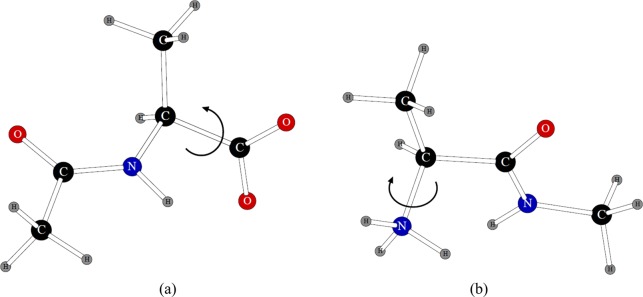
Structures used to fit torsional parameters for the ionized C-terminus (a) and N-terminus (b). Similar systems were used for electrostatically neutral forms of the termini.
The values of the parameters were produced and employed previously.12 Tabulated here are the resulting average errors in the rotamer energies presented in Table 24. It can be seen that all the errors are in the reasonable ca. 0.3 kcal/mol range.
Table 24. Average Deviations (kcal/mol) of POSSIM Energies from Those Obtained by Quantum Mechanical Calculations for the Rotamers Used in Fitting Torsional Parameters for Protein Termini.
| terminus | avg. error in rotamer energies |
|---|---|
| –COO– | 0.18 |
| –COOH | 0.33 |
| –NH3+ | 0.28 |
| –NH2 | 0.32 |
C. Simulations of the Collagen-Like Peptide
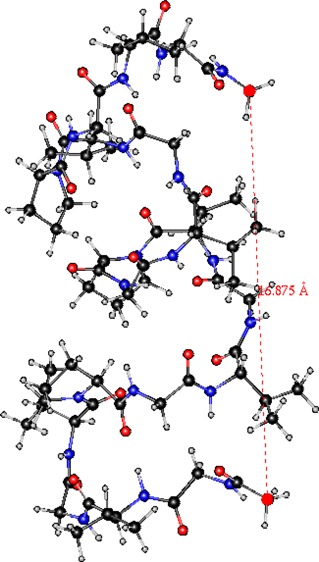
While results of these simulations cannot be considered an exhaustive test of our second-order polarizable POSSIM formalism and parameters, they do provide an illustration of the validity of the technique. The reference 3AH9 geometry and representative structures from the simulations are shown in Figure 7. The RMSD for this snapshot is 0.94 Å, and the maximum deviation is 2.04 Å.
Figure 7.

Structures of the simulated collagen-like peptide: (a) 3AH9 Protein Data Bank geometry; (b) a snapshot from the simulations in this work and (c) the same snapshot with the solvent water molecules and hydrogen atoms removed for clarity.
D. Simulations of the Ac-NGS-NHBn, Ac-QGS-NHBn, and Ac-NPS-NHBn Peptides
Representative structures of these oligopeptides are shown in Figures 8–10.
Figure 8.

Reference structure of the Ac-NGS-NHBn peptide.13
Figure 10.
Reference structure of the Ac-NPS-NHBn peptide.13
Figure 9.

Reference structure of the Ac-QGS-NHBn peptide.13
We have optimized geometries of four previously reported13 conformers for each of the structures. Both the second-order polarizable POSSIM and fixed-charges OPLS-AA force fields were used. The resulting RMSDs are reported in Table 25. The deviations are roughly the same with OPLS-AA and POSSIM for the first peptide. The average error is 1.19 Å with POSSIM and 1.04 Å with OPLS. For the second system, OPLS has an advantage with an average RMSD of 0.51 Å, while the POSSIM result is about 1.01 Å. The level of performance is reversed for the third oligopeptide, as POSSIM performs better with an average RMSD of 0.59 Å, and OPLS yields an average error of 1.02 Å. Overall, it appears that the OPLS-AA and POSSIM performance is approximately the same for these peptides, which is consistent with the dipeptide calculations reported in this article and our previous work on producing polarizable force fields.7,10−12
Table 25. RMSD (in Å) for the Optimized Oligopeptide Structures with Respect to the Reference Geometries13a.
| RMSD |
||
|---|---|---|
| system | POSSIM | OPLS-AA |
| Ac-NGS-NHBn | ||
| conformer 1 | 1.31 | 0.87 |
| conformer 2 | 1.64 | 1.46 |
| conformer 3 | 1.10 | 1.01 |
| conformer 4 | 0.70 | 0.82 |
| avg. RMSD | 1.19 | 1.04 |
| Ac-QGS-NHBn | ||
| conformer 1 | 1.35 | 0.75 |
| conformer 2 | 1.09 | 0.30 |
| conformer 3 | 0.54 | 0.72 |
| conformer 4 | 1.06 | 0.27 |
| avg. RMSD | 1.01 | 0.51 |
| Ac-NPS-NHBn | ||
| conformer 1 | 0.34 | 0.87 |
| conformer 2 | 0.36 | 1.05 |
| conformer 3 | 1.27 | 1.07 |
| conformer 4 | 1.50 | 1.07 |
| avg. RMSD | 0.59 | 1.02 |
Only heavy atoms have been taken into account.
E. Effects of Using the Second-Order Polarization Model
We have been constantly monitoring the results of our second-order polarizable simulations to make sure that the second-order approximation is capable of reproducing physical phenomena as accurately as the full-scale polarization approach. So far, we have seen no indications that it cannot. The main evidence that this formalism works well is that both gas-phase and liquid-state properties can be reproduced with the same set of parameters—something that fixed-charges force fields cannot accomplish consistently because of their lack of explicit many-body effects.
The only case when the second-order polarization model would definitely give qualitatively different results from the full point-dipole model would be for the polarization catastrophe—when the relative position of the dipoles is such that the iterative process for finding the induced dipole values diverges and the dipoles grow without limit. However, this is certainly an undesirable scenario, and full polarization techniques usually employ methods for avoiding this computational artifact anyway.
Let us consider the following illustration. Given in Figure 11 are polarization energies calculated for two particles—one with a charge of +0.5 e, the other with a charge of −0.5 e, and both with polarizabilities of 2.0 Å3—as a function of distance between them. These calculations were performed for the full-scale (eq 3), the second-order (POSSIM, eq 4b), and the first-order (eq 4a) polarizability approaches. It can be seen that significant deviations occur only at short distances, especially if we consider only the full and second-order techniques. At a distance of 2.6 Å, the difference between the two is already ca. 5%, and any deviation at shorter (but still physically relevant) distances can be corrected by proper second-order parametrization. Moreover, the rapid growth in the magnitude of the full-scale polarization energy at short distances is likely to take place in the region where the point-dipole approximation is already less valid. Consider for example, at 1.6 Å the full polarization energy is −1076.32 kcal/mol, much too large to be physically reliable. Therefore, we believe that our second-order model is a robust way to represent many-body interactions that is validated by its ability to reproduce both the gas-phase and liquid-state results.
Figure 11.
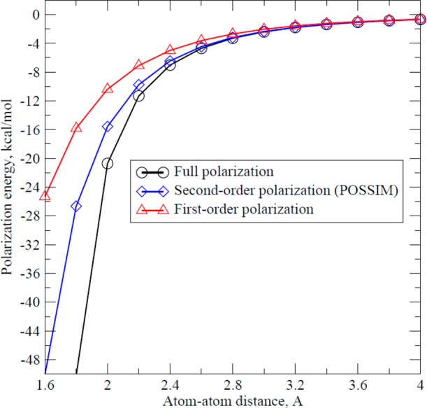
Polarization energy between two particles with charges ±0.5 e and polarizability of 2.0 Å3 as a function of distance between their centers.
It should be emphasized that our second-order POSSIM method does not parametrize the force field for full-scale polarization and then use those parameters in the approximate second-order implementation. All parametrization is done for the second-order polarization approximation, and thus, any systematic differences between the full-scale and second-order approximations are compensated for. Furthermore, even if full-scale polarization were desired, using the second-order POSSIM parameters would likely produce large errors rendering them unusable without significant reparameterization.
We have conducted the following experiment. A pure liquid water configuration was generated. It included 216 POSSIM water molecules. Periodic boundary conditions were imposed. While this was only a single snapshot, it could be used as one of Mone Carlo configurations in simulating a bulk water system. The first-order polarization energy was found to be −742.12 kcal/mol for this system. The second-order POSSIM formalism yielded a polarization energy of −1109.35 kcal/mol. The full-scale converged polarization energy was −1729.75 kcal/mol. Thus, the polarization energy calculated per one water molecule was −3.44, −5.14, and −8.01 kcal/mol with the first-order polarization model, POSSIM, and the complete polarization formalism, respectively. We have already pointed out that our parametrization of the second-order POSSIM model is carried out in such a way as to eliminate possible effects in quantitative differences of magnitudes of polarization energy with the full polarization model. Thus, the above numbers do not indicate any fundamental problem with the POSSIM formalism but rather demonstrate the amount of difference with the full-scale polarization methodology that can be encountered when using the second-order approximation.
In addition to examining the energy results for a pure liquid water snapshot, we have also run full-scale Monte Carlo simulations with the three polarization models. Taking a starting configuration from a previously equilibrated periodic box of 216 POSSIM water molecules and simply changing the order of the polarization calculations from second-order to full-scale and restarting the simulation results in a failure of the simulation after a few thousand MC configurations because of significant growth of the magnitude of polarization energy. Likewise, changing the order of the polarization calculations from second-order to first-order and allowing the system to reach equilibrium lead to the average volume and the magnitude of the average energy being underestimated by about 13% and 30%, respectively. However, the average energy and volume for both simulations can be brought to near agreement with the second-order calculations with minor reparameterization.
Shown in Table 26 are the average total energy, polarization energy, and volume for three polarization models after at least 2 × 10⁶ steps of equilibration followed by at least 5 × 10⁶ steps of averaging for 216 water molecules at 25 °C and 1 atm in a periodic box. Nonbonded cutoffs for dipole–dipole interactions were set to 7 Å and all other nonbonded cutoffs to 8 Å; the usual correction to the Lennard-Jones energy was used. The results for the second-order (POSSIM) model were obtained by adopting the parameters, unchanged, from our previously published water model.10 The full-scale and first-order results were obtained by taking our POSSIM water model and adjusting the oxygen polarizability, while maintaining the ratio of oxygen polarizability to hydrogen polarizability, until the average energy and volume were in best agreement with the second-order averages. Decreasing the second-order polarizabilities by about 21% (from αO/αH = 0.77/0.30 for second-order to αO/αH = 0.61/0.24 for full-scale) brought the full-scale polarizability calculations within 1% and 3% of the average energy and volume respectively of the POSSIM calculations. While increasing the second-order polarizabilities by about 60% (to αO/αH = 1.23/0.49) brought the first-order polarizability calculations within 1% of the average energy and 2% of the average volume of the POSSIM calculations. Interestingly, while the average polarization energy for POSSIM and the first-order calculations is nearly the same (−1128 ± 14 kcal/mol or −5.22 ± 0.06 kcal/mol per molecule for POSSIM and −1100 ± 18 or −5.09 ± 0.08 kcal/mol per molecule for first-order) it is noticeably larger for full-scale polarization (−1411 ± 52 kcal/mol or −6.53 ± 0.24 kcal/mol per molecule). This “extra” polarization energy is balanced by an increase in the stretching and bending energies as well as the slight overestimation of the volume.
Table 26. Average Total Energy, Polarization Energy (Both in kcal/mol), and Volume (in Å3) for POSSIM (Second-Order Polarization), Full-Scale, and First-Order Polarizable Water Modelsa.
| polarization model | total energy | polarization energy | vol. |
|---|---|---|---|
| full-scale | –2001 ± 35 | –1411 ± 52 | 6335 ± 67 |
| 2nd order (POSSIM) | –1987 ± 12 | –1128 ± 14 | 6563 ± 71 |
| 1st order | –2002 ± 19 | –1100 ± 18 | 6665 ± 80 |
The full-scale and first-order models use POSSIM water with refitted polarizabilities. See text for details. Uncertainties given as standard deviations of 2 × 10⁵ configuration averages.
One should keep in mind that there is no guarantee of transferability of these refit water models to other systems. These water models are to demonstrate that a simple reparameterization (only one degree of freedom in parameter space) was able to mostly eliminate the discrepancies between polarization orders of the liquid-phase properties. If a robust first-order or full-scale polarization model of water were desired, we would likely proceed via our standard parametrization methodology (i.e., start by fitting polarizabilites with three-body energies, then fit the partial charges and Lennard-Jones constants using gas-phase dimers, then fine-tune the parameters with liquid simulations).
While the above examples cannot account for all the possible situations, they do serve as an illustration for the statement that the second-order polarization formalism employed in POSSIM is adequate in reproducing many-body effects, provided that a proper parametrization procedure is followed.
IV. Conclusions
We have produced a complete second-order polarizable force field for protein within the POSSIM framework. In validating the values of the parameters, we reproduced dipeptide conformational energies within an average deviation of 0.52 kcal/mol from the quantum mechanical data and achieved an average accuracy of 9.7° for the key dihedral angles. We have performed additional validation by running Monte Carlo simulations of a collagen-like protein in water. The resulting geometries were within 0.94 Å RMSD from the experimental data. Finally, conformational analysis of three oligopeptides related to N-linked glycoproteins has demonstrated that the POSSIM force field performs on par with the OPLS-AA for these systems.
The procedure for fitting the parameters was somewhat simplified compared to that used in building the previous version of the polarized force field for proteins. Even more importantly, we have noticeably reduced the number of parameters used in our formalism. This means two things, First, we have achieved a greater level of transferability by more extensively using small-molecule parameters as those for protein fragments. Second, we reduced the number of parameter types (for example, permanent electrostatic dipoles are no longer employed). In spite of these changes, the average accuracy of the resulting POSSIM force field is at approximately the same level as the previous version of the polarizable force field (PFF) and the all-atom OPLS force field. We are hoping that these changes will further improve the robustness of biophysical simulations involving the polarizable force field.
Moreover, the methodology applied in this work can be applied to other classes of organic and biologically significant molecules. Further validation and application of POSSIM will include extensive simulations of other protein and protein–ligand systems; this has been set as the direction of our current and future work.
Acknowledgments
This project was supported by Grant No. R01GM074624 from the National Institutes of Health. The content is solely the responsibility of the authors and does not necessarily represent the official views of the National Institute of General Medical Sciences or the National Institutes of Health. The authors express gratitude to Schrödinger, LLC, for the Jaguar software.
Supporting Information Available
All the potential energy parameters developed in the course of this work; details on parameter fitting for specific amino acids. This material is available free of charge via the Internet at http://pubs.acs.org.
The authors declare no competing financial interest.
Funding Statement
National Institutes of Health, United States
Supplementary Material
References
- See, for example; a Caldwell J. W.; Kollman P. A. J. Am. Chem. Soc. 1995, 117, 4177–4178. [Google Scholar]; b Jiao D.; Zhang J. J.; Duke R. E.; Li G. H.; Schneiders M. J.; Ren P. Y. J. Comput. Chem. 2009, 30, 1701–1711. [DOI] [PMC free article] [PubMed] [Google Scholar]
- a MacDermaid C. M.; Kaminski G. A. J. Phys. Chem. B 2007, 111, 9036–9044. [DOI] [PubMed] [Google Scholar]; b Click T. H.; Kaminski G. A. J. Phys. Chem. B 2009, 113, 7844–7850. [DOI] [PMC free article] [PubMed] [Google Scholar]
- Veluraja K.; Margulis C. J. J. Biomol. Struct. Dyn. 2005, 23, 101–111. [DOI] [PubMed] [Google Scholar]
- Click T. H.; Ponomarev S. Y.; Kaminski G. A. J. Comput. Chem. 2012, 33, 1142–1151. [DOI] [PMC free article] [PubMed] [Google Scholar]
- Ji C.; Mei Y.; Zhang J. Z. H. Biophys. J. 2008, 95, 1080–1088. [DOI] [PMC free article] [PubMed] [Google Scholar]
- a Jiang W.; Hardy D. J.; Phillips J. C.; MacKerell A. D.; Schulten K.; Roux B. Phys. Chem. Lett. 2011, 2, 87–92. [DOI] [PMC free article] [PubMed] [Google Scholar]; b Vorobyov I.; Bennett W. F. D.; Tieleman D. P.; Allen T. W.; Noskov S. J. Chem. Theory Comput. 2012, 8, 618–628. [DOI] [PubMed] [Google Scholar]; c Baker C. M.; Lopes P. E. M.; Zhu X.; Roux B.; MacKerell A. D. J. Chem. Theory Comput. 2010, 6, 1181–1198. [DOI] [PMC free article] [PubMed] [Google Scholar]; d Ponder J. W.; Wu C.; Ren P.; Pande V. S.; Chodera J. D.; Schneiders M. J.; Haque I.; Mobley D. L.; Lambrecht D. S.; DiStasio R. A.; Head-Gordon M.; Clark G. N. I.; Johnson M. E.; Head-Gordon T. J. Phys. Chem. B 2010, 114, 2549–2564. [DOI] [PMC free article] [PubMed] [Google Scholar]; e Marjolin A.; Gourlaouen C.; Clavaguera C.; Ren P. Y.; Wu J. C.; Gresh N.; Dognon J.-P.; Piquemal J.-P. Theor. Chem. Acc. 2012, 131, 1198–1211. [Google Scholar]; f Case D. A.; Cheatham T. E.; Darden T.; Gohlke H.; Luo R.; Merz K. M.; Onufriev A.; Simmerling C.; Wang B.; Woods R. J. Comput. Chem. 2005, 26, 1668–1688. [DOI] [PMC free article] [PubMed] [Google Scholar]; g Rick S. W.; Stuart S. J.; Berne B. J. J. Chem. Phys. 1994, 101, 6141–6156. [Google Scholar]
- Kaminski G. A.; Stern H. A.; Berne B. J.; Friesner R. A.; Cao Y. X.; Murphy R. B.; Zhou R.; Halgren T. J. Comput. Chem. 2002, 23, 1515–1531. [DOI] [PMC free article] [PubMed] [Google Scholar]
- Kaminski G. A.; Friesner R. A.; Tirado-Rives J.; Jorgensen W. L. J. Phys. Chem. B 2001, 105, 6474–6487. [Google Scholar]
- Kaminski G. A.; Zhou R.; Friesner R. A. J. Comput. Chem. 2003, 24, 267–276. [DOI] [PubMed] [Google Scholar]
- Kaminski G. A.; Ponomarev S. Y.; Liu A. B. J. Chem. Theory Comput. 2009, 5, 2935–2943. [DOI] [PMC free article] [PubMed] [Google Scholar]
- Ponomarev S. Y.; Kaminski G. A. J. Chem. Theory Comput. 2011, 7, 1415–1427. [DOI] [PMC free article] [PubMed] [Google Scholar]
- Ponomarev S. Y.; Sa Q.; Kaminski G. A. J. Chem. Theory Comput. 2012, 8, 4691–4706. [DOI] [PMC free article] [PubMed] [Google Scholar]
- Cocinero E. J.; Stance-Kaposta E. C.; Gamblin D. P.; Davis B. G.; Simons J. P. J. Am. Chem. Soc. 2009, 131, 1282–1287. [DOI] [PubMed] [Google Scholar]
- Li X.; Ponomarev S. Y.; Sa Q.; Sigalovsky D. L.; Kaminski G. A. J. Comput. Chem. 2013, 34, 1241–1250. [DOI] [PMC free article] [PubMed] [Google Scholar]
- a Jaguar v3.5, Schrödinger, Inc.: Portland, OR, 1998.; b Jaguar v4.2, Schrödinger, Inc.: Portland, OR, 2000.; c Jaguar v7.6, Schrödinger, LLC, New York, 2009.
- Kaminski G. A.; Maple J. R.; Murphy R. B.; Braden D.; Friesner R. A. J. Chem. Theory Comput. 2005, 1, 248–254. [DOI] [PubMed] [Google Scholar]
- RCSB Protein Data Bank. http://www.rcsb.org/pdb/home/home.do (accessed June 18, 2014).
- McDonald N. A.; Jorgensen W. L. J. Phys. Chem. B 1998, 102, 8049–8059. [Google Scholar]
Associated Data
This section collects any data citations, data availability statements, or supplementary materials included in this article.