The Difference-in-Difference Method: Assessing the Selection Bias in the Effects of Neighborhood Environment on Health

Abstract

This paper uses the difference-in-difference estimation approach to explore the self-selection bias in estimating the effect of neighborhood economic environment on self-assessed health among older adults. The results indicate that there is evidence of downward bias in the conventional estimates of the effect of neighborhood economic disadvantage on self-reported health, representing a lower bound of the true effect.

Introduction

There has been an explosion of literature in the past 15 years focusing on the effect of neighborhood environment on various health outcomes. This includes studies of self-assessed health (Inagami et al., 2007), chronic conditions, disability (Wight et al., 2008), body weight (Ackerson et al., 2008; Do et al., 2007; Powell and Bao, 2009), and height (Do et al., 2013). With the exception of the Moving to Opportunity Project (MTO), a randomized trial of housing location, this literature has been based on observational studies. In these studies, one or more neighborhood environment characteristics are included in a regression model that controls for individual, family and demographic characteristics. The regression model is typically estimated as a two-level regression model, where individuals at the first level are nested within neighborhoods at the second level.

Naturally, such an approach may suffer from estimation bias due to the non-random nature of the neighborhood selection process by individuals. It is not obvious that self-selection into a neighborhood would actually produce a bias. This would only be the case if individual health is a factor in choosing the type of neighborhood that a person wants to live in. Further, the direction of any existing bias provides important information for informing potential causal inferences. In the case of an upward bias, the estimates generated would be an upper bound on the true effects of neighborhoods on health. On the other hand, if there is a downward bias, then the estimates generated would be a lower bound on the true effects of neighborhoods on health. The papers that use the traditional estimation approach described above typically recognize the potential for selection bias but do not attempt to address it. The problem of the potential self-selection bias has been documented in the literature (Oakes, 2004, 2006) but there have not been to our knowledge any attempts to understand the direction of the bias and its implications for making causal inferences. This paper addresses this issue by using a longitudinal data set, the US Health and Retirement Study.

After using a traditional two-level model (that models individuals nested within neighborhoods) to estimate the relationship between neighborhood environment and health, we use the difference-in-difference estimation technique to assess the direction of the self-selection bias. Specifically, we use the Health and Retirement Study as our main data source and self-assessed health among the elderly as a health outcome of interest. Since it is not possible to create an unbiased estimator, we cannot estimate the size of the bias, but instead assess the direction of the bias, and its implications for making causal inferences. The findings indicate that it is likely that for the particular data, time period, and outcome examined, the traditional approach may produce a downward bias. In other words, for the specific example considered we find indications of underestimating the effect of neighborhood environment on health. Thus, conventional estimates for our example are a lower bound of the true estimate.

Previous Research

Self-selection bias is an important concern in the neighborhoods literature. Moreover, self-selection bias seems to be a potential estimation issue not only in observational studies but in experimental studies as well (Clampet-Lundquist and Massey, 2008). The general agreement is that the direction of self-selection bias that may both be upward or downward (Duncan et al., 1997; Dustmann and Preston, 2001; Leventhal and Brooks-Gunn, 2000). Previous studies tend to make explicit or implicit assumptions regarding the direction of the self-selection bias and then aim to correct the bias under these assumptions. These studies do not tend to analyze the direction of the self-selection bias or the self-selection mechanism that resulted in the bias.

For instance, there is a vast literature that concentrates on the role of neighborhood economic disadvantage factors, such as neighborhood poverty, in shaping population health and well-being disparities. There has been a concern in this literature that self-selection may lead to underestimation of the effects of neighborhood poverty on health. To illustrate, Clampet-Lundquist and Massey (2008) argue that in the Moving to Opportunity experiment selective migration out of new homes may have led to underestimation of neighborhoods effects (Clampet-Lundquist and Massey, 2008). The authors suggest addressing this underestimation bias by accounting for the length of time during which individuals were exposed to a particular neighborhood factor. While there are some concerns that this may not solve the estimation issue and may introduce new forms of selection bias (Sampson, 2008) there are a number of observational studies that follow this idea. These observational studies argue that using short term rather than long term measures of exposure to neighborhood environment leads to underestimation of neighborhoods effects (see e.g. (Do, 2009)). However, assuming that self-selection may result in overestimation of neighborhood effects and then applying various methodological approaches to correct the bias is the most frequent approach in the social science literature.

Several methodological approaches have been used to address this potential for self-selection into and out of neighborhoods. First, some authors (Cao et al., 2006; Eid et al., 2008) introduce a larger set of controls, including individual self-reported preferences for the neighborhood environment (Cao et al., 2006). However, with this approach it may not possible to control for all relevant confounders so that the estimated effect of the neighborhood environment could still be biased. Second, other studies have used panel data methods, such as fixed effects estimation (Do and Finch, 2008) and first differencing (Eid et al., 2008) to account for unobserved confounders. These methods account for any type of time-invariant confounders but not time-variant confounders. As an example of the latter, an individual could experience a sudden health shock that would affect the choice of future neighborhood of residence. Another challenge with implementing these methods is that fixed effects and first differencing require sufficient variation in the neighborhood environment over time to estimate the models. If the panel data time span is relatively short, or neighborhoods have not changed substantially over the time period, or very few individuals moved, there may not be sufficient variation in the neighborhood environment to identify the effect of the neighborhood environment on health. Hence, long term longitudinal data with large panel sizes are needed for such analyses.

Third, some authors use sample selection models (Cao, 2009) to adjust for the self-selection bias. This method classifies neighborhoods into two types and does not allow consideration of multiple neighborhood environment characteristics or neighborhood features that vary continuously. Fourth, propensity score matching has been used to adjust for self-selection (Cao et al., 2010). Since the computation of propensity scores is based on observed characteristics this method does not allow for self-selection bias due to unobserved characteristics

Fifth, some authors recognize the potential bias introduced by nonrandom moves and limit their analyses to subsamples of individuals who change neighborhoods over the study time period (Eid et al., 2008; Plantinga and Bernell, 2007). For example, Plantinga and Bernell (2007) examine the effect of urban sprawl on the individual Body Mass Index (BMI) by estimating a model for the decision to move to high- and low- sprawling counties. They find that BMI is a significant determinant of the decision to move to a dense versus sprawling location, indicating the presence of self-selection bias.

Finally, some authors use natural experiments to address the self-selection bias (Anderson and Matsa, 2011; Courtemanche and Carden, 2011; Currie and Walker, 2011; Dunn, 2010; Zhao and Kaestner, 2010). These studies focus on the health effects of local air pollution or the local food environment or local population density. The authors use the introduction of E-ZPass, a Walmart Supercenter expansion pattern, and interstate system expansion as a source of exogenous variation in local neighborhood conditions and apply various estimation techniques, such as instrumental variables (Anderson and Matsa, 2011; Courtemanche and Carden, 2011; Dunn, 2010; Zhao and Kaestner, 2010) and difference-in-difference models (Currie and Walker, 2011). As reviewed earlier, the most consistent result in the neighborhoods literature concerns a strong association between neighborhood economic environment and various health outcomes. Yet, we are not aware of studies that would address the question of health-based self-selection in the context of neighborhood economic environment based on the natural experiment approach.

Self-Selection Bias

The concern that the non-random nature of residential mobility (Golant, 1987; Litwak and Longino, 1987) may bias the estimated effect of the neighborhood environment on health is evident throughout this entire literature. In order for the non-randomness of residential choice to bias the estimated effect of neighborhood environment on health, individual selection of neighborhood environment must be done with his or her own health in mind (Oakes, 2004, 2006). From the statistical standpoint, self-selection bias is one example of potential omitted variable bias. So, what type of residential decisions should researchers be concentrating on in the context of the self-selection bias? Whether an individual decides to stay in, or move from, the current neighborhood of residence, he or she is making a decision involving, in part, the neighborhood environment. Individuals may selectively prefer to stay in, to move out of, or to move to certain types of neighborhoods. The decision to stay in a neighborhood of residence does not require any action on behalf of individuals but it could be selective nonetheless. In fact, in his critique of the neighborhoods literature Oakes (2004) notes the importance of estimating a selection equation as “focus now is therefore turned toward identifying background factors related to people moving to or residing in their neighborhoods.” In other words, in studying the self-selection bias one should concentrate both on individuals who change their neighborhood environment by moving to another neighborhood and on individuals who stay and experience neighborhood environment change around them.

One of the challenges in examining what may or may not result in the self-selection bias is that there is a very important distinction between health-motivated decisions to relocate and health influencing the choice of neighborhood environment. One does not necessarily imply the other and vice versa. For example, once the health of older adults starts failing they sometimes choose to move closer to their children. After the move, the older adult would live at or near the neighborhood of residence of their child. This implies that the neighborhood environment that the older adult lives in after the move is influenced primarily by the residential decisions of his or her children. In other words, in this case health would influence the decision to move but it is unlikely to influence the choice of neighborhood environment. The neighborhood environment was chosen by an adult child and it may have happened years before the older parent decided to move. Thus, this type of residential move is unlikely to result in self-selection bias.

There are also examples when the residential move is not influenced by health while the choice of neighborhood environment is. For instance, after retirement an older adult may decide to relocate to Florida as many older adults do. However, a choice of a particular neighborhood where he or she is going to reside may be influenced by his or her preference for neighborhood environment features. For instance, the older adult may specifically choose the neighborhood that has high walkability, sidewalks, and easy access to healthy food stores. In this case, the residential move is not influenced by health while the choice of neighborhood environment is. This type of residential move is likely to result in self-selection bias.

This paper concentrates on whether the self-selection bias is present and what direction it may go rather than on analyzing specific residential decision pathways that may result in the selection bias. For the purpose of assessing the potential self-selection bias while it may be important to understand why individuals may decide to move it is much more important to understand how they move and whether the change in neighborhood characteristics they live in is related to their health.

When an individual relocates he or she moves out of one neighborhood into another neighborhood. It is important to recognize that the reasons governing one’s choice of moving out of the neighborhood may not necessarily be the same as the reasons for the choice of a new neighborhood. The demography literature even uses two separate terms when describing residential relocation: “in-migration” and “out-migration”. Using this terminology we can say that both the in-migration decision and out-migration decisions may be the source of self-selection bias in neighborhoods research. Both the decision to stay in a neighborhood and the decision to move out of neighborhood are equally important to study. The decision to stay in/move out of a neighborhood may be a potential source of bias. The non-random nature of the decision to stay in /move out of one’s present neighborhood (“out-migration”) has long been recognized in the social science literature. For instance, the Tiebout hypothesis and “white flight” hypothesis that date to the 1950s suggest that the decision to stay in one’s present neighborhood may be influenced by local public good provision and neighborhood racial composition (Duncan and Duncan, 1957; Tiebout, 1956). The recent empirical evidence continues to support these hypotheses (Banzhaf and Walsh, 2008; Pais et al., 2009). In summary, there is a long standing tradition in social science research that recognizes that not only a decision to move to a particular neighborhood may be non-random but a decision to stay in/move out of the present neighborhood may also be non-random.

Unfortunately, this literature does not focus much on how health influences the choice of neighborhood environment, which is the actual source of self-selection bias in statistical estimation in the neighborhoods and health literature. This implies that while studying the bias one needs to keep in mind that it not the choice to move but a choice of neighborhood environment decisions that one needs to focus on.

Overall, the previous literature has two main limitations. First, it tends to recognize a choice to move as a potential source of selection bias but does not in general recognize a decision to stay in the neighborhood as a potential source of self-selection bias. Second, the existing literature does not tend to distinguish between the questions of why and how individuals move. Both of these are important in assessing the presence of selection bias. This paper recognizes that both the decision to “stay in/move out” (out-migration) and the decision “to move to“ another neighborhood (in-migration) are potential sources of bias. Moreover, the analysis is conducted separately for the samples of movers and stayers exactly because we recognize the decisions of “out mobility” may be a potential source of bias.

Focus on the Difference-in-Difference Methodology

This paper uses a technique common in economic studies, the difference-in-difference method to assess the selection bias due to the potentially non-random choice of neighborhood environment. It focuses on a particular example: the relationship between positive self-assessed health status and neighborhood economic environment among older adults.

There has been consistent evidence that neighborhood environment is associated with a variety of health outcomes among older adults, including self-assessed health, disability, obesity, and chronic conditions (Freedman et al., 2008; Grafova et al., 2008; Wight et al., 2008). One of the strongest results in this particular literature and in the general literature on health effects of neighborhood environment has been a strong association between neighborhood economic environment and health. For example, older adults who live in economically disadvantaged neighborhoods are more likely to report being in worse health¹. Conversely, higher neighborhood economic advantage is positively related to the chances of reporting better health among older adults².

The paper consists of two parts. In the first part, we use the 2000 wave of the Health and Retirement Study to estimate conventional cross-sectional multi-level models that estimate the relationship between neighborhood economic environment and self-assessed health. This analysis concentrates on self-assessed health as an outcome variable, which is the research question of interest in studying the role of neighborhoods in the health of populations. In the second step, we examine whether cross-sectional estimates that are based on the 2000 wave of the HRS are potentially subject to self-selection bias and, if so, what the direction of such a bias would be. This analysis focuses on neighborhood economic environment as outcome variables, which is the methodology that permits assessment of the direction of the potential selection bias when longitudinal data are available.

To assess this self-selection bias implies the need to assess whether and how health status may influence the choice of neighborhood environment among older adults. Since the conventional two-level model used in this paper is based on the 2000 wave of the HRS, one of the critical components of such an analysis is to have data on changes in the neighborhood economic environment prior to the 2000 wave. It follows from the discussion above that both changes in the neighborhood economic environment that are due to residential mobility and that are due to the evolution of neighborhoods themselves should be measured. The HRS allows us to reconstruct changes in the neighborhood economic environment experienced by individuals between 1992 and 2000. Another critical data component provided by the HRS is individual health status in the 1992 wave. To assess the selection bias we need to understand to what extent 1992 health status may have influenced neighborhood environment choice between 1992 and 2000.

Once both essential data components are in place, neighborhood environment history and baseline health status, we can examine whether baseline health status is related to changes in neighborhood economic environment. To do this we apply the difference-in-difference methodology. We concentrate on the change in neighborhood economic environment between the 2000 and 1992 waves of the HRS that reflects how the neighborhood economic environment in the 2000 wave (after the 1992–2000 residential decisions were made) and in 1992 (before the 1992–2000 residential decisions were made) differ from one another. The difference-indifference analysis compares this 1992–2000 change in neighborhood environment by baseline health status. Relating baseline health to changes in neighborhood environment that happened after the baseline time period sheds light not only on the question of whether traditional regression analysis is likely to be subject to a bias but also on the question of what direction this bias may be.

Data

Sample

The Health and Retirement Study (HRS) is a longitudinal, nationally representative survey of non-institutionalized older adults that is conducted by the University of Michigan and funded by the U.S. National Institute on Aging. The survey, which began in 1992 and has been fielded biennially thereafter, collects extensive information on health, demographic, and socioeconomic characteristics of respondents ages 51 and older and their spouses. The panel survey is replenished every 6 years and sample weights are provided that adjust for non-response and loss to follow up, so that the survey maintains its ability to provide nationally representative cross-sectional estimates in each year. We follow the initial cohort of age-eligible respondents (who were born between 1931 and 1941 and initially resided in the community) from the beginning of the survey in 1992 through the 2000 wave. There were 9,813 respondents in the 1992 wave of the HRS who resided in the community at the time of the interview. We applied several restrictions to this sample. We excluded 64 respondents with zero sample weights; 305 respondents who were not 51–61years old at the time of the 1992 interview; 847 respondents who died by the 2000 wave of the HRS; 42 respondents who resided in nursing homes at the time of the 2000 interview; 271 respondents who were not interviewed in the 2000 wave due to attrition; 1148 respondents with a missing geocode link, and 369 respondents with missing data. These exclusions resulted in a final sample consisting of 6,767 respondents which includes 3,683 women and 3,084 men.

Self-Assessed Health

The health outcome measure is self-assessed health, as this measure is available and consistently measured in both the 1992 and 2000 waves of the HRS. The survey in both years asks the question “Would you say your health is excellent, very good, good, fair, or poor?” These categories were collapsed to create a dichotomous outcome of self-assessed health: a score of 1 represents excellent or very good health and 0 represents poor, fair, or good health. Self-assessed health has been used extensively in health research as an alternative for more objective health measures and has been shown to be related to mortality, chronic conditions, disability and other health outcomes (Goldstein et al., 1984; Idler and Benyamini, 1997).

The outcome measure used reflects a positive rating of health rather than a negative rating of health, such as poor self-assessed health. The principal difference between positive and negative ratings of health is in how the individuals who reported being in “good” health are treated. If one concentrates on negative health ratings one tends to group individuals in good health with individuals in excellent or very good health. If one concentrates on a positive health rating one tends to focus on individuals in excellent and very good health, grouping individuals in good health together with individuals in poor and fair health. The distinction between these two classification systems is non-trivial: about 28% of men and 27% of women report being in “good” health in 1992. About 29% of men and 30% of women are classified as being in very good health in the 1992 wave. Also, 25% of men and 22% of women are classified as being in excellent health in the 1992 wave. Men and women in fair health constitute 12% and 14% of the sample respectively. Finally, 6% of men and 7% of women are in poor health. Positive and negative ratings of one’s health are not simple opposites. They tend to be determined by different factors (Shooshtari et al., 2007) and reflect different concepts. A positive rating of health more accurately reflects some recent trends among older adults. After active career and parenting ends, and before the onset of illness and terminal decline begins, many older adults enjoy a period of time that brings them ample opportunities for personal fulfillment. This stage of life is often referred to as the third age (James and Wink, 2006). The third age is a fairly recent phenomenon that is a result of increasing lifespans (Sorensen, 2006). During this period of time, people tend to maintain a moderately favorable impression of their own health (McCullough and Polak, 2006). In order to better reflect this recent phenomenon, we concentrate on positive ratings of health rather than on negative ratings of health. The construct of excellent/very good health versus good/fair/poor has been used in the validation of measures of successful aging (Young et al., 2009).

Neighborhood Advantage and Disadvantage Scales

Neighborhoods of residence are defined as areas of about 4,000 people according to the official 1990 Census tract boundaries determined by the U.S. Bureau of the Census. Although tract boundaries do not necessarily match neighborhood boundaries, they are a reasonable approximation of neighborhoods, especially since census tract boundaries “are intended to contain populations reasonably homogeneous with regard to socioeconomic composition” (Kreiger et al., 2003). Using the 1990 Census boundaries in both 1992 and 2000 (rather than relying on 1990 boundaries for 1992 and 2000 boundaries for 2000) is critical because a large proportion (49%) of tracts changed boundaries over this time period (Tatian, 2003). If a person’s census tract of residence is different in 2000 from that of 1992 he or she is classified as being a mover. If a person resides in the same census tract in both 1992 and 2000 then a person is classified as being a stayer. Thus, individuals who may have moved within a census tract are not classified as movers³. The final analytic sample used in the project consists of 6,767 respondents residing in 1,327 census tracts. The sample includes 3,683 women residing in 1,193 census tracts and 3,084 men residing in 1,110 census tracts.

RAND’s Center for Population Health and Health Disparities (CPHHD) created neighborhood measures for both 1990 and 2000 in terms of 1990 Census tract boundaries. Thus, we were able to link the 1990 neighborhood environment measures (for 1990 Census tract boundaries) to the 1992 wave of the HRS and the 2000 neighborhood environment measures (also for 1990 Census tract boundaries) to the 2000 wave of the HRS. Measures were drawn primarily from the 1990 and 2000 Census and also from the Environmental Protection Agency’s Air Quality System.

Because many neighborhood measures are highly correlated, we followed previous studies (Freedman et al., 2008; Grafova et al., 2008) and formed scales for each year by applying confirmatory factor analysis to neighborhood environment characteristics. Items that loaded together at .40 or higher were standardized and added together.

Two scales reflecting the economic circumstances of the neighborhood were formed for each year: one reflecting economic disadvantage and the other economic advantage. Economic disadvantage is characterized by Census tract measures of the percentage of the total population in poverty, the percentage of the population 65 years and older in poverty, the percentage of households receiving public assistance income, the unemployment rate among persons aged 16 years and older, the percentage of housing units without a vehicle, and the percentage of the population that is black. Economic advantage is characterized by the upper quartile value of owner-occupied housing units in the tract; the percentage of families with total annual income of $75,000 (in 1990 dollars) or more; and the percentage of adults with a college degree.

We formed three additional scales reflecting additional neighborhood features that are likely to be correlated with both individual self-assessed health and the economic conditions of the neighborhood: immigration concentration, residential stability, and air pollution. Immigration concentration is measured by: the percent of the population that is Hispanic, the percent of the population that is foreign born, the percent of the population with limited English skills, and a county-level Hispanic isolation index. Residential stability is characterized by: the percentage of the population that lived in the same house for the past 5 years and the median number of years of residence in the housing unit. Finally, air pollution is measured by: four quarterly measures of Particulate Matter at 10 micrometers or less (PM10) and a summertime ozone average.

Cronbach’s alpha’s for these scales fell in the range of 0.85 to 0.92 for 1990 and 0.89 to 0.92 for 2000, indicating a high degree of internal consistency. Each scale has been standardized for ease of interpretation and comparison across scales; thus, a one-unit change in a given scale represents a change of one standard deviation. Consistent with the insight from the Heymann and Fischer model (Heymann and Fischer, 2003) the scales were moderately correlated with the highest correlation as expected between the economic disadvantage and economic advantage scales (the person-level correlation is −0.46 in 1990 and −0.44 in 2000).

Individual-Level Predictors

In the regression models we also included individual-level predictors that are likely to be related to both self-assessed health and the economic attributes of one’s neighborhood of residence. Specifically we included age, race, ethnicity, education, marital status, total household assets, the income-to-needs ratio based on the husband and wife’s earnings, current census region of residence, whether the interview was provided by a proxy respondent, current and previous smoking status and region of birth. The economic data in the HRS are of particularly high quality, with very low rates of missing information on income and assets (Hurd et al., 2003). Frequency distributions for 1992 and 2000 are shown in Table 1.

Table 1.

Sample Characteristics, 1992 and 2000 (Weighted % or Mean)

	1992		2000
	Men	Women	Men	Women
Age, years	55.6	55.7	63.3	63.4
Race/ethnicity
White - omitted category	84.1	82.2	84.1	82.2
Black	8.1	10.4	8.1	10.4
Other	2.2	2.1	2.2	2.1
Hispanic	5.6	5.3	5.6	5.3
Proxy response	6.7	1.5	12.0	2.9
Completed education (years)
≤ 8	10.0	7.8	10.0	7.8
9 – 11	12.6	15.8	12.6	15.8
12	32.4	40.8	32.4	40.8
13 + - omitted category	45.0	35.6	45.0	35.6
Marital status
Married – omitted category	84.6	72.7	82.5	64.3
Widowed	1.6	9.0	3.6	17.9
Divorced/separated	10.2	15.0	10.3	14.5
Never married	3.7	3.3	3.6	3.3
Assets (in $100,000)	2.7	2.4	4.9	4.0
Income category
Poor (<100% poverty line)	6.0	10.5	6.0	10.8
Near poor (<130% poverty line)	2.1	3.0	3.4	4.3
Working class (130% - <185% poverty line)	4.7	6.2	5.7	9.8
Moderate income (185% -<300% poverty line)	10.8	15.7	14.1	18.3
High income (300% or higher poverty line) – omitted category	76.3	64.6	70.6	56.9
Smoking status
Current	24.9	24.5	18.2	16.9
Former	72.2	54.4	72.5	54.6
Current region
Northeast – omitted category	21.4	22.8	20.1	21.3
South	33.2	31.3	35.1	33.4
Midwest	24.6	26.0	24.2	25.1
West	20.8	19.9	20.6	20.1
Region of birth
Northeast – omitted category	22.6	21.5	22.6	21.5
South	30.8	31.9	30.8	31.9
Midwest	28.7	27.9	28.7	27.9
West	9.4	9.5	9.4	9.5
Foreign born	8.5	9.1	8.5	9.1
Number of observations	3,084	3,683	3,084	3,683

Methods

We first examine the relationship between self-assessed health and neighborhood economic advantage and neighborhood economic disadvantage by estimating cross-sectional two-level random-intercept logistic regression models for the year 2000:

$$VGE\_{\mathit{2000}}_{ij}={\alpha }_{\mathit{0}}+{\beta }_{\mathit{0}}NBE\_{\mathit{2000}}_j+{\beta }_{\mathit{1}}NEIGH\_{\mathit{2000}}_j+{\gamma }_{\mathit{0}}X\_{\mathit{2000}}_{ij}+{\epsilon }_{\mathit{0}ij},$$ (1)

VGE_2000_ij is a dummy variable that equals 1 if a respondent i residing in the neighborhood j reports being in excellent or very good health in the 2000 wave. NBE_2000_j includes neighborhood economic advantage and neighborhood economic disadvantage. Following the Heymann and Fischer (2003) model of how neighborhood environment affects aging we included into the vector of variables X_2000_ij individual and family factors, such as age, education, marital status, income, assets, etc. NEIGH_2000_j includes neighborhood immigration concentration, neighborhood residential stability and neighborhood air pollution scales. Standard errors were adjusted to take into account geographic clustering at the Census tract level. The models are stratified by gender for consistency with the neighborhoods literature (Stafford et al., 2005). We then explored the potential for selection bias due to residential selection using both descriptive and multivariate analyses

Changes in Neighborhood Economic Environment over Time

Neighborhood environment changes over time for all individuals, whether individuals move or do not move. Those who move are likely to experience a particularly large change in the neighborhood environment at the time of the move (Quillian, 2003). Those who stay are likely to experience gradual changes in their neighborhood environment over time.

As noted above, to examine whether cross-sectional estimates are potentially subject to self-selection bias, we compare the neighborhood environment change for individuals in better health and individuals in poorer health. There are two distinct groups of people in the sample: movers and stayers. They make very different types of residential decisions. Movers are also likely to face a more abrupt change in the neighborhood environment than stayers. Due to these differences we analyze separately changes over time in the neighborhood environment experienced by these two groups.

To examine the patterns of changes in neighborhood economic environment over time we calculate the differences/changes in neighborhood economic disadvantage and neighborhood economic advantage scales between 1992 and 2000 by baseline health status for both movers and stayers.

Using a series of t-tests we compare the directions in which neighborhoods tend to change for those with different health status. This provides some insights into the potential for residential selection bias. We concentrate on whether the differences in neighborhood features over time differ by health status. To conduct these difference-in-difference tests we use OLS regressions:

$$NB{E}_{it}={\alpha }_{\mathit{1}}+{\beta }_{\mathit{1}}Year{\mathit{2000}}_t+{\gamma }_{\mathit{1}}VGE\_{\mathit{1992}}_i+{\delta }_{\mathit{1}}Year{{\mathit{2000}}_t}^{*}VGE\_{\mathit{1992}}_i+{\tau }_{\mathit{1}}{X}_{it}+{\epsilon }_{\mathit{1}it},$$ (2)

The characteristic NBE_it (either neighborhood economic advantage or neighborhood economic disadvantage) is regressed on the intercept, a time dummy variable Year2000_t that equals 1 for the 2000 wave and 0 for the 1992 wave; a dummy variable VGE_1992_i that equals 1 for individuals who were in excellent or very good health in the 1992 wave and 0 for individuals who were in poor, fair, or good health in the 1992 wave and the dummy variable that is the interaction between these two dummy variables (Year2000_t*VGE_1992_i). To correct for possible confounding, this regression was augmented by all individual-level variables that were used in the two-level random intercept logistic regression models that examined the relationship between the neighborhood environment and self-assessed health.

In order to account for possible gender differences in the effects of neighborhoods on health, these regressions were stratified by gender. The literature on the effects of neighborhood environment on health consistently shows that neighborhood environment may have a different effect on women’s health than on men’s health for a variety of health outcomes, including self-assessed health (Stafford et al., 2005), obesity (Robert and Reither, 2004) and hypertension (Matheson et al., 2009). As noted above, we performed analyses separately for movers and non-movers. Models were stratified by move status between 1992 and 2000⁴. This results in eight difference-in-difference models (2 neighborhood environment characteristics by 2 genders and by 2 types of mobility status).

The interpretation of coefficients in model (2) is not straightforward. For the purpose of the present analysis the coefficient on the year dummy β₁ and the coefficient on the interaction term δ₁ are the most important. It follows from model (2) that the change over time in neighborhood conditions for individuals in very good or excellent health equals the sum of the coefficient on the year dummy and the coefficient on the interaction term:

• (average NBE in the 2000 wave for VGE – average NBE in the 1992 wave for VGE)= (β₁+δ₁).

Similarly, the change over time in neighborhood conditions for individuals in good, fair or poor health equals the coefficient on the year dummy:

• (average NBE in the 2000 wave for nonVGE – average NBE in the 1992 wave for nonVGE) = β₁.

Hence, the interaction term indicates how the change in neighborhood economic disadvantage (or advantage) over time differs by baseline health status:

• [(average NBE in the 2000 wave for VGE – average NBE in the 1992 wave for VGE)-- (average NBE in the 2000 wave for nonVGE – average NBE in the 1992 wave for nonVGE)]=δ₁

Thus, the exact interpretation of the difference-in-difference regression results depends mainly upon the sign and the size of coefficients β₁ and δ₁. Using the estimated sign, size, and statistical significance of the estimated coefficients β₁ and δ₁, the results section discusses the interpretation of the difference-in-difference results in terms of its implications for self-selection bias.

Results

As shown in Table 2, for both men and women, living in more economically disadvantaged areas in 2000 is associated with a lower odds of reporting excellent or very good health whereas living in more advantaged areas is associated with greater odds of reporting excellent or very good health. For men, the former is statistically significant (OR=0.84, 95% CI=0.72, 0.99) whereas the latter is not. For women, the latter is statistically significant (OR=1.11, 95% CI=1.01, 1.21) whereas the former is not.

Table 2.

Neighborhood Effects on Reporting Excellent or Very Good Health: Odds Ratios from Two-level Random Intercept Logistic Regression Models, HRS 2000

	Men (n=3084)	Women (n=3683)
Neighborhood Economic
Characteristics
Disadvantage	0.84 (0.72, 0.99)*	0.92(0.80 1.05)
Advantage	1.08 (0.98, 1.19)	1.11(1.01 1.21)*
Other Neighborhood
Characteristics
Immigration	0.97(0.86 1.09)	0.93(0.83 1.04)
Residential stability	0.95 (0.86 1.05)	0.97(0.89 1.06)
Air pollution	0.98 (0.90 1.07)	0.95(0.88 1.02)
Individual Characteristics
Individual controls in the models included age, race, ethnicity, education, marital status, total household assets, the income-to-needs ratio based on the husband and wife’s earnings, current census region of residence, whether the interview was provided by a proxy respondent, current and previous smoking status and region of birth

^*p<0.05 95% confidence interval shown parenthetically

Each model includes all neighborhood scales and all individual level variables in Table 1.

Residential changes were common over the 8-year period from 1992 through 2000. About 41% of men and 39% of women resided in different tract boundaries in 1992 and 2000⁵. The probability of moving did not differ significantly by initial health status. Among those initially in poor, fair, or good health 40.9% of men and 38.9% of women moved between 1992 and 2000; among those initially in excellent or very good health the figures were 43.1% of men and 40.3% of women, respectively. It seems that health status is not a primary motivation for relocation decisions. This is consistent with our finding that in 2000 only 6–9% of recent movers reported health as being one of the reasons for their last residential move⁶.

Further calculations show that for both men and women there were no significant differences in 1992 in the percentage reporting excellent or very good health status between those who moved and those who did not by 2000. That is, movers and stayers were equally likely to be in excellent or very good health in 1992.

Changes in Neighborhood Economic Environment over Time

Table 3 depicts mean neighborhood economic advantage and disadvantage scores by residential mobility status and gender for the 1992 and 2000 waves of HRS. It is important to remember the difference in the components that comprise economic advantage and disadvantage scales when interpreting the results presented in Table 3. The neighborhood economic disadvantage scale is comprised of items, such as unemployment and poverty rate, that tend to have greater value under worse economic conditions. The neighborhood economic advantage scale is comprised of items, such as by the upper quartile value of owner-occupied housing units that tend to have greater value under better economic conditions.

Table 3.

Mean Neighborhood Score by Residential Mobility Status and Gender: 1992 and 2000

	Stayers		Movers
Neighborhood scale/health status in 1992:	1992/93	2000	1992/93	2000
		Men
Economic disadvantage
Excellent/very good health	−0.32	−0.45**	−0.33	−0.45++
Poor/fair/good health	0.02	−0.19**	−0.04	−0.22++
Economic advantage
Excellent/very good health	0.23	0.40**	0.46*	0.56
Poor/fair/good health	−0.16	0.00**	−0.03	0.06+
N	1,815		1,269
		Women
Economic disadvantage
Excellent/very good health	−0.30	−0.43**	−0.31	−0.44++
Poor/fair/good health	0.18	−0.03**	0.09	−0.14++@
Economic advantage
Excellent/very good health	0.21	0.39**	0.29	0.41
Poor/fair/good health	−0.25	−0.10**	−0.12*	0.00++
N	2,238		1,445

^*p<0.05, ** p<0.01 significantly different from stayers in 1992

+ p<0.05, ++ p<0.01 significantly different from movers in 1992

@ p<0.05 significantly different from stayers in 2000

^**Among stayers, 2000 significantly different from 1992 at p <0.01

⁺Among movers, 2000 significantly different from 1992 at p <0.05

⁺⁺Among movers, 2000 significantly different from 1992 at p <0.01

^#In 1992, movers significantly different from stayers at p <0.05

^@In 2000, movers significantly different from stayers at p <0.05

This creates a difference in interpretation of changes in the economic advantage and economic disadvantage scales. A decline in the economic disadvantage scale signifies improvement in economic conditions. In contrast, for the economic advantage scale, an improvement of economic conditions is associated with an increase in the economic advantage scale.

Table 3 suggests that for most subgroups, neighborhoods improved significantly. Focusing on the top left panel estimates for men, for example, among stayers, neighborhood disadvantage score declined (meaning they showed signs of improvement) and advantage scores increased, for both stayers initially in poor health and those initially in excellent/very good health (significance indicated with *). For example, for male stayers in better health the economic disadvantage score declined from −0.32 in 1992 to −0.45 in 2000 implying an improvement in economic conditions. Similarly, for male stayers in better health the economic advantage score increased from 0.23 in 1992 to 0.40 in 2000 also implying an improvement in economic conditions. The same pattern is seen for women (left side, bottom panel). Among both male and female movers, economic disadvantage improved (the scale declined) irrespective of health status, but economic advantage improved only for those in poor health. Thus, the direction of neighborhood environment change was the same for various groups of older adults: neighborhood economic environment on average improved over time.

In comparing economic disadvantage in 1992 to 2000, Table 3 also demonstrates that male movers and stayers tended to live in similar neighborhoods in terms of economic disadvantage over that time period. However, for women the picture is a bit different. Women movers and stayers tended to live in similar neighborhoods in terms of economic disadvantage in the 1992 wave. However, by 2000, women in poorer health who moved lived in better neighborhoods (with less economic disadvantage) than those who did not move. By 2000, among women in better health those who moved lived in neighborhoods that were similar (in terms of economic disadvantage) to those where women who did not move lived. This may suggest even though neighborhood environment on average improved for various groups of older adults, the improvement was not uniform for all groups

Table 4 depicts estimation coefficients for difference-in-difference regressions that examine the question of whether changes in neighborhood economic environment over time differ by health status⁷. Table 5 summarizes the interpretation of these results.

Table 4.

The Difference-in-Difference Model Estimation Results

	MOVERS		STAYERS
	Female	Male	Female	Male
Neighborhood Economic Disadvantage Wave indicator	−0.26**	−0.26**	−0.25**	−0.26**
(1 for the 2000 wave and 0 for 1992 wave)	(0.05)	(0.05)	(0.04)	(0.03)
Dummy variable for self-assessed health status	−0.17** (0.04)	−0.07 (0.05)	−0.12 ** (0.03)	−0.13** (0.03)
(1 for excellent or very good health in 1992 wave and 0 for good, fair, or poor health in 1992)
Wave indicator * Dummy variable for self- assessed health status	0.14** (0.03)	0.06 (0.04)	0.09** (0.02)	0.08 ** (0.02)
Number of person-year observations	2,890	2,538	4,476	3,630
Neighborhood Economic Advantage Wave indicator	0.19**	0.16	0.12*	0.23
(1 for the 2000 wave and 0 for 1992 wave)	(0.07)	(0.10)	(0.05)	(0.07)
Dummy variable for self-assessed health status	0.14* (0.07)	0.19** (0.08)	0.17** (0.04)	0.13 (0.05)
(1 for excellent or very good health in 1992 wave and 0 for good, fair, or poor health in 1992)
Wave indicator * Dummy variable for self- assessed health status	−0.05 (0.06)	−0.01 (0.07)	0.002 (0.02)	−0.02 (0.02)
Number of person-year observations	2,890	2,538	4,476	3,630

Notes:

^*Significant at 5% level;

^**Significant at 1% level;

Individual controls in the models included age, race (white – reference category, black, other race), ethnicity(non-Hispanic – reference category), education( less than 9 years; 9–11 years; 12 years; more than 12 years – reference category), marital status (married – reference category; widowed, divorced or separated; never married), total household assets and total household assets squared, the income-to-needs ratio based on the husband and wife’s earnings (less than 100% poverty line; less than 130% poverty line; 130–185% poverty line; 185–300% poverty line; more than 300% poverty line – reference category), current census region of residence (South; Midwest; West; Northeast – reference category;), whether the interview was provided by a proxy respondent, current and previous smoking status and region of birth residence (South; Midwest; West; Northeast – reference category; foreign born).

Table 5.

Residential Mobility and Self-assessed Health: Summary of the Difference-in-Difference Analyses

	Men	Women	Interpretation
Changes in Neighborhood Economic Environment over Time
Improvement in terms of neighborhood economic disadvantage is the same/smaller/greater in size for those in poor, fair or good health than for those in excellent or very good health	Greater Among stayers and same among movers	Greater	Those in poor, fair or good health are “catching up”. Indicates potential downward bias.
Improvement in terms of the neighborhood economic advantage is the same/smaller/greater in size for those in poor, fair or good health than for those in excellent or very good health	Same	Same	Difference between those in poor, fair or good health and those in excellent or very good health remains the same. Indicates no bias due to residential mobility.

Table 5 contains interpretation of the difference-in-difference estimation results presented in Table 4 above.

Recall that the sum of the coefficient on the year dummy and the coefficient on the interaction term equals the change over time in neighborhood conditions for individuals in better health and the coefficient on the year dummy equals the change over time in neighborhood conditions for individuals in poorer health. The interaction coefficient equals the difference in the change in neighborhood economic disadvantage (or advantage) over time between individuals in better and poorer health. For instance, consider female stayers. It follows from the third column in Table 4 that the average change in economic disadvantage for female stayer in poorer health equals −0.25. The average change in economic disadvantage for female stayers in better health equals −0.25+0.09=−0.16. The positive interaction term 0.09 shifts the value of a change in economic disadvantage from −0.25 for less healthy women to −0.16 for more healthy women. As Figure 1 depicts this shift toward zero indicates that economic conditions improved to a smaller degree for more healthy women.

Figure 1.

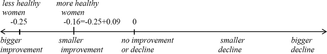
Change in Neighborhood Economic Disadvantage Scale and Improvement or Decline of Economic Conditions

Using a similar exercise we find that among male stayers and women regardless of move status, improvement of economic conditions, as reflected by the neighborhood economic disadvantage is greater for those in poor, fair or good health than for those in excellent or very good health. Given that individuals in poorer health tend to live in more disadvantaged neighborhoods than individuals in better health, this result implies that individuals in poorer health are “catching up” relative to individuals in better health. This difference in neighborhood quality over time by health status is consistent with the presence of residential selection. Further, the observed direction of this selection is such that it may potentially bias the estimated effect of neighborhood economic disadvantage towards the null.

Table 4 also indicates that for the neighborhood economic advantage regression the estimated coefficients on the interaction term are small and insignificant. This indicates that we were unable to find a significant presence of neighborhood economic advantage self-selection. In other words, we do not find evidence suggesting that individuals take their health status into account when choosing the level of neighborhood economic advantage they will to be exposed to.

Taken together, our results seem to suggest that the coefficients on neighborhood economic advantage are likely to be more reliable than the coefficients on neighborhood economic disadvantage since the latter set of coefficients is likely to be underestimated. This is consistent with the previous literature that argues that neighborhood economic advantage is more than just absence of neighborhood economic disadvantage (Massey, 1996; Sampson and Morenoff, 2004). Our results provide further evidence that characterizing neighborhood economic environment only in terms of economic disadvantage and poverty oversimplifies the role of neighborhood economic status on health.

Self-Selection Results and the Grossman Model

As discussed above we find that there is a greater improvement in economic conditions, as reflected by the neighborhood economic disadvantage scale, for individuals in poor, fair or good health than for individuals in excellent or very good health. One explanation for this result is that individuals in poor, fair or good health may choose to live in a neighborhood with better economic environment in order to improve their health.

Specifically, consider older adults who experience a decline in health. It is possible that older adults who experience a decline in health may choose to change their lifestyle in order to invest in their health. This is consistent the Grossman model of the demand for health. According to the Grossman model, a decrease in health causes a loss in utility. The individual stock of health can be replenished by investment into health which may involve a change in lifestyle. The Grossman model predicts that individuals would change their lifestyle if utility loss caused by a decrease in health exceeds the utility loss caused by a change in lifestyle to a healthier one. Older adults who decide to change their lifestyle to a healthier one would face various time and money opportunity costs. These time and money opportunity costs of making such lifestyle changes is likely to be smaller for older adults living in neighborhoods with better economic environment than for older adults living in neighborhoods with worse economic environments. Thus, older adults who want to invest into their health may select to live in neighborhoods with better economic environment because the opportunity costs of the lifestyle changes are smaller is such neighborhoods. From the estimation standpoint, such residential decisions made by older adults with declining health with an aim of improving their health would likely result in the underestimation bias of the effect of economic environment on health.

Discussion

This paper focuses on self-selection bias in the literature that examines the effect of neighborhood environment on health. Two methodological approaches are generally used in the economics literature to deal with estimation biases. The first approach focuses on methods that would yield the exact identification of the treatment effect. The second approach focuses on yielding informative bounds on the treatment effect. Our paper follows the second approach⁸. It suggests that a conventional difference-in-difference approach can be applied to assess the direction of self-selection bias in research on the effects of neighborhoods on health. The paper focuses on a particular example that analyzes how neighborhood economic environment may impact the self-assessed health of older adults. We found evidence that cross-sectional estimates of the effect of neighborhood economic environment on health are underestimated.

One of the important aspects in studying the self-selection bias in the context of neighborhoods and health research is to understand that neighborhood economic features change for both persons who moved and those who do not. Decisions about where to live could bias the cross-sectional estimates if individual health was a factor in the decision-making process of what neighborhood environment an individual wants to live in. By examining how neighborhoods change over time and how the difference in neighborhood quality differs for different groups of people, we examine indirectly whether residential mobility decisions would bias cross-sectional estimates. We found evidence indicating that men and women in poorer health, who tend to live in more disadvantaged neighborhoods, experienced a greater improvement in terms of neighborhood economic disadvantage (disadvantage decreasing) than men and women in better health. For instance, as discussed in the Results section, the average change in the economic disadvantage scale over the 1992–2000 time period equals −0.25 for female stayers in poorer health and −0.16 for female stayers in better health. The negative value of the change in the neighborhood disadvantage scale signifies improvement in terms of neighborhood economic disadvantage. Since abs(−0.25)>abs(−0.16) the absolute value of the improvement in terms of neighborhood economic disadvantage is greater for female stayers in poorer health than for female stayers in better health.

This indicates not only that health is likely to influence the residential decisions of older adults, but also that this selective decision process is likely to result in a downward bias. In other words, cross-sectional estimates of the effect of neighborhood economic environment on health are likely to be underestimated. Thus, we did not find evidence that the observed relationship between neighborhood economic conditions and self-assessed health are due to the selection of better neighborhoods of residence by persons in better health. We did find evidence of residential selection, but it was of such a nature that the effects of neighborhood economic environment on self-assessed health are underestimated, suggesting that the effects estimated here are a lower bound.

Several limitations of this study are noteworthy. This is an observational study and we are unable to prove definitively the presence or absence of self-selection bias. However, examining and comparing the patterns of neighborhood environment change for various groups of people can provide indirect evidence to shed light on this question. Although the difference-in-difference methodology may be useful for exploring bias related to residential mobility or lack thereof, one cannot generalize findings regarding the direction of bias to other neighborhood factors, other health outcomes, or other age groups. Also, the time period studied (1992–2000) was a time of relative economic stability and growth and the results of the study may not necessarily be applicable to different time periods. In addition, the difference-in-difference methodology relies on the assumption of the same trends in the absence of treatment (Meyer, 1995). In the context of our paper we implicitly assume the 1992–2000 change in neighborhood economic environment between individuals in better health and individual in poorer health is caused by differences in their health status.

This study also does not address other potential estimation biases that could originate from selective mortality, selective attrition, or selective mobility into nursing homes. Instead, we address a particular case of an omitted variable bias that could arise from the residential self-selection process. As a sensitivity analysis, we added individuals who died, dropped out of the survey, or moved into a nursing home between the 1992 and the 2000 waves into the regression analysis. To do this, we used their individual and neighborhood characteristics as of the 1992 wave. The results did not change substantially.

In addition, our use of scales limits interpretability to a degree. That is, it is not possible to pinpoint which aspect of economic disadvantage likely influences self-assessed health. In order to explore whether any particular component of the neighborhood economic advantage scale was more relevant, we split the scale into the three components. Then, we re-estimated the model presented in Table 2 by substituting the neighborhood economic advantage scale with each of its three components. We found that the relationship between all three components and health status is very similar and that the relationship between the neighborhood economic advantage scale and health status is not driven by any specific component of the scale. We repeated this sensitivity check for the neighborhood economic disadvantage scale and found a similar result. This finding raises a cautionary note for researchers that multiple features of the neighborhood that are highly correlated may be impossible to disentangle.

Self-selection is not the only possible source of omitted variable bias. It is also possible that some unobserved neighborhood characteristics could be related to both individual health and observed neighborhood characteristics. For instance, individuals with higher valuation for the future are more likely to invest into their health and lead healthier lifestyle than individuals with lower valuation for the future. To accommodate the preferences for healthier lifestyle individuals with higher valuation for the future may be more likely to choose a neighborhood environment that promotes such a lifestyle. Thus, preferences may cause health outcomes and neighborhood environment to be correlated. Examining the role of preferences in neighborhoods and health research is an under-researched area. It is a very important area but it is broad area that goes beyond the scope of this paper.

Despite these limitations, our findings that cross-sectional estimates of the effect of the economic disadvantage on self-assessed health in later life are likely to be downward biased are noteworthy. The literature has focused mainly on potential spurious effects that might stem from people in poor health choosing to live in economically disadvantaged neighborhoods. Our results suggest that bias toward the null may be occurring in part because movers in poorer health may select to move into better neighborhoods in terms of lower neighborhood economic disadvantage than those that they move from and because poor neighborhoods - at least during the 1990s -appeared to improve more than neighborhoods with lower poverty and less economic disadvantage.

• We discuss self-selection bias in neighborhoods and health research literature

• We use difference-in-difference estimation technique examine the self selection bias

• Conventional estimates underestimate the effect of economic environment on health

References

- Ackerson LK, Kawachi I, M BE, Subramanian SV. Geography of underweight and overweight among women in India: A multilevel analysis of 3204 neighborhoods in 26 states Economics & Human Biology. 2008;6:264–280. doi: 10.1016/j.ehb.2008.05.002. [DOI] [PMC free article] [PubMed] [Google Scholar]
- Altonji JG, TE E, R TC. Selection on observed and unobserved variables: Assessing the effectiveness of Catholic schools. Journal of Political Economy. 2005;113:151–184. [Google Scholar]
- Anderson M, Matsa D. Are restaurants really supersizing America? American Economic Journal: Applied Economics. 2011;3:152–188. [Google Scholar]
- Banzhaf HS, Walsh RP. Do people vote with their feet? An empirical test of Tiebout's mechanism. American Economic Review. 2008;93:843–863. [Google Scholar]
- Brown AF, Ang A, Pebley AR. The relationship between neighborhood characteristics and self-rated health for adults with chronic conditions. American Journal of Public Health. 2007;97:926–932. doi: 10.2105/AJPH.2005.069443. [DOI] [PMC free article] [PubMed] [Google Scholar]
- Cagney KA, Browning CR, Wen M. Racial disparities in self-rated health at older ages: what difference does the neighborhood make? Journals of Gerontology Series B: Psychological Sciences and Social Sciences. 2005;60:S181–S190. doi: 10.1093/geronb/60.4.s181. [DOI] [PubMed] [Google Scholar]
- Cao XY. Disentangling the influence of neighborhood type and self-selection: an application of sample selection method. Transportation. 2009;36:207–222. [Google Scholar]
- Cao XY, Handy SL, Mokhtarian PL. The influences of the built environment and residential self-selection on pedestrian behavior: Evidence from Austin, TX. Transportation. 2006;33:1–20. [Google Scholar]
- Cao XY, Xu Z, Fan Y. Exploring the connections among residential location, self-selection, and driving: Propensity score matching with multiple treatments. Transportation Research Part A. 2010;44:797–805. [Google Scholar]
- Clampet-Lundquist S, Massey DS. Neighborhood effects on economic self-sufficiency: a reconsideration of the moving to opportunity experiment. American Journal of Sociology. 2008;114:107–143. [Google Scholar]
- Courtemanche C, Carden A. Supersizing centers? The impact of Walmart Supercenters on body mass index and obesity. Journal of Urban Economics. 2011;69:165–181. [Google Scholar]
- Currie J, Walker R. Traffic congestion and infant health: Evidence from E-ZPass. American Economic Journal: Applied Economics. 2011;3:65–90. [Google Scholar]
- Do DP. The dynamics of income and neighborhood context for population health: Do long-term measures of socioeconomic status explain more of the black/white health disparity than single-point-in-time measures? Social Science & Medicine. 2009;68:1368–1375. doi: 10.1016/j.socscimed.2009.01.028. [DOI] [PMC free article] [PubMed] [Google Scholar]
- Do DP, Dubowitz T, Bird CE, Lurie N, Escarce JJ, Finch BK. Neighborhood context and ethnicity differences in body mass index: A multilevel analysis using the NHANES III survey (1988–1994) Economics and Human Biology. 2007;5:179–203. doi: 10.1016/j.ehb.2007.03.006. [DOI] [PMC free article] [PubMed] [Google Scholar]
- Do DP, Finch BK. The link between neighborhood poverty and health: Context or composition? American Journal of Epidemiology. 2008;168:611–619. doi: 10.1093/aje/kwn182. [DOI] [PMC free article] [PubMed] [Google Scholar]
- Do DP, Watkins DC, Hiermeyer M, Finch BK. The relationship between height and neighborhood context across racial/ethnic groups: A multi-level analysis of the 1999–2004 U.S. National Health and Nutrition Examination Survey Economics & Human Biology. 2013;11:30–41. doi: 10.1016/j.ehb.2012.01.003. [DOI] [PubMed] [Google Scholar]
- Duncan GJ, Connell JP, Klebanov PK. Conceptual and methodological issues in estimating causal effects of neighborhoods and family conditions on individual development. In: Brooks-Gunn J, Duncan G, Aber JL, editors. Neighborhood Poverty: Context and Consequences for Children. New York: Russell Sage Press; 1997. pp. 219–250. [Google Scholar]
- Duncan OD, Duncan B. The Negro population of Chicago: A study of residential succession. Chicago, IL: University of Chicago Press; 1957. [Google Scholar]
- Dunn R. The effect of fast-food availability on obesity: an analysis by gender, trace, and residential location. American Journal of Agricultural Economics. 2010;92:1149–1164. [Google Scholar]
- Dustmann C, Preston I. Attitudes to ethnic minorities, ethnic context and location decisions. The Economic Journal. 2001;111:353–373. [Google Scholar]
- Eid J, Overman HG, Puga D, Turner MA. Fat city: Questioning the relationship between urban sprawl and obesity. Journal of Urban Economics. 2008;63:385–404. [Google Scholar]
- Freedman VA, Grafova IB, Schoeni RF, Rogowski J. Neighborhoods and disability in later life. Social Science & Medicine. 2008;66:2253–2267. doi: 10.1016/j.socscimed.2008.01.013. [DOI] [PMC free article] [PubMed] [Google Scholar]
- Golant SM. Residential moves by elderly persons to U.S. central cities, suburbs, and rural areas. Journal of Gerontology. 1987;42:534–539. doi: 10.1093/geronj/42.5.534. [DOI] [PubMed] [Google Scholar]
- Goldstein MS, Siegel JM, Boyer R. Predicting changes in perceived health status. Amercan Journal of Public Health. 1984;74:611–614. doi: 10.2105/ajph.74.6.611. [DOI] [PMC free article] [PubMed] [Google Scholar]
- Grafova IB, Freedman VA, Kumar R, Rogowski J. Neighborhoods and obesity in later life. Amercan Journal of Public Health. 2008;98:2065–2071. doi: 10.2105/AJPH.2007.127712. [DOI] [PMC free article] [PubMed] [Google Scholar]
- Grossman M, Kaestner R, Markowitz S. Get High and Get Stupid: The Effect of Alcohol and Marijuana Use on Teen Sexual Behavior. Reciew of Economics of the Household. 2004;2:413–441. [Google Scholar]
- Gundersen C, Kreider B. Bounding the Effects of Food Insecurity on Children's Health Outcomes. Journal of Health Economics. 2009;28:971–983. doi: 10.1016/j.jhealeco.2009.06.012. [DOI] [PubMed] [Google Scholar]
- Gundersen C, Kreider B, Pepper J. The Impact of the National School Lunch Program on Child Health: A Nonparametric Bounds Analysis. Journal of Econometrics. 2012;166:79–91. [Google Scholar]
- Heymann J, Fischer A. Neighborhoods, Health Research, and Its Relevance to Public Policy. In: Kawachi I, Berkman LF, editors. Neighborhoods and Health. 2003. pp. 335–347. [Google Scholar]
- Hurd M, Juster FT, Smith JP. Enhancing the Quality of Data on Income. Journal of Human Resources. 2003;38:758–772. [Google Scholar]
- Idler EL, Benyamini Y. Self-rated health and mortality: A review of twenty-seven community studies. Journal of Health and Social Behavior. 1997;38:21–37. [PubMed] [Google Scholar]
- Inagami S, Cohen DA, Finch BK. Non-residential neighborhood exposures suppress neighborhood effects on self-rated health. Social Science & Medicine. 2007;65:1779–1791. doi: 10.1016/j.socscimed.2007.05.051. [DOI] [PubMed] [Google Scholar]
- James JW, Wink P. The Third Age: A Rationale for Research; In: The Crown of Life Dynamics of the Early Postretirement Period. Annual Review of Gerontology and Geriatrics. 2006;26:XIX–XXXII. [Google Scholar]
- Kobetz E, Daniel M, Earp JA. Neighborhood poverty and self-reported health among low-income, rural women, 50 years and older. Health & Place. 2003;9:263–271. doi: 10.1016/s1353-8292(02)00058-8. [DOI] [PubMed] [Google Scholar]
- Krauth BV. Peer Effects and Selection Effects on Smoking among Canadian Youth. Canadian Journal of Economics. 2005;38:735–757. [Google Scholar]
- Kreiger N, Zierler S, Hogan JW, Waterman P, Chen J, Lemieux K. Geocoding and measurement of neighborhood socioeconomic position: a US perspective. In: Kawachi I, Berkman LF, editors. Neighborhoods and Health. 2003. pp. 147–178. [Google Scholar]
- Leventhal T, Brooks-Gunn J. The neighborhoods they live in: The effects of neighborhood residence upon child and adolescent outcomes. Psychological Bulletin. 2000;126:309–337. doi: 10.1037/0033-2909.126.2.309. [DOI] [PubMed] [Google Scholar]
- Litwak E, Longino CF. Migration patterns among the elderly: A developmental perspective. Gerontologist. 1987;27:266–272. doi: 10.1093/geront/27.3.266. [DOI] [PubMed] [Google Scholar]
- Manski C. Anatomy of the Selection Problem. Journal of Human Resources. 1989;24:343–360. [Google Scholar]
- Manski C. Nonparametric Bounds on Treatment Effects. American Economic Review Papers and Proceedings. 1990;80:319–323. [Google Scholar]
- Manski C. The Selection Problem. In: Sims C, editor. Advances in Econometrics, Sixth World Congress. Cambridge, UK: Cambridge University Press; 1994. [Google Scholar]
- Manski C. Identification Problem in Social Sciences. Harvard University Press; 1995. [Google Scholar]
- Manski C. Monotone Treatment Response. Econometrica. 1997;65:1311–1334. [Google Scholar]
- Manski C, Pepper J. Monotone Instrumental Variables: With an Application to Returns to Schooling. Econometrica. 2000;68:997–1010. [Google Scholar]
- Massey DS. The age of extremes: concentrated affluence and poverty in the twenty-first century. Demography. 1996;33:395–341. [PubMed] [Google Scholar]
- Matheson FI, White HL, Moineddin R, Dunn JR, Glazier RH. Neighbourhood chronic stress and gender inequalities in hypertension among Canadian adults: a multilevel analysis. Journal of Epidemiology and Community Health. 2009 doi: 10.1136/jech.2008.083303. [DOI] [PubMed] [Google Scholar]
- McCullough ME, Polak EL. Change and Stability During the Third Age: Longitudinal Investigations of Self-Rated Health and Religiousness with the Terman Sample. Annual Review of Gerontology and Geriatrics; Section II: Change Over Time in the Third Age, Age 65–79. 2006;26:175–192. [Google Scholar]
- Meyer BD. Natural and quasi-experiments in economics. Journal of Business & Economic Statistics. 1995;13:151–161. [Google Scholar]
- Oakes JM. The (mis)estimation of neighborhood effects: causal inference for a practicable social epidemiology. Social Science & Medicine. 2004;58:1929–1952. doi: 10.1016/j.socscimed.2003.08.004. [DOI] [PubMed] [Google Scholar]
- Oakes JM. Commentary: advancing neighbourhood-effects research--selection, inferential support, and structural confounding. International Journal of Epidemiology. 2006;35:643–647. doi: 10.1093/ije/dyl054. [DOI] [PubMed] [Google Scholar]
- Pais J, South SJ, Crowder K. White flight revisited: A multiethnic perspective on neighborhood out-migration. Population Research and Policy Review. 2009;28:321–346. doi: 10.1007/s11113-008-9101-x. [DOI] [PMC free article] [PubMed] [Google Scholar]
- Plantinga AJ, Bernell S. The association between urban sprawl and obesity: Is it a two-way street? Journal of Regional Science. 2007;47:857–879. [Google Scholar]
- Powell LM, Bao Y. Food Prices, Assess to Food Outlets and Child Weight. Economics & Human Biology. 2009;7:64–72. doi: 10.1016/j.ehb.2009.01.004. [DOI] [PubMed] [Google Scholar]
- Quillian L. How long are exposures to poor neighborhoods? The long-term dynamics of entry and exit from poor neighborhoods. Population Research and Policy Review. 2003;22:221–249. [Google Scholar]
- Robert SA. Community-level socioeconomic status effects on adult health. Journal of Health and Social Behavior. 1998;39:18–37. [PubMed] [Google Scholar]
- Robert SA, Reither EN. A multilevel analysis of race, community disadvantage, and body mass index among adults in the US. Soc Sci Med. 2004;59:2421–2434. doi: 10.1016/j.socscimed.2004.03.034. [DOI] [PubMed] [Google Scholar]
- Ross CE, Mirowsky J. Neighborhood disadvantage, disorder, and health. Journal of Health and Social Behavior. 2001;42:258–276. [PubMed] [Google Scholar]
- Sampson RJ. Moving to inequality: neighborhood effects and experiments meet social structure American Journal of Sociology. 2008;114:189–231. doi: 10.1086/589843. [DOI] [PMC free article] [PubMed] [Google Scholar]
- Sampson RJ, Morenoff JD. Spatial (dis)advantage and homicide in Chicago neighborhoods. In: Goodchild MF, Janelle DG, editors. Spatially Integrated Social Science. New York: Oxford University Press; 2004. [Google Scholar]
- Shooshtari S, Menec V, Tate R. Comparing predictors of positive and negative self-rated health between younger (25–54) and older (55+) Canadian adults - A longitudinal study of well-being. Research on Aging. 2007;29:512–554. [Google Scholar]
- Sorensen A. The Demography of the Third Age; In: The Crown of Life Dynamics of the Early Postretirement Period. Annual Review of Gerontology and Geriatrics; Section 1: Culture and context for the Third Age. 2006;26:1–18. [Google Scholar]
- Stafford M, Cummins S, Macintyre S, Ellaway A, Marmot M. Gender differences in the associations between health and neighbourhood environment. Social Science & Medicine. 2005;60:1681–1692. doi: 10.1016/j.socscimed.2004.08.028. [DOI] [PubMed] [Google Scholar]
- Subramanian SV, Kubzansky L, Berkman L, Fay M, Kawachi I. Neighborhood Effects on the Self-Rated Health of Elders: Uncovering the Relative Importance of Structural and Service-Related Neighborhood Environments. Journals of Gerontology Series B: Psychological Sciences and Social Sciences. 2006;61:S153–S160. doi: 10.1093/geronb/61.3.s153. [DOI] [PubMed] [Google Scholar]
- Tatian P. CensusCD Neighborhood Change Database (NCDB) 1970–2000 Tract Data: Data User’s Guide, Long Form Release. Washington, DC: The Urban Institute, in collaboration with GeoLytics, Inc; 2003. [Google Scholar]
- Tiebout C. A pure theory of local expenditures. Journal of Political Economy. 1956;64:416–424. [Google Scholar]
- Weden MM, Carpiano RM, Robert SA. Subjective and objective neighborhood characteristics and adult health. Social Science & Medicine. 2008;66:1256–1270. doi: 10.1016/j.socscimed.2007.11.041. [DOI] [PubMed] [Google Scholar]
- Wen M, Christakis NA. Neighborhood effects on posthospitalization mortality: A population-based cohort study of the elderly in Chicago. Health Services Research. 2005;40:1108–1127. doi: 10.1111/j.1475-6773.2005.00398.x. [DOI] [PMC free article] [PubMed] [Google Scholar]
- Wight RG, Cummings JR, Miller-Martinez D, Karlamangla AS, Seeman TE, Aneshensel CS. A multilevel analysis of urban neighborhood socioeconomic disadvantage and health in late life. Social Science & Medicine. 2008;66:862–872. doi: 10.1016/j.socscimed.2007.11.002. [DOI] [PMC free article] [PubMed] [Google Scholar]
- Yao L, Robert SA. The contributions of race, individual socioeconomic status, and Neighborhood socioeconomic context on the self-rated health trajectories and mortality of older adults. Research on Aging. 2008;30:251–273. [Google Scholar]
- Young Y, Fan M-Y, Parrish JM, Frick KD. Validation of a Novel Successful Aging Construct. Journal of the American Medical Directors Association. 2009;10:314–322. doi: 10.1016/j.jamda.2009.01.003. [DOI] [PubMed] [Google Scholar]
- Zhao Z, Kaestner R. Effects of urban sprawl on obesity. Journal of Health Economics. 2010;29:779–787. doi: 10.1016/j.jhealeco.2010.07.006. [DOI] [PubMed] [Google Scholar]