IMPROVING MAGNETIC RESONANCE RESOLUTION WITH SUPERVISED LEARNING

Abstract

Despite ongoing improvements in magnetic resonance (MR) imaging (MRI), considerable clinical and, to a lesser extent, research data is acquired at lower resolutions. For example 1 mm isotropic acquisition of T₁-weighted (T₁-w) Magnetization Prepared Rapid Gradient Echo (MPRAGE) is standard practice, however T₂-weighted (T₂-w)—because of its longer relaxation times (and thus longer scan time)—is still routinely acquired with slice thicknesses of 2–5 mm and in-plane resolution of 2–3 mm. This creates obvious fundamental problems when trying to process T₁-w and T₂-w data in concert. We present an automated supervised learning algorithm to generate high resolution data. The framework is similar to the brain hallucination work of Rousseau, taking advantage of new developments in regression based image reconstruction. We present validation on phantom and real data, demonstrating the improvement over state-of-the-art super-resolution techniques.

1. INTRODUCTION

MR images have a fixed resolution that is determined by factors such as scan time, signal-to-noise ratio (SNR), physical properties of the scanner (3 Tesla vs. 7 Tesla), and the sampling rate. The resolution of MR data fundamentally determines its usefulness and the limiting factors of its performance for image segmentation and registration. Multi-modal analysis has grown in prominence in the neuroimaging community in the last decade. However, a basic requirement for the optimal performance of multi-modal work, is that the data represents the subject in the same spatial frame of reference and at the same resolution for all modalities. Another use of high resolution scans is the accurate localization of object boundaries, with lower resolution leading to the blurring of boundaries and inaccuracies in structure volume estimation—commonly referred to as the partial volume effect. As such, improving the resolution of MRI has been a well established goal in the community. There have been numerous approaches over the years, including pre- [1, 2] and post- [3–9] processing. By pre-processing we mean technologies developed on the scanner, which are designed to help improve the slice-selection pulse, the pulse-sequence timing, sampling improvements in frequency domain, or some of the other short-comings of the scanner (see Greenspan [10] for a discussion). Such pre-processing approaches depend on scanner technologies—which vary from manufacturer to manufacturer—that are not always available in all settings. More importantly, they do not solve the problem of pre-existing low resolution data. Despite these methods, there are fundamental physical reasons that make true high resolution acquisitions of some pulse sequences impossible. Primarily the long repetition times required for some image contrasts, double spin echo T₂-w sequences for example. Thus, we are interested in post-processing solutions to this problem.

One class of post-processing approaches, known as image hallucination [8, 9, 11, 12] have seen several recent developments, with its two formulations: Bayesian [12, 14] and non-local means [8, 9, 11]. The Bayesian approaches have often been formulated as a constrained optimization problem with a known imaging process, with the high resolution image the maximum likelihood estimator of the cost function. The non-local mean approaches use learning paradigms which depend on some training from which an imaging model is learned.

Patient scan sessions typically acquire multiple images using various sequences of varying resolutions. It is the goal of this work to use the available higher resolution (HR) scans to improve the quality of the lower resolution (LR) scans via a regression based image reconstruction [15] approach. Our approach is influenced in part by the work of Rousseau [8] and our own related work [16–18], particularly that of [15].

2. METHOD

Similar to the work of Rousseau [8], we take as input a HR image ${𝒮}_1^H$ with contrast C₁ and a LR image ${𝒮}_2^L$ with contrast C₂. ${𝒮}_2^L$ is initially upsampled to the same resolution as ${𝒮}_1^H$ using linear interpolation and registered to ${𝒮}_1^H$. The goal being estimation of ${\mathrm{𝒮̂}}_2^H$, the HR version of ${𝒮}_2^L$. We assume that we have an atlas consisting of $\{{𝒜}_1^H,{𝒜}_2^H\}$ which are HR versions of an atlas subject in contrasts C₁ and C₂, respectively. The atlas pair $\{{𝒜}_1^H,{𝒜}_2^H\}$ are sampled at the same grid locations in space. We augment our atlas by down-sampling ${𝒜}_2^H$ and again upsampling by interpolation to generate ${𝒜}_2^L$. Thus ${𝒜}_2^L$ loses the high frequency information present in ${𝒜}_2^H$ but is now at the same resolution as ${𝒮}_2^L$. We first extract p × q × r sized patches from ${𝒜}_1^H$, centered on the i^th voxel, x_i, and these are then stacked into the vector x_i of size d × 1 with d = pqr and x_i ∈ ℝ^d. For this work, we let p = q = r = 3. We augment x_i by taking the similar sized patch y_i from ${𝒜}_2^L$, centered at the i^th voxel and concatenating with x_i to give us $[{\mathbf{x}}_i,{\mathbf{y}}_i]=\overline{{\mathbf{x}}_{\mathit{i}}}\in {ℝ}^{2d}$. The corresponding i^th voxel in ${𝒜}_2^H$ is denoted by z_i. The regression based reconstruction of Jog et al. [15] frames the problem as the independent attribute vector $\overline{{\mathbf{x}}_{\mathit{i}}}$ with dependent value z_i.

We can learn this nonlinear regression with a random forest (RF) approach. A RF is constructed from a large collection of regression trees. A regression tree ensemble learns from the $\overline{{\mathbf{x}}_{\mathit{i}}}$ and z_i in the atlas data $\{{𝒜}_1^H,{𝒜}_2^H,{𝒜}_2^L\}$ [19]. Individual regression trees learn a nonlinear regression by partitioning the (2d)-dimensional space of $\overline{{\mathbf{x}}_{\mathit{i}}}$’s into regions based on a split at each node in the tree. During training, splitting is done by randomly choosing one-third of the $\overline{{\mathbf{x}}_{\mathit{i}}}$ attributes and the attribute and the threshold which minimizes the least squares criterion, is chosen at that node. The leaf nodes of the tree are simply assigned to the average value of the training z_i’s that accumulate in that node. As such, the learned regression is nonlinear and piece-wise constant. Single regression trees are weak learners [20] with high error rates, thus we use a bagged ensemble of regression trees, which is our RF. The error in a RF is reduced during training by bootstrap aggregation [20]. Our ensemble consists of 30 trees, with the bootstrapped data for each tree generated by sampling the training data N{= 10⁶} times with replacement.

To estimate ${\mathrm{𝒮̂}}_2^H$ from the inputs ${𝒮}_1^H$ and ${𝒮}_2^L$, we generate the corresponding patches for all voxel locations i and pass those through the trained RF. The outputs of each regression tree in the RF are aggregated by averaging to produce an intensity value for the i^th voxel of ${\mathrm{𝒮̂}}_2^H$. The training process can be relatively computationally intensive, however each tree can be trained in parallel, and the total training time is approximately 2–3 minutes. The image reconstruction by applying the learned regression to the input data takes ten seconds. The training and output times are based on data with HR of 1 × 1 × 1.5 mm with voxel dimensions 256 × 256 × 173.

3. RESULTS

3.1. Validation on BrainWeb Phantom

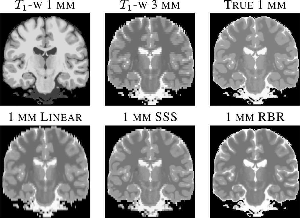
In this experiment, the atlas $\{{𝒜}_1^H,{𝒜}_2^H\}$ consisted of the multiple sclerosis (MS) BrainWeb phantom T₁-w and T₂-w image at 1 mm³ isotropic resolution [21]. The subject ${𝒮}_1^H$ was the normal BrainWeb phantom T₁-w at 1 mm³ isotropic resolution and a resampled low resolution T₂-w image. The regression ensemble was trained on the atlas and then applied to the subject to produce a synthetic high resolution T₂-w image, ${\mathrm{𝒮̂}}_2^H$. We compared to two baseline interpolation methods, nearest neighbor (NN) and trilinear (TL) interpolation, as well as the state-of-the-art self similarity based super-resolution (SSS) [7] by computing the peak signal to noise ratio (PSNR) for each of the four methods. We also varied the through plane slice thicknesses of the input data from 3, 5, and 9 mm with the results shown in Table 1, and example results of the interpolation methods are shown in Fig. 1.

Table 1.

PSNR (dB) results across three input resolutions for each of four methods: nearest neighbor (NN) and trilinear (TL) interpolation, the state-of-the-art SSS [7], and our method—the regression based reconstruction (RBR).

	PSNR
Z Res.	NN	TL	SSS [7]	RBR
3 mm	12.62	12.90	22.71	32.10
5 mm	11.46	11.90	19.69	31.87
9 mm	10.36	10.79	16.94	31.03

Fig. 1.

The top row shows the input data of a HR (1 mm through plane) T₁-w and LR (3 mm through plane) linear interpolated result, as well as the true HR T₂-w image, respectively. The bottom row shows the results of various interpolation approaches. From left to right, trilinear (Linear), self similarity based approach SSS [7], and our regression approach (RBR).

3.2. Super Resolution with Noise on BrainWeb Phantom

In this experiment, the atlas $\{{𝒜}_1^H,{𝒜}_2^H\}$ consisted of the MS BrainWeb phantom T₁-w 1mm³ isotropic resolution, and a corresponding T₂-w image [21]. The atlas T₂-w image was downsampled to 3 mm in plane resolution and upsampled back to 1 mm using linear interpolation, to generate ${𝒜}_2^L$. The subject image ${𝒮}_1^H$ is the normal BrainWeb phantom of a T₁-w and a resampled T₂-w originally at 3mm through plane resolution image with various noise levels. The regression ensemble was trained on the atlas and then applied to the subject to produce a synthetic T₂-w image, ${\mathrm{𝒮̂}}_2^H$. We, again, report PSNR for each of the four interpolation methods (see Table 2).

Table 2.

PSNR (dB) results across five noise levels for each of four methods: nearest neighbor (NN) and trilinear (TL) interpolation, the state-of-the-art SSS [7], and our method—the regression based reconstruction (RBR).

	PSNR
Noise (%)	NN	TL	SSS [7]	RBR
1%	12.62	12.90	19.25	33.93
3%	12.59	12.89	19.64	33.65
5%	12.54	12.87	19.56	33.00
7%	12.47	12.84	19.83	32.20
9%	12.40	12.82	19.56	31.30

3.3. Super Resolution of Real T₂-W Data

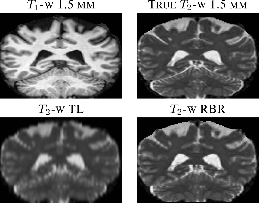
In this experiment we used our regression based reconstruction for the super resolution of T₂-w images from the Kirby data set [22]. We chose 10 subjects from the Kirby data set who went through a scan-rescan protocol, which included a T₁-w MPRAGE and a T₂-w scan, both resampled to 1 × 1 × 1.5 mm³ resolution. We downsampled the T₂-w image to 1 × 1 × 4 mm³ resolution and used it as an input to synthesize the higher resolution image and compared it to the acquired true T₂-w scan. Table 3 shows the average PSNR (and standard deviation) values of the super-resolution T₂-w images with the existing true T₂-w images for three methods over the 10 subjects. Fig. 2 shows our result in conjunction with a trilinear interpolated image and the ground truth T₁-w and T₂-w images.

Table 3.

Mean PSNR (dB) and standard deviation for each of three methods across 10 subjects. The three methods are nearest neighbor (NN) and trilinear (TL) interpolation, and our method—the regression based reconstruction (RBR). The state-of-the-art SSS [7] failed to run on any of the real data. We made several attempts to transform the real data into a usable form for SSS, which did not help.

Mean PSNR (Std. Dev.)
NN	TL	RBR
21.1 (0.77)	22.70 (0.74)	26.40 (0.70)

Fig. 2.

The top row shows the true HR (1 mm through plane) T₁-w and T₂-w images respectively. The second row shows the results of various interpolation approaches, (from left to right) trilinear (TL) and our regression approach (RBR).

3.4. Super Resolution of Real FLAIR Data

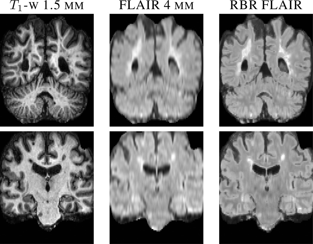
Fluid Attenuated Inversion Recovery (FLAIR) is a pulse sequence used for imaging subjects with MS to best localize their white matter lesions. The lesions appear hyperintense, in FLAIR images, with respect to other tissues and can be easily delineated, for lesion volume quantification. These images are usually acquired at a lower resolution in the through plane direction. The T₁-w images in our data set are at a 1 × 1 × 1.5 mm³ resolution, while the FLAIR images are acquired at 1 × 1 × 4 mm³. We used our algorithm to synthesize high resolution FLAIR images for this data. Fig. 3 shows a visual comparison between an interpolated FLAIR image and our result with the corresponding T₁-w image.

Fig. 3.

The two rows show a super-resolution FLAIR result using our regression approach for two different subjects. From left to right are the original high resolution T₁-w image, the upsampled low resolution input FLAIR and our result (RBR) in the last column.

4. CONCLUSION

We have described a super-resolution scheme for MR images using a model-free, supervised learning technique based on RFs. The presented results are superior to the current state-of-the-art [7]. We also note that in the recent work of Rousseau et al. [9], a super-resolution result on BrainWeb data was reported to have PSNR of 27.62 to 29.53, which we are also superior to. The results of RBR are visually crisper than the other interpolation methods (see Figs. 1, 2, and 3), which could lend itself to localizing structures more accurately. Our method is also computationally efficient and can produce a 256 × 256 × 173-sized image in less than ten seconds. We intend to use this method in automatic segmentation and registration algorithms as a preprocessing step to achieve better results.

REFERENCES

- 1.Greenspan H, Oz G, Kiryati N, Peled S. MRI inter-slice reconstruction using super-resolution. Mag. Reson. Med. 20(5):437–446. doi: 10.1016/s0730-725x(02)00511-8. 2–2. [DOI] [PubMed] [Google Scholar]
- 2.Peeters RR, Kornprobst P, Nikolova M, Sunaert S, Vieville T, Malandain G, Deriche R, Faugeras O, Ng M, Van Hecke P. The use of super-resolution techniques to reduce slice thickness in functional MRI. Int. J. Imaging Syst. Technol. 2004;14(3):131–138. [Google Scholar]
- 3.Hardie RC, Barnard KJ, Bognar JG, Armstrong EE. Joint MAP registration and high-resolution image estimation using a sequence of undersampled images. IEEE Trans. Image Proc. 1997;6(2):1621–1633. doi: 10.1109/83.650116. [DOI] [PubMed] [Google Scholar]
- 4.Tamez-Pena JG, Totterman S, Parker KJ. MRI isotropic resolution reconstruction from two orthogonal scans. Proceedings of SPIE-MI 2001. 2001:87–97. [Google Scholar]
- 5.Bai Y, Han X, Prince JL. Super-resolution Reconstruction of MR Brain Images; Proceedings of the Conference on Information Sciences and Systems (CISS 2004); 2004. [Google Scholar]
- 6.Manjón JV, Coupé P, Buades A, Fonov V, Collins DL, Robles M. Non-local MRI upsampling. Med. Imag. Anal. 2010;14(6):784–792. doi: 10.1016/j.media.2010.05.010. [DOI] [PubMed] [Google Scholar]
- 7.Manjón JV, Coupé P, Buades A, Collins DL, Robles M. MRI Superresolution Using Self-Similarity and Image Priors. International Journal of Biomedical Imaging. 2010;425891:11. doi: 10.1155/2010/425891. [DOI] [PMC free article] [PubMed] [Google Scholar]
- 8.Rousseau F. Proceedings of the European Conference on Computer Vision (ECCV 2008) LNCS; 2008. Brain hallucination; pp. 497–508. [Google Scholar]
- 9.Rousseau F, Studholme C. A supervised patch-based image reconstruction technique: Apllication to brain MRI super-resolution. Proceedings of the International Symposium on Biomedical Imaging (ISBI 2013) 2013:346–349. [Google Scholar]
- 10.Greenspan H. Super-Resolution in Medical Imaging. The Computer Journal. 2009;52(1):43–63. [Google Scholar]
- 11.Baker S, Kanade T. Hallucinating faces; IEEE Intl. Conf. on Automatic Face and Gesture Recog; 2000. pp. 83–88. [Google Scholar]
- 12.Jia K, Gong S. Hallucinating Multiple Occluded Face Images of Different Resolutions. Pattern Recognition Letters. 2006;27:1768–1775. [Google Scholar]
- 13.Konukoglu E, van der Kouwe A, Sabuncu MR, Fischl B. Example-Based Restoration of High- Resolution Magnetic Resonance Image Acquisitions. Medical Image Computing and Computer-Assisted Intervention – MICCAI 2013. 2013;8149:131–138. doi: 10.1007/978-3-642-40811-3_17. [DOI] [PubMed] [Google Scholar]
- 14.Jog A, Roy S, Carass A, Prince JL. Magnetic Resonance Image Synthesis through Patch Regression. Proceedings of the International Symposium on Biomedical Imaging (ISBI 2013) 2013:350–353. doi: 10.1109/ISBI.2013.6556484. [DOI] [PMC free article] [PubMed] [Google Scholar]
- 15.Roy S, Carass A, Prince JL. A Compressed Sensing Approach For MR Tissue Contrast Synthesis; 22nd Conf. on Inf. Proc. in Medical Imaging (IPMI); 2011. pp. 371–383. [DOI] [PMC free article] [PubMed] [Google Scholar]
- 16.Roy S, Carass A, Prince JL. Synthesizing MR Contrast and Resolution through a Patch Matching Technique. Proceedings of SPIE-MI 2010. 2010 doi: 10.1117/12.844575. [DOI] [PMC free article] [PubMed] [Google Scholar]
- 17.Roy S, Jog A, Carass A, Prince JL. Atlas Based Intensity Transformation of Brain MR Images. Multimodal Brain Image Analysis. 2013;8159:51–62. [Google Scholar]
- 18.Breiman L, Friedman JH, Olshen RA, Stone CJ. Classification and Regression Trees. Statistics/Probability Series. Wadsworth Publishing Company, U.S.A.; 1984. [Google Scholar]
- 19.Breiman L. Bagging Predictors. Machine Learning. 1996;24(2):123–140. [Google Scholar]
- 20.Kwan RKS, Evans AC, Pike GB. MRI simulation-based evaluation of image-processing and classification methods. IEEE Trans. Med. Imag. 1999;18(11):1085–1097. doi: 10.1109/42.816072. [DOI] [PubMed] [Google Scholar]
- 21.Landman BA, et al. Multi-parametric neuroimaging reproducibility: A 3-T resource study. NeuroImage. 2011;54(4):2854–2866. doi: 10.1016/j.neuroimage.2010.11.047. [DOI] [PMC free article] [PubMed] [Google Scholar]