TRACTOGRAPHY DENSITY AND NETWORK MEASURES IN ALZHEIMER’S DISEASE

Abstract

Brain connectivity declines in Alzheimer’s disease (AD), both functionally and structurally. Connectivity maps and networks derived from diffusion-based tractography offer new ways to track disease progression and to understand how AD affects the brain. Here we set out to identify (1) which fiber network measures show greatest differences between AD patients and controls, and (2) how these effects depend on the density of fibers extracted by the tractography algorithm. We computed brain networks from diffusion-weighted images (DWI) of the brain, in 110 subjects (28 normal elderly, 56 with early and 11 with late mild cognitive impairment, and 15 with AD). We derived connectivity matrices and network topology measures, for each subject, from whole-brain tractography and cortical parcellations. We used an ODF lookup table to speed up fiber extraction, and to exploit the full information in the orientation distribution function (ODF). This made it feasible to compute high density connectivity maps. We used accelerated tractography to compute a large number of fibers to understand what effect fiber density has on network measures and in distinguishing different disease groups in our data. We focused on global efficiency, transitivity, path length, mean degree, density, modularity, small world, and assortativity measures computed from weighted and binary undirected connectivity matrices. Of all these measures, the mean nodal degree best distinguished diagnostic groups. High-density fiber matrices were most helpful for picking up the more subtle clinical differences, e.g. between mild cognitively impaired (MCI) and normals, or for distinguishing subtypes of MCI (early versus late). Care is needed in clinical analyses of brain connectivity, as the density of extracted fibers may affect how well a network measure can pick up differences between patients and controls.

1. INTRODUCTION

Alzheimer’s disease (AD) is the most common form of dementia worldwide, and to date has no known cure. To evaluate new treatments, image-based measures of disease progression are urgently sought, and diffusion imaging has recently been added to several large-scale studies of AD in the hope of capturing breakdown in brain integrity and connectivity not detectable with standard anatomical MRI. The connectivity of the white matter progressively declines in AD [1, 2], but it is not yet known which connectivity measures best distinguish patients from controls, and how robust these measures are to specific aspects of the methods used, such as the density of extracted fibers. Here we studied brain networks in people with AD, in those at heightened risk for AD (with an intermediate stage of the disease known as mild cognitive impairment (MCI)), and in healthy elderly subjects using structural magnetic resonance imaging (MRI) and diffusion MRI. We aimed to identify (1) which network measures best distinguish AD from healthy controls, and (2) the influence of tractography density on these measures. Our data is from the Alzheimer’s Disease Neuroimaging Initiative (ADNI) [3], an endeavor to find and evaluate biomarkers that capture disease progression or help predict risk for AD. We studied the imaging data from 110 subjects in total - 28 controls (C), 11 with late-stage mild cognitive impairment (L-MCI), 56 early MCI (eMCI), and 15 AD.

We used global probabilistic tractography to capture the structure of the white matter. The method leverages all the diffusion direction information parameterized by the orientation diffusion function (ODF). We accelerated the method by using a lookup table of diffusion values from the ODF. Cook et al. [4] used a lookup table in diffusion data, but they focused on the probability density function while our approach is specifically designed to speed up tractography. Our optimized tractography algorithm allows us to quickly compute thousands of fibers per subject and study how this density affects our network connectivity measures.

We describe the specifics of our subject data and how we preprocess it for connectivity analysis. Our optimization of the global probabilistic tractography is detailed including a rapid method to access the pre-computed information in the look-up table. We then detail how we compute connectivity matrices and network measures, which are the features used to compare the different disease categories. The details of these results are analyzed and discussed to understand the interplay of fiber density, network measures, and disease.

2. METHODS

2.1. Data

Our data consisted of 110 subjects from ADNI-2, a continuation of the ADNI project in which diffusion imaging was added to the standard MRI protocol. The dataset as of 11/01/12 included 28 cognitively normal controls (C), 56 early- and 11 late-stage MCI subjects (eMCI, LMCI), and 15 with Alzheimer’s disease (AD).

The subjects were scanned on 3-Tesla GE Medical Systems scanners, which collected both T1-weighted 3D anatomical spoiled gradient echo (SPGR) sequences (256 × 256 matrix; voxel size = 1.2 × 1.0 × 1.0 mm³; TI=400 ms; TR = 6.98 ms; TE = 2.85 ms; flip angle = 11°), and diffusion weighted images (DWI; 256 × 256 matrix; voxel size: 2.7 × 2.7 × 2.7 mm³; scan time = 9 min). The DWI images were composed of 41 diffusion images with b = 1000 s/mm² and 5 T2-weighted b₀ images. This protocol was chosen after an effort to study trade-offs between spatial and angular resolution in a tolerable scan time [5].

2.1.1. Image Preprocessing

We processed the T1-weighted images to parcellate them into 68 cortical regions. We first automatically removed extra-cerebral tissues from the anatomical images using ROBEX [6], a method that learned from manual T1-weighted segmentations of hundreds of healthy young adults. These skull-stripped brains were inhomogeneity corrected using the MNI N3 tool [7] and aligned to the Colin27 template [8] with FSL Flirt [9]. The resulting images were segmented into 34 cortical regions (in each hemisphere) using FreeSurfer [10]. These segmentations were then dilated with an isotropic box kernel of 5 × 5 × 5 voxels to make sure they intersected with the white matter for subsequent connectivity analysis.

We corrected head motion and eddy current distortion in each subject by aligning the DWI images to the average b₀ image with FSL’s eddy correct tool. The brain extraction tool (BET) [11] was then used to skull-strip the brains because we did not have manual segmentations for ROBEX. We EPI corrected these images with an elastic mutual information registration algorithm [12] that aligned the DWI images to the T1 scans. More detail on these preprocessing steps is given in [13]. The registration here should not effect the subsequent connectivity analysis greatly because the labels have been dilated to make sure they intersect with the white matter fibers.

2.2. Tractography

We employed a global probabilistic tractography method based on the Hough transform [14]. The method takes advantage of all the diffusion information provided at each voxel, parametrized by the orientation distribution function (ODF). We note that although the ADNI DTI protocol is not a high-angular resolution imaging protocol, the use of an explicit ODF model rather than a single-tensor model makes best use of the available angular resolution, which is inherently limited as many patients cannot tolerate a long scan.

The Hough method generates curves in the fiber space and scores them based on fractional anisotropy (FA) and the ODF at each point along the curve. The scoring function is

$$\int \left(\log \right[\mathrm{FA}\left(\overrightarrow{x}\right(s\left)\right){\mathrm{ODF}}_{\overrightarrow{x}\left(s\right)}\left(\widehat{t}\right(s\left)\right)]+\lambda \mathit{ds}),$$ (1)

where s is the arc length along the curve, $\widehat{t}$ the unit tangent vector, $\overrightarrow{x}$ denotes the coordinates along the curve, and λ is a prior on the length of the fibers (it is tuned so that curves oriented towards the cortex will be long enough to reach the gray matter). FA was computed from the single-tensor model of diffusion [15]. The method then computed the ODF at each voxel from the diffusion data with a normalized and dimensionless estimator derived from Q-ball imaging (QBI) [16]. This formulation includes the Jacobian factor r² in the constant solid angle (CSA) ODF, defined as

$$\frac{1}{4\pi }+\frac{1}{16{\pi }^2}\text{FRT}\left\{{\nabla }_b^2\ln \left(-\ln \frac{S\left(\widehat{u}\right)}{S_0}\right)\right\},$$ (2)

where $S\left(\widehat{u}\right)$ is the diffusion signal in unit direction $\widehat{u}$ , S₀ is the baseline image, FRT is the Funk-Radon transform, and ${\nabla }_b^2$ is the Laplace-Beltrami operator. This model is more accurate and outperforms the previous QBI definition [17], giving greater resolution for detecting multiple fiber orientations [16, 18] and additional information for the scoring function.

The Hough transform tractography method searches through a set of seed locations for the highest scoring curves. These 3D curves are parameterized by their arc length with s = 0 centered at a seed point. The curve’s unit tangent vector, $\widehat{t}$, is described by standard polar coordinates, θ(s) and ϕ(s), which are each approximated by an N order polynomial. In addition, there are parameters L₋ and L₊ that decide the partial length along either side of the seed point. These parameters are set to include fibers that can span the white matter in the image space. The coordinates are found by integrating the tangent vector as

$$\overrightarrow{x}\left(s\right)={\overrightarrow{x}}_0+{\int }_0^s\widehat{t}\left(s^{\prime }\right){\mathit{ds}}^{\prime },$$ (3)

where s ∈ [−L₋, L₊], and ${\overrightarrow{x}}_0$ is the seed location. This characterization means that the method will represent each curve using 2N+4 parameters and uses the voting process provided by the Hough transform to select the best fitting curve for a seed. If we restrict our search space to polynomials of order N = 3 and the maximum length to be longest expected fiber length in an image, the complete search at each seed point can result in millions of curves and upwards of one minute of computation time per seed, taking weeks to complete tractography on a single subject.

2.2.1. Optimizations

We optimized the Hough transform tractography method with an ODF lookup table and a random search through the curve parameter space.

The Hough tractography method spends most of its computational time finding diffusion values at tangent directions along possible curves by evaluating the ODF. ODFs are represented as a spherical harmonic series, and this consumes a great deal of time after millions of evaluations. We remedy this issue with a lookup table that stores diffusion data in a set of random directions and is pre-computed before the Hough method evaluates the scores of the sampled curves. This saves time because the method does not have to evaluate the spherical harmonic series every time a curve point is evaluated and has immediate access to the diffusion information. We created the table by selecting n random directions, evaluating the ODFs at each voxel in our image at those directions, and then storing the resulting diffusion values in an array.

In addition, we created a direction lookup table that stores the index of the closest direction for an arbitrary θ and ϕ. This table allows us the query the ODF lookup table without comparing a requested direction to our n random direction each time we need to evaluate the ODF. We created the table by first selecting the range 0 to 2π for both θ and ϕ and sample this range at m points, giving m² possible pairs of (θ, ϕ). For these pairs we compute the closest direction, α, from our set of n random directions that satisfies

$$\underset{\alpha }{\mathrm{argmax}}\left(\mid \frac{\overrightarrow{\alpha }\cdot \overrightarrow{\beta }}{\Vert \overrightarrow{\alpha }\Vert \Vert \overrightarrow{\beta }\Vert }\mid \right),$$ (4)

where β is a possible (θ, ϕ) combination. This distance is the absolute value of the cosine of the angle between the two directions α and β. The absolute value is necessary because of the symmetry found in the ODF. Fig. 1 shows an example table for n = 1000 random directions and m = 1000 points between 0 to 2π. Each color represents the index of the closest random direction for each (θ, ϕ) pair.

Fig. 1.

The directions lookup table affords immediate access to precomputed ODF information without having to compute the closest angle for a direction query. The colors represent the closest precomputed ODF direction for each θ and ϕ combination (each color represents the index or label for the closest pre-computed direction). This example shows n = 1000 random directions sampled on the sphere, with θ and ϕ ranging from 0 to 2Π with m = 1000 intervals. This range is chosen to coincide with the query range from the Hough transform method.

We also cut down the computation time by randomly selecting a subset of the curve parameters to search. In our experiments we found that a search that covered only 10% of the parameter space would give a very close approximation to the exhaustive results. Together the random search and lookup table reduced the computation time for a single seed to less than one second and for an entire image to a matter of hours.

In our experiments, this arrangement of relying on a large precomputed database accessed by many smaller threads is well suited to the MapReduce model [19] to distribute computations to grid resources. In particular, our lookup table was designed to be accessed with low latency using the distributed file system provided by Apache Hadoop, an open-source implementation of MapReduce.

We used the optimized Hough transform tractography method to compute 50, 000 fibers in each of our subjects. Fig. 2 compares 50, 000 and 50, 000 fibers in the same subject.

Fig. 2.

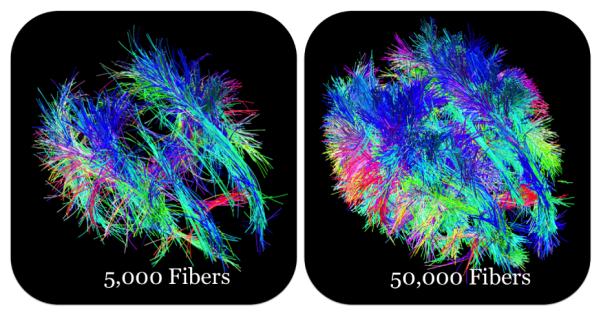
Fibers from the optimized Hough transform tractography method. We contrast two different densities of fibers.

2.3. Connectivity

From the tractography results, we created connectivity matrices that measure the number of detected fibers that connect cortical regions to each other. To create a subject’s matrix, we went through each of the fibers and compared it to the dilated cortical labels. The labels that intersected the fiber were logged into the connectivity matrix. This results in a 68 × 68 connectivity matrix for each subject as shown in Fig. 3. The figure shows the intra-hemispheric connections in the top-left and bottom-right squares and the inter-hemispheric connections in the bottom-left and top-right areas. The colors signify how many fibers connect the two regions. We refer to this as the fiber density, while noting that the actual density of axonal fibers can only be determined histologically. Also the relation of our measure to the actual fiber density is complex as it depends on the seeding of the curves and the size of the ROIs on the cortex (for this reason, some other definitions normalize the fiber counts based on the areas of the cortical ROIs they interconnect).

Fig. 3.

A sample connectivity matrix from our subject data showing connections in the left and right hemispheres. The colors signify how many fibers compose each connection.

We computed ten connectivity matrices for each subject. Each of these differed in the number of fibers used to create the matrix -ranging from 5,000 to 50,000, in increments of 5,000.

2.4. Connectivity Measures

We interpreted our connectivity matrices with eight network measures described in [20], computed with the Brain Connectivity Tool-box. We chose global efficiency, transitivity, path length, mean degree, density, modularity, small world, and assortativity. We computed global efficiency, transitivity, path length, density, modularity, and small world in both weighted and binary undirected networks. Ten different thresholds were applied to each connectivity matrix, to preserved a fraction of the weights ranging from .1 to 1 by intervals of .1. We note that such a thresholding operation is common in network analysis (cf. work on “k-cores” [21] or Rips filtrations [22]), to retain subnetworks that contain the highest density of connections, and eliminate low density connections, to better understand overall network organization.

2.5. Experiments

For each subject, we computed ten different connectivity matrices, for these matrices we computed a total of fourteen different network measures at ten different weight preservation thresholds. The resulting measures were then used for two-sample t-tests comparing controls vs. eMCI, controls vs. L-MCI, controls vs. AD, and eMCI vs. L-MCI across fiber count and threshold amount. This setup was intended to show how fiber density influences connectivity network measures.

3. RESULTS

Fig. 4 shows p-values from the t-tests comparing different disease states in our data, as a function of the number of fibers used to create the connectivity matrices. We hypothesized that the group differences would show greater effect sizes (smaller P-values) as fiber density increased. The measures identified in the legend are global efficiency (GT), transitivity (T), path length (PL), mean degree (MD), density (D), modularity (M), small world (SM), and assortativity (A), with (b) and (w) signifying binary and weighted undirected connectivity matrices respectively. In the control vs. AD graph we retained 90% (based on searching through thresholds ranging from .1 to 1 at intervals of .1) of the weights for the connectivity matrices used to generate the figure and measures wSW, bSW, bPL, bM, bGE, bD, wPL, wM, wGE easily passed the p = .05 threshold. bT was able to pass the threshold when 45, 000 or greater fibers were used to create the connectivity matrix. Assortativity and Transitivity had a difficult time distinguishing the two classes, though binary transitivity passed the 0.05 threshold at 45, 000 fibers.

Fig. 4.

p-values from two-sample t-tests comparing controls vs. AD subjects, controls vs. eMCI, and eMCI vs. L-MCI using twelve network measures across different numbers of fibers used to create the connectivity matrix. The best network measure for distinguishing subjects in the eMCI tests was the mean nodal degree (MD). The differences were strong enough to survive multiple comparisons correction for the 12 network measures assessed, and for the search with respect to the number of fibers, and with respect to the network sparsity threshold.

In the control vs. eMCI part of Fig. 4 we shows that bT passed the p = .05 threshold at 15, 000 fibers and bM passed it at 30, 000 and 45, 000 while MD becomes very highly significant with 20, 000 fibers or more. A threshold of 20% (this was the best performing threshold based on the ten we searched through) was applied to the connectivity matrix weights. Weighted modularity and path length were the worst performers in this test.

We also show results from eMCI versus L-MCI in Fig. 4. In this case, we present results where a 20% threshold is applied. bPL and bM became significant at 50,000 fibers. Again, MD becames highly significant at 20, 000 fibers or greater. Clearly, there is some minimal acceptable density to create an accurate network, but the addition of more samples also reduces noise, further boosting effect sizes. Weighted modularity and binary global efficiency were the worst performers and stable across the fiber counts.

Table 1 shows the most significant measure for each test along with its p-value, fiber count, and the optimal threshold used to create the connectivity matrices. It may be that the AD effect is so strong that it can be found no matter what the threshold is, but the MCI effect may be more subtle requiring a judicious choice of settings, in our case a 20% threshold. Mean density performed the best in three of the categories and is the same for weighted and binary connectivity matrices.

Table 1.

Most significant results, i.e. highest effect sizes, in our network measure comparison between disease states. C represents controls and % shows the percentage of weights retained in the connectivity matrices. The mean degree of the network was highly effective at distinguishing different phases of the disease.

Test	Measure	p-value	Fibers	%
C vs. AD	wSW	4:28 × 10−6	50k	90
C vs. eMCI	MD	2:92 × 10−12	40k	20
C vs. L-MCI	MD	1:17 × 10−3	50k	20
eMCI vs. L-MCI	MD	2:50 × 10−8	50k	20

4. DISCUSSION

Our results showed that in some cases a larger number of fibers provided more significant results. Weighted small world in controls vs. AD and mean degree on the MCI comparisons seemed very sensitive to fiber density. The variability in p-values at the 50,000 fiber count may be the result of a decrease in the number of subjects for the test. In a few of the subjects there were less than 50,000 seed points with only 86 of the 110 represented at that fiber count level.

The advantage of more fibers could be higher for catching subtle differences in controls vs. MCI stages or differences between MCI stages. In the case of controls vs. AD, the network may be so different that the network is not influenced by fiber counts as much.

Mean degree stood out among the network measures in differentiating the disease groups; further studies may be useful evaluating other degree-related measures, including subnetworks derived by filtering the networks by nodal degree (such as K-cores).

Our optimization of the Hough transform tractography method made the large fiber counts feasible in a reasonable amount of computation time. Future work will focus on more formally bounding the errors in the lookup table and random search compared to the original implementation. In addition, it would be helpful to derived the time and space complexity for the method and a careful study of them for different datasets.